Chandra X-ray Observation of the Orion Nebula Cluster. I Detection, Identification and Determination of X-ray Luminosities

Abstract

In this first of two companion papers on the Orion Nebula Cluster (ONC), we present our analysis of a 63 Ksec Chandra HRC-I observation that yielded 742 X-ray detections within the $30^{\prime}\times 30^{\prime}$ field of view. To facilitate our interpretation of the X-ray image, here we collect a multi-wavelength catalog of nearly 2900 known objects in the region by combining 17 different catalogs from the recent literature. We define two reference groups: an infrared sample, containing all objects detected in the $K$ band, and an optical sample comprising low extinction, well characterized ONC members. We show for both samples that field object contamination is generally low.

Our X-ray sources are primarily low mass ONC members. The detection rate for optical sample stars increases monotonically with stellar mass from zero at the brown dwarf limit to $\sim 100\%$ for the most massive stars but shows a pronounced dip between 2 and 10 solar masses.

We determine $L_{X}$ and $L_{X}/L_{bol}$ for all stars in our optical sample and utilize this information in our companion paper to study correlations between X-ray activity and other stellar parameters.

1 Introduction

The Orion region is one of the most frequently observed areas of the sky. It comprises several molecular clouds and stellar associations, among which the Orion Nebula Cluster (ONC - also referred to as the Trapezium region), is of particular interest. With an age of about 1 million years, more than two thousand young stellar objects with masses between 0.08 and 50$M_{\odot}$, an estimated central density of $\sim 2\times 10^{4}$ stars per cubic parsec, and at a distance of $\sim 470$pc, it is the largest and densest concentration of young pre-main sequence (PMS) stars in our region of the Galaxy. Only part of the ONC members – those lying on the near side of the Orion Molecular Cloud from which the cluster is forming – are optically visible; more than half are so deeply embedded in the cloud that they are observable only at infrared (IR) or X-ray wavelengths where the cloud becomes more transparent. For more complete descriptions of the ONC structure, dynamics, and stellar content, see Hillenbrand (1997); Hillenbrand & Hartmann (1998); Hillenbrand & Carpenter (2000); Carpenter (2000); Luhman et al. (2000); O’Dell (2001), and references therein. Among others, Hillenbrand and collaborators (Hillenbrand, 1997; Hillenbrand et al., 1998; Hillenbrand & Carpenter, 2000) have extensively studied both the optically visible and the embedded ONC stellar content. Several studies (Stassun et al., 1999; Herbst et al., 2000, 2001; Rebull, 2001) have measured rotational periods via photometric modulation of stellar spots. Spectacular HST images (see e.g., Bally et al., 2000) have allowed the direct observation of many circumstellar disks and proplyds (photoionization structures due to the evaporation of disks) that seem to surround a large fraction of the PMS stars in the vicinity of the central bright star $\theta^{1}$ Orionis C.

The ONC was first detected in the X-rays by the Uhuru satellite (Giacconi et al., 1972). Following imaging observations performed with the Einstein and ROSAT observatories (Ku & Chanan, 1979; Gagné et al., 1995) indicated that: a) ONC members are powerful X-ray emitters, with typical $L_{X}/L_{bol}$ close to the saturation value, $10^{-3}$, observed for fast rotators on the main sequence; b) no relation seems to hold between X-ray activity and stellar rotation; c) stars with circumstellar accretion disks may have lower levels of X-ray activity. These works were however hindered by the lack, at that time, of complete optical information on the ONC population and by the low sensitivity and spatial resolution of the X-ray instrumentation, especially important to resolve the dense central region and to unambiguously identify X-ray sources with optical counterparts. Both of these limitations have been recently lifted: Chandra observations (Schulz et al., 2001; Garmire et al., 2000) have revealed about 1000 X-ray point sources, for the most part associated with low mass stars down to the substellar mass limit.

In this work we describe the analysis of a Chandra High Resolution Camera (HRC, Murray et al., 2000) observation of the ONC and correlate our data with relevant data from the literature. In a companion work (Flaccomio et al. 2002; hereafter Paper II), we investigate statistical correlations between X-ray activity and other stellar characteristics (such as rotational period, mass, age and disk accretion indicators) and search for insights into the physical mechanisms that drive activity in PMS stars. An investigation of the X-ray variability characteristics of ONC members based on these data is in preparation.

The structure of this paper is as follows: we first introduce our Chandra observation and discuss its reduction and X-ray source detection (§2). We then describe the preparation of an extensive catalog of known X-ray/optical/IR/radio objects in the region of our HRC observation, collecting from the literature useful observable properties and defining two reference object samples (§3). In the same section we also report the results of our observation in the BN/KL region. In §4 we concentrate on the optical/IR properties of our X-ray sources, and in §5 and a supporting Appendix, we determine the X-ray activity indicators $L_{X}$ and $L_{X}/L_{bol}$, along with their uncertainties. Our findings are summarized in §6, setting the stage for Paper II.

2 Observation and Data Reduction

The HRC on board the Chandra X-ray Observatory (Weisskopf et al., 2002) observed the ONC for 63.2 ksec on 2000 February 4. The pointing ($R.A._{2000}=5^{h}:35^{m}:17^{s}$, $DEC._{2000}=-5^{\circ}:23^{\prime}:16^{\prime\prime}$) was chosen to place the Trapezium region and the bright O star $\theta^{1}$ Orionis C in the center of the field of view (FOV). A good fraction of the ONC region was included in the $30^{\prime}\times 30^{\prime}$ HRC FOV.

Our Chandra observations offer these significant improvements over previous Einstein and ROSAT observations: unprecedented spatial resolution ($\sim 0.5^{\prime\prime}$ in the field center), important in such a crowded field (see §3.2); sensitivity $\sim 20$ times deeper than previous X-ray data (see §5); and continuous temporal coverage for variability studies.

2.1 Data Filtering

Our HRC analysis begins by filtering the event list to lower background levels and increase the source signal-to-noise ratio (SNR). We considered filtering out particular time intervals and/or ranges of pulse height amplitude ($PHA$) dominated by instrumental and spacecraft environment effects. We examined light curves of the entire observation but found that our particular data set did not suffer from variable solar activity contamination commonly reported for Chandra data. Hence no time filtering was applied. On the other hand, $PHA$ distributions of all events do show a sharp instrumental peak for $PHA$ values $\lesssim 35$, and as in our previous HRC analyses (Harnden et al., 2001), we excluded this peak by eliminating events with $PHA<35$. Given the $PHA$ response of the HRC to X-rays and stellar spectra (cf. §5.1), these counts are almost exclusively background: total events were reduced by about $15\%$ (from $\sim 2.1$ to $\sim 1.8\times 10^{6}$), while source counts declined only $\sim 1\%$.

Figure 1 shows the filtered HRC image, smoothed for presentation purposes with the csmooth task in the Chandra Interactive Analysis of Observations (CIAO) package, available at $\rm http://asc.harvard.edu/ciao/$.

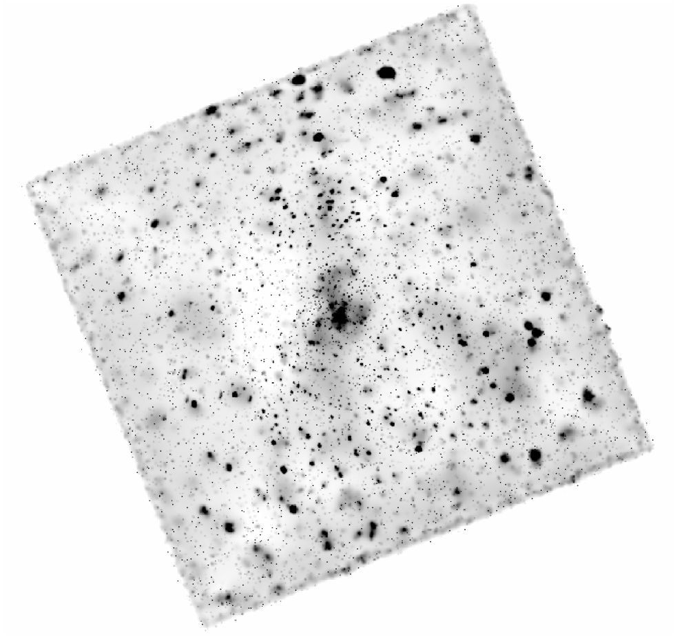
Figure 1: HRC-I image of the ONC processed with csmooth. Linear gray scale indicates photon arrival rate vs. position on the detector. In this low-resolution presentation black indicates scale saturation due to intense point-like sources (or unresolved groups of sources). Note that the PSF increases significantly toward image edges.

2.2 Source detection

We have analyzed the filtered event list with the Palermo Wavelet Transform detection code, pwdetect (Damiani et al., 1997, 2002). In synthesis, pwdetect analyzes an image at a variety of spatial scales, allowing detection of both point-like and moderately extended sources. The most important parameter required by the code is the detection threshold which determines, along with the image background level, the number of expected spurious detections. The relationship between detection threshold and expected number of spurious sources was determined by running the pwdetect code on 400 simulated background images with roughly the same number of photons as in the background of our observation ($\sim 1.46\times 10^{6}$, once the source contribution is removed).

We choose to accept detections with $SNR>4.74$, corresponding to 10 expected spurious detections throughout the FOV. We accept 10 spurious sources, instead of the more customary one, for three reasons: i) 10 is still a small fraction of the total number of detected sources, ii) by lowering the threshold from $5.25\sigma$ (corresponding to 1 spurious source) to 4.74, we gain $\sim 100$ good detections (after a “hand filtering” of the detection list – see below), of which only 9 are expected to be spurious, and iii) as shown in §3.2, Chandra’s superb spatial resolution ensures that the $\sim 10$ spurious sources are extremely unlikely to be identified with other wavelength counterparts.

Visual inspection of the initial lists of $\sim 830$ detections produced by pwdetect showed that although the vast majority of detections appear real and most of the obvious sources in the image are detected, two “glitches” of the detection algorithm produce undesired effects. First, about 90 sources are detected in the vicinity of very bright stars, notably on the wings of the point spread function (PSF) of the central source ($\theta$ ¹Ori C). These are most likely spurious detections due to large intensity fluctuations on the wings of bright sources. In such regions the code is unable to estimate correctly the highly spatially variable background level. Second, in a few cases ($\sim 20$) a pair of sources clearly visible and distinguishable by eye in the X-ray image is detected as both a point source corresponding to one of the two and an extended source encompassing the pair. We dealt with the first problem (to be addressed in a future version of pwdetect) by visually examining the list of detections and excluding the spurious sources in question. Specifically, we deleted all sources lying closer than 6.8” to $\theta^{1}$ Orionis C, thereby also losing any real sources occurring in that area. The second problem occurs because the extended detection has a higher SNR than the point-like detection. For such cases, we eliminated this problem by running a special version of pwdetect that limits its search to point-like sources.

pwdetect estimates positions and count rates of detected sources in the assumption that the PSF is Gaussian. Since the actual HRC PSF is not Gaussian, we investigated the effect of this simplifying assumption on our estimates. We computed the wavelet transform of calibration PSFs (in the Chandra Calibration Database; see asc.harvard.edu/caldb) at several detector positions and for a representative energy of $\sim 1.5$ keV. In order to better match the actual shape of bright sources in our HRC image, these calibration PSFs were first convolved with a bi-dimensional Gaussian with $\sigma=0.3^{\prime\prime}$, possibly reflecting the effect of imperfect aspect reconstruction affecting the real source PSF. Corrections respect to the Gaussian PSF approximation were parametrized as a function of off-axis angle and, for count rates, range from 16% at the field center to 0% at $\gtrsim 10^{\prime}$ off-axis. Having verified that this result agrees well with the (background-subtracted) extracted counts of bright isolated sources in the limit of large extraction radii, we applied the correction to our source count rates. Positional errors (up to $0.9^{\prime\prime}$ for off-axis angles of $\sim 14^{\prime}$) are instead always much smaller respect to random uncertainties and were therefore neglected.

The final lists of detections, comprising 742 X-ray sources, is presented in Table 1 where we give sky position and its statistical uncertainty, detection SNR, number of source counts and uncertainty, and effective exposure time at the source positions. This latter quantity, describing the spatially varying sensitivity of the HRC plus Chandra mirror system, is derived from an exposure map calculated with CIAO for an incident energy of 2.0 keV, i.e., the approximate temperature of our sources (see §5.1). This choice of temperature is not critical for our purposes, however, because the normalized effective area at any given point on the detector depends only marginally on energy: for $0.5<kT<3.5$, the values of effective exposure times at any given location on the detector vary at most at the $\sim$4% level.

Table 1: X-ray sources detected in the Orion Nebula Cluster

$N_{X}$	$Ra(2000)$	$Dec(2000)$	$\delta_{Ra,Dec}$	$SNR$	$Counts$	$\delta_{cnts}$	$Exp.T.$
	[$~{}h$ $~{}m$ $~{}s$]	[∘  ′  ′′]	[′′]				[ks]
(1)	(2)	(3)	(4)	(5)	(6)	(7)	(8)
1	5 34 14.46	-5 28 16.62	3.38	36.27	1277.75	67.97	49.06
2	5 34 18.23	-5 33 28.53	6.91	6.65	167.54	41.78	47.64
3	5 34 20.70	-5 30 46.81	5.90	9.21	259.90	46.23	49.44
4	5 34 20.74	-5 23 25.85	8.03	4.76	111.66	33.69	51.22
5	5 34 24.96	-5 22 6.32	3.17	42.89	1095.36	46.16	52.24
6	5 34 27.23	-5 24 22.23	2.02	63.91	1866.58	64.05	52.90
7	5 34 27.69	-5 31 55.39	3.17	42.05	1536.32	72.59	50.23
8	5 34 28.53	-5 24 58.95	2.20	50.53	1225.93	49.62	53.21
9	5 34 29.09	-5 14 32.51	4.46	15.73	434.32	225.67	49.69
10	5 34 29.30	-5 23 56.09	2.30	45.86	1024.30	45.09	53.52

Note. — The 742 entries of the full table are available in electronic form at: http://www.astropa.unipa.it/$\sim$ettoref/PaperI_tables.html

In addition to measuring count rates for detected X-ray sources, we also used pwdetect to compute upper limits to the photon flux of all non-detected objects in the catalog described in the next section. This calculation was performed consistently using the same SNR threshold as for detections and applying the correction, described above, due to the non-Gaussian PSF.

3 The general catalog of known objects

We assembled an extensive catalog of known X-ray/Optical/IR and radio objects that fell within the HRC FOV. In addition to our list of HRC sources and the Chandra source lists of Garmire et al. (2000) and Schulz et al. (2001), we considered 14 catalogs from recent publications, producing a database of nearly 2900 distinct objects reported in at least one of the studies considered. A full list of references is given in the first column of Table 2 along with a concise classification of the work (col. 2) and the referenced table number(s) from the original work (col. 3).

3.1 Catalogs cross-identifications

Cross identifications were based on positional coincidence. First of all we registered the coordinates of each catalog to a standard reference list (that of Jones & Walker, 1988) using the mean relative displacement of well identified objects. In the case of the Garmire et al. (2000) list of X-ray sources, we also had to apply a rotation of 0.21^∘ around the HRC field center in order to bring the coordinates into agreement with those of the other lists. We then performed the final identifications using the following tolerances: a) For our list of HRC X-ray sources, the positional uncertainties computed by pwdetect as a function of source statistics and off-axis angle. These range from $0.036^{\prime\prime}$ for the bright central source ($\theta^{1}$ Ori C) to $\sim 8^{\prime\prime}$ for weak sources close to the detector border. b) For the Chandra sources of Garmire et al. (2000), uncertainties were assumed to follow the same off-axis trend as measured in our data. We performed a fourth order polynomial fit of HRC position errors vs. off-axis angle and then conservatively used twice these values for the Garmire et al. (2000) source off-axis angles (to allow for additional counting statistics effects). c) For all other catalogs, we used $\sim 2.5$ times the mean dispersion of the registered position offsets with respect to the reference list (Jones & Walker, 1988). In all cases, this identification radius was $\lesssim 1.0^{\prime\prime}$.

We then examined the resulting list of identifications by eye and modified some identifications according to more subjective criteria. For example, 9 X-ray sources detected at large off-axis ($\gtrsim 8^{\prime}$), and therefore with relatively large PSFs, were associated with one or two optical objects that fell outside the error circle. In these cases these optical objects lay well within the PSF and thus potentially contributed the detected photons. In some of these cases the source centroid lay between two objects unresolved (by pwdetect) so neither was within the formal error circle. In all such cases we added the missing identifications manually.

Table 2: List of catalogs in the ONC area.

Reference	Type of study	Table	Num	$R_{95}$	$N_{R}$	$N_{HRC}$	Data
This work	X-ray (HRC-I)	1	742	2.2	553	-	HRC-I Cnt. rate
Schulz et al. (2001)	X-ray (ACIS-S)	1	111	0.4	63	92	ACIS-S Cnt. rate
Garmire et al. (2000)	X-ray (ACIS-I)	1	971	1.4	559	579	-
Bally et al. (2000)	Optical (HST)	1,2	48	0.5	17	14	-
Hillenbrand (1997)	Optical Phot./Spec.	1,3	1516	0.4	1055	627	$V^{1}I^{2}$ $A_{V}^{2}$ $T_{eff}$ $L_{bol}$
Hillenbrand et al. (1998)	IR Photometry	1	1516	-	-	627	$J^{2}H^{3}K^{2}L^{2}$ $EW_{CaII}$ $\Delta_{I-K}$
Hillenbrand & Carpenter (2000)	IR Photometry	1	776	0.4	242	282	$H^{1}K^{1}$
Lucas & Roche (2000)	IR Photometry	1	557	0.7	102	116	$I^{1}J^{1}H^{2}$
Lucas et al. (2001)	IR Spectroscopy	1,3	23	-		2	$A_{V}^{1}$ $Mass$
Lada et al. (2000)	IR Phot. Protostars	1	78	0.5	11	26	$L^{1}$
2Mass	IR Photometry	-	1596	0.6	728	416	$J^{4}H^{5}K^{4}$
Carpenter et al. (2001)	IR Phot. / Variability	4,7	555	0.5	379	241	$J^{3}H^{4}K^{3}$ $P_{rot}^{4}$
Stassun et al. (1999)	$P_{rot}$	1	124	0.5	115	84	$P_{rot}^{3}$
Herbst et al. (2000)	$P_{rot}$	2	132	-		109	$P_{rot}^{2}$
Herbst et al. (2001)	$P_{rot}$	-	296	-		168	$P_{rot}^{1}$
Jones & Walker (1988)	Proper Motion	3	1034	-		519	$P_{memb}$
Felli et al. (1993)	Radio	1,5	49	0.9	18	25	-
Reid (private comm.)	Radio	-	100	0.4	32	43	-

The end result is a table (not shown) with 15 columns, one for each catalog, and 2887 rows, each row representing the cross-identifications of a single object. Table 2 gives, for each catalog, the number of objects in the HRC FOV (col. 4). Column 5 gives a measure of the relative uncertainty in the catalog coordinates, $R_{95}$, representing the 95% quantile of the object’s offsets from the stars of the reference catalog (Jones & Walker, 1988). Column 6 reports the number of objects used in the latter calculation. With typical values of $R_{95}\sim 0.5^{\prime\prime}$, the number of uncertain or ambiguous identifications is indeed small. The number of objects in each catalog identified with an HRC X-ray source is given in column 7. In the next section we discuss in detail the important issue of the reliability and uniqueness of these HRC source identifications.

3.2 X-ray source identification

The outstanding sharpness of the Chandra PSF, especially in the field center, makes it possible for the first time to identify detected X-ray sources as easily as can be done in the optical and IR pass bands, even in an extremely crowded field like the ONC. This fact largely eliminates the identification uncertainties that were unavoidable with all previous X-ray observatories and makes assignment of physical parameters for the X-ray emitters much easier than before. Figure 2 shows the cumulative distribution of the offsets of our HRC sources with respect to three of our component catalogs. Offsets near the field center are particularly small and depend systematically on the comparison catalog, the positions of Hillenbrand & Carpenter (2000) being most similar to Chandra’s. It is therefore quite likely that optical/IR uncertainties are an important (if not predominant) contribution to the field-center offset distribution. Although identification radii are small, the surface density of objects in our catalog is extremely high, especially in the central $\sim 5^{\prime}\times 5^{\prime}$ Trapezium region where both the actual density of ONC members and the sensitivity of the optical/IR catalogs are highest. Fortunately the field center is also where the HRC PSF is sharpest.

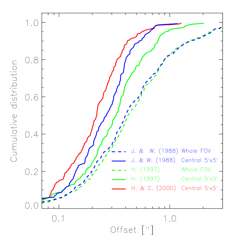
Figure 2: Cumulative distributions of offsets between X-ray and optical positions, for three optical catalogues: Jones & Walker (1988); Hillenbrand (1997); Hillenbrand & Carpenter (2000). For the first two, we show separate distributions for the inner $5^{\prime}\times 5^{\prime}$ and for the entire FOV. Since the third catalog covers only the central region, a single distribution is shown.

In order to verify that the probability of spurious identification is small, we calculated the expected number, $N_{ch.id}$, of chance correlations in a given region of our image by estimating the object surface density at the positions of our sources ($\rho_{obj}$), multiplying these densities by the coincidence region areas ($A_{id}$) and then summing over all sources, i.e.:

$$N_{ch.id}=\sum_{i}{A_{id}^{i}\cdot\rho_{obj}^{i}}$$ (1)

where the sum is extended over all sources in the region of interest. To estimate the surface density $\rho_{obj}$, we characterised the FOV in two different ways: as square tiles of $1^{\prime}$ on a side, and as a series of concentric annuli centered on the X-ray field, with the radius of each annulus $0.5^{\prime}$ greater than that of the previous one. We then counted the number of cataloged sources in each of these regions and divided by their area. The two methods gave equivalent results. The probability of chance identification is highest in the field center, $\sim 5\%$ for the inner $1^{\prime}$ radius; for the entire field, the chance probability is $\sim 2\%$. If anything, these probabilities could even be smaller, since actual identification radii for most optical catalogues were smaller than the conservative $0.75^{\prime\prime}$ used here.

We can compare these estimates with the number of spurious X-ray sources expected on the basis of the SNR threshold chosen for detection (cf. §2.2). With 10 such spurious detections expected in the full FOV, none (i.e., $\lesssim 0.2$) will be associated by chance with a known object. This means we needn’t worry about spurious sources when studying the properties of previously cataloged objects. When exploring the nature of unidentified sources (cf. Paper II), however, we must remember that $\sim 10$ detections will be spurious.

We can also estimate the number of times an X-ray source identified with its true counterpart will be identified by chance with a second object. Assuming that the object positions are uncorrelated, we multiply the fraction of chance identifications (2%) by the total number of sources (742) to get an expected $\lesssim 15$ double chance identifications in the entire field. Since we actually find 50 multiple ID’s, the source positions probably are correlated.

3.3 Physical properties of cataloged stars

For each object in our merged catalog we collected relevant data such as X-ray count rates, optical and IR photometry, rotational periods, etc. In cases of redundant information, only one of the available values was chosen: the last column of Table 2 reports the information used from each catalog, and in cases of redundant information, a superscript on a quantity indicates the precedence rank with which values were adopted for our merged list (e.g., $H^{5}$ was used only if the other four catalogues with $H$ values had no entry for a given object). Table 3 gives the number of objects in our catalog for which we retrieved several measured or estimated quantities, as well as the same number referred to HRC sources identified with a single optical/IR object. The most complete data for objects are the near-IR $H$ and $K$ magnitudes, since the majority of the ONC population is embedded in the molecular cloud and is only detectable at IR wavelengths where the extinction ($A_{K}\sim 0.1A_{V}$) is greatly reduced from that in the optical.

A first look at our stars via IR photometry is shown in Figure 3 as a $K$ vs. $H-K$ diagram for the 763 stars in the inner $5^{\prime}\times 5^{\prime}$ of the FOV. The same diagram for the entire HRC FOV would be similar but, with 2431 stars, it would be overcrowded. X-ray sources are depicted with filled symbols and optically well characterized stars are shown with larger, open circles. Also shown are the main sequence and a 1 Myr. isochrone derived by transforming the evolutionary tracks of Siess, Dufour, & Forestini (2000, hereafter SDF) from the theoretical ($L_{bol}$ vs. $T_{eff}$) to the observational plane using the transformations of Bessell (1991) and Houdashelt et al. (2000). Reddening vectors for 1 Myr stars of three different masses are indicated by dashed lines. We cannot derive precise information on the nature of our stars from this diagram alone: $H$ and $K$ band magnitudes are indeed expected to be influenced by the presence of disks around many of our stars. We expect that stars with disk will be displaced with respect to those without disks toward the upper right of Figure 3. For 813 stars in common with our sample, Hillenbrand et al. (1998) derive a mean $I_{c}-K$ color excess of 0.36 magnitudes, with a standard deviation of 0.72 mag. Given that disk emission is expected to be minimum at $I$ band wavelengths, these values can be taken as a rough measure of the average $K$ band excess and as an upper limit to the $H-K$ color excess. We can conclude that the positions of stars in Figure 3, although influenced by excesses, are approximately representative of their photospheres. We then observe that our near IR catalog contains stars down to very low masses ($M<<0.1M_{\odot}$) and high extinction ($A_{V}>50$), and that stars are detected in our HRC data down to $M\gtrsim 0.1M_{\odot}$ and to quite high extinction ($A_{V}\sim 40$).

Table 3: Numbers of objects with each optical/IR data item

	$Spec.~{}~{}Type$	$A_{V}$	$L_{bol}$	$T_{eff}$	$Mass$	$Age$	$P_{rot}$	$Memb$
Whole sample	1001	924	907	908	900	873	451	1028
HRC detections	460	437	437	437	434	427	242	492
	$\Delta_{I-K}$	$EW_{CaII}$	$V$	$I$	$J$	$H$	$K$	$L$
Whole sample	785	872	1176	1625	2339	2532	2466	132
HRC detections	389	385	501	596	604	642	641	49

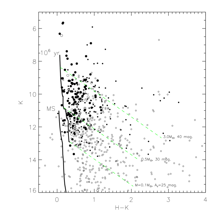
Figure 3: Near-IR color magnitude diagrams for the central $5^{\prime}\times 5^{\prime}$ of the HRC FOV. Large and small symbols indicate stars belonging and not belonging to the optical sample (see §3.4). Filled and empty symbols indicate objects unambiguously detected and not detected, respectively, in the HRC data. Also shown are the main sequence and the 1 Myr isochrone according to SDF evolutionary tracks.

One of our main goals, to be pursued further in Paper II, is to study the activity of young stars as a function of their mass and evolutionary stage. The most relevant data in this context are those given in the papers by Hillenbrand (1997) and Hillenbrand et al. (1998). The largest part of our spectral types, extinction estimates ($A_{V}$), $T_{eff}$ and $L_{bol}$ measurements are taken from Hillenbrand (1997), and we refer the reader to that work for details. The same author also derives stellar masses and ages using the D’Antona & Mazzitelli (1994) evolutionary tracks. Since new improved model calculations have been published, we decided to estimate masses and ages anew from the published temperatures and luminosities. We considered two sets of calculations: those by D’Antona & Mazzitelli (1997, hereafter DM97) ($Z=0.02$, $Y=0.28$, $X_{d}=2\times 10^{-5}$) and those of SDF ($Z=0.02$, $Y=0.277$, $X=0.703$ and no overshooting). Recent estimates of dynamical masses for seven single stars and two binary systems by Simon, Dutrey, & Guilloteau (2000) seem to favor the SDF over the DM97 tracks. We also observe that for ONC members the SDF tracks produce a smaller age spread than do the DM97 calculations, possibly better reflecting the real star formation history. Given uncertainties in the models, it is premature to rely exclusively on a particular set of tracks. We primarily have adopted the SDF tracks and in Paper II will note whether and how our results are influenced by this choice over that of the DM97 calculations.

Masses and visual absorptions for 19 presumed brown dwarfs ($0.008\leq M/M_{\odot}\leq 0.08$) and 3 low mass stars studied with IR spectroscopy by Lucas et al. (2001) were used when available. For four of these objects we could also derive masses using the optical data of Hillenbrand (1997) and the SDF tracks: three are brown dwarfs ($M_{IR}=$ 0.073, 0.9074 and 0.071 $M_{\odot}$) according to the IR data and very low mass stars ($M_{Opt.}=$ 0.11, 0.11 and 0.19 $M_{\odot}$) according to the optical estimate; the fourth is a very low mass star with $M_{IR}=0.3M_{\odot}$ and $M_{Opt.}=0.21M_{\odot}$.

3.4 Definition of stellar samples

About a third (907) of the cataloged objects can be placed on the HR diagram and belong to the well characterized population studied by Hillenbrand (1997) and Hillenbrand et al. (1998). We were able to estimate masses and ages for 877 of these stars that lie within the SDF tracks. Masses for nine massive stars ($M/M_{\odot}>6.0$) were taken from Hillenbrand (1997). For four stars in the SDF tracks (see §3.3) and for 18 other very low mass stars and brown dwarfs, we adopt values by Lucas et al. (2001). For the most part, the remaining cataloged objects ($\sim 2000$) are heavily obscured stars detected only in the near IR and for which we therefore have limited information.

Hillenbrand (1997) argues that her sample, which comprises most of our well characterized sample, is representative of the whole ONC population and differs only in that its location on the near side of the molecular cloud gives it low optical extinction. This is important for our study of X-ray activity (Paper II) because it ensures that our results will not be strongly biased. As expected in a flux limited sample, however, the brighter and more massive stars studied by Hillenbrand (1997) are actually seen to larger values of visual extinction than their lower mass counterparts. In order to minimize selection effects for our studies, we limited part of our analysis to stars with $A_{V}<3.0$.

For the following analysis we define two groups of stars, mainly on the basis of the amount of available information:

1) Our optical sample is comprised of stars in the HRC FOV for which we have a mass estimate, whose values of $A_{V}$ are less than 3.0, and which are either confirmed proper motion members or have unknown proper motion (cf. §3.4.1). For the 696 stars of this optical sample, Table 4 lists: sky position, mass, age, rotational period, Ca II line equivalent width, HRC basal count rate (see §5), X-ray luminosity and $L_{X}/L_{bol}$ (cf. §4 and §5). The analysis of X-ray activity that we present in Paper II is based on these data.

Table 4: Catalog of the ONC optical sample

$N.$	$Ra(2000)$	$Dec(2000)$	$Mass$	$Log(Age)$	$P_{rot}$	$EW(CaII)$	$Ct.Rate$	$Log(L_{X})$	$Log(L_{X}/L_{bol})$
	[$~{}h$ $~{}m$ $~{}s$]	[∘  ′  ′′]	$[M_{\odot}]$	[yr.]	[days]		[ks-1]	$[ergs\cdot s^{-1}$]
(1)	(2)	(3)	(4)	(5)	(6)	(7)	(8)	(9)	(10)
1	5 34 12.81	-5 28 48.28	0.72	6.46	…	1.60	$<$ 4.02	$<$ 30.24	$<$ -3.14
2	5 34 14.39	-5 28 16.77	1.74	6.87	…	2.00	27.39	31.21	-3.12
3	5 34 17.15	-5 29 04.45	0.23	4.71	…	0.00	$<$ 3.28	$<$ 30.57	$<$ -3.08
4	5 34 17.92	-5 33 33.45	0.43	6.04	3.19	1.80	4.59	30.23	-3.23
5	5 34 19.39	-5 27 12.04	1.86	6.79	…	4.00	$<$ 2.83	$<$ 30.04	$<$ -4.35
6	5 34 19.47	-5 30 19.99	1.19	6.20	…	-2.50	$<$ 3.62	$<$ 30.48	$<$ -3.42
7	5 34 20.64	-5 32 35.24	0.19	6.29	…	1.80	$<$ 3.75	$<$ 30.14	$<$ -2.70
8	5 34 20.72	-5 23 29.18	0.28	6.55	…	0.00	1.74	29.81	-2.96
9	5 34 20.92	-5 24 48.53	0.25	6.52	…	0.70	$<$ 2.56	$<$ 29.97	$<$ -2.78
10	5 34 22.32	-5 22 27.01	0.12	5.07	…	…	$<$ 2.40	$<$ 29.95	$<$ -3.08

Note. — The 696 entries of the full table are available on-line at: http://www.astropa.unipa.it/$\sim$ettoref/PaperI_tables.html

2) The IR sample is comprised of 2476 stars with measured $K$ band magnitudes. The IR sample includes most of the optical sample, with 680 of 696 stars in common. This sample very likely contains a large fraction of all the ONC members of stellar and brown dwarf mass, with the possible exception of a few deeply reddened stars located in small regions where the cloud absorbing column is greatest (see Paper II). The central region, which also coincides with a thicker part of the molecular cloud, has been surveyed in depth by Hillenbrand & Carpenter (2000) and Lucas & Roche (2000). The survey of Hillenbrand & Carpenter (2000) is believed better than 90% complete to $K\sim 17.5$, corresponding to a mass of $\sim 0.02M_{\odot}$ (for an age of 1 Myr).

Figure 4: HR diagrams for stars belonging to the optical sample and for other ONC members which we could place in the diagram; see legend for symbol meanings. We indicate with filled circles and small crosses the stars in these two groups that were detected in the HRC image. Dashed and solid lines, respectively, represent SDF evolutionary tracks for masses from 0.1 to $7.0M_{\odot}$ and isochrones for ages between $10^{5}$ and $10^{8}$ years (note labels besides curves).

Figure 4 shows an HR diagram for the stars in our optical sample. We also show the positions of other confirmed proper motion members ($P_{memb}>50\%$) which are not part of the optical sample. For both groups we indicate stars (cf. figure legend) that are unambiguously identified with our X-ray sources. SDF tracks and isochrones used to estimate stellar masses and ages are also shown for reference.

In the following two sections we estimate the degree to which our two main stellar samples are contaminated by field objects not physically or spatially related to the ONC.

3.4.1 Contamination of the optical sample

In discussing the optical sample and its HR diagram we will make use of the membership information provided by Jones & Walker (1988). We consider three stellar subsamples that differ in confidence of their physical association with the ONC. The first, “group 0,” comprises all stars studied astrometrically by Jones & Walker (1988), regardless of membership probability as derived in that study. The next sample, “group 1,” comprises all stars with proper-motion membership probabilities greater than 50%. Thirdly, we consider the optical sample defined in the previous section, which excludes only those stars explicitly suspected of being non-members ($P_{memb}<50\%$).

We can estimate the number of field objects, $N_{field}$, that contaminates a (sub)sample of stars studied astrometrically (Jones & Walker, 1988) by interpreting proper motion probabilities literally: $N_{field}=\sum(1.0-P_{i})$, where $P_{i}$ is the probability that the $i^{th}$ object belongs to the ONC and the sum is extended over the whole (sub)sample. Table 5 displays our results, with the first two rows referring to stars in the entire HRC FOV and the inner $5^{\prime}\times 5^{\prime}$ region. The remainder of the table reports the full-field analysis as a function of stellar mass and age. The table gives total numbers of objects and field contamination fractions estimated for the stars in groups 0 ($P_{memb}$ known; columns 2 and 3) and group 1 ($P_{memb}\geq 50\%$; columns 4 and 5). The last two columns refer to the optical sample, which contains both stars with $P_{memb}\geq 50\%$ and stars with no proper motion information. For the former stars we estimate the fraction of field objects using the same procedure as for groups 0 and 1; for the latter, we assume that this fraction is the same as for group 0 (i.e., we use the values from column 3).

Regarding sample contaminations, we therefore draw the following conclusions: a) Field contamination for the whole sample is a factor of $\sim 2$ lower ($\sim 5\%$) in the central region with respect to the full FOV ($\sim 10\%$), most likely due to the high member surface density and to the optically opaque molecular cloud that effectively obscures background stars. b) Selection of stars with $P_{memb}\geq 50\%$ (i.e., group 1) reduces the contamination to $2-2.5\%$ regardless of the area considered. c) Contamination depends on position in the HR diagram, being highest for masses between 1 and 10$M_{\odot}$ and for the oldest stars ($Log(age)>6.5$) in group 0; this is likely the result of both the distribution of field stars in the observational HR diagram and of the dependence on mass and age of the member sky density (the $3-10M_{\odot}$ stars, for example, are the most uniformly distributed among the mass ranges considered and, given the centrally peaked member distribution, are found in regions of higher field star relative density). d) Contamination in the optical sample is probably not much larger than in group 1, our estimate being $3.5\%$ for the full FOV and $2.4\%$ for the central region. We therefore take the optical sample as our primary basis for the analysis of Paper II.

Table 5: Field star contamination for various samples

Sample	N(0)	Field % (0)	N(1)	Field % (1)	N(Opt)	Field % (Opt)
(1)	(2)	(3)	(4)	(5)	(6)	(7)
Whole FOV	1034	10.9	938	2.4	696	3.5
Inner $5^{\prime}\times 5^{\prime}$	241	4.6	235	2.2	138	2.4
	Mass and age breakdown
$M/M_{\odot}=0.10-0.16$	43	4.5	42	2.2	61	2.9
$M/M_{\odot}=0.16-0.25$	135	5.6	129	1.6	160	2.4
$M/M_{\odot}=0.25-0.50$	302	5.1	291	1.8	277	2.2
$M/M_{\odot}=0.50-1.00$	115	9.8	106	2.5	89	2.8
$M/M_{\odot}=1.00-2.00$	76	26.5	57	3.5	40	5.1
$M/M_{\odot}=2.00-3.00$	53	14.9	47	4.3	37	4.7
$M/M_{\odot}=3.00-10.00$	23	24.1	18	5.4	13	6.5
$M/M_{\odot}=10.00-50.00$	6	5.3	6	5.3	6	5.3
$Log(age)=4.50-5.50$	61	5.3	59	2.1	56	2.6
$Log(age)=5.50-6.00$	136	8.4	126	1.9	117	2.6
$Log(age)=6.00-6.50$	366	5.6	352	2.3	330	2.5
$Log(age)=6.50-7.50$	167	18.7	139	2.7	162	6.4

3.4.2 Contamination of the IR sample

For stars detected only in the $K$ band, we cannot perform the above estimates because of lack of proper motions or any other individual membership data. Nonetheless it is particularly important to have at least a statistical understanding of the contamination, since we expect deep $K$ band observations to begin to see through the dense molecular cloud.

We estimate the expected contamination by field objects (galactic and extra-galactic) with the following procedure. Briefly, we first determine a reasonable approximation to field objects surface density as a function of unabsorbed $K$ magnitude. Since the majority of field objects will be in the background with respect to the ONC, their density at a given magnitude will be lowered by absorption in the molecular cloud. A smaller, unabsorbed fraction will be in the foreground. We will assume that the shape of the $K$ distribution for the two populations is the same as that of the total field population. Second, in order to know the total number of contaminating non-members, we must estimate the ratio of the number of foreground to background stars. Thirdly, we use the ${}^{13}CO$ measurements published by Goldsmith, Bergin, & Lis (1997) to estimate the total molecular cloud absorption in $K$ ($A_{K}$) as a function of sky position. Note that because these data are only available in the field center the contamination can only be estimated in the central region. Fourth, we convolve the background star $K$ distribution with the $A_{K}$ distribution over the area of interest, and fifth, we add the unmodified foreground star distribution to obtain the expected density of the field stars as a function of $K$.

In the first step of the calculation outlined above, the field star density as a function of $K$ was derived from more than 13600 stars in the 2MASS survey within $1^{\circ}$ of the Trapezium: although this distribution is affected by the presence of the cluster and of the absorbing cloud, the vast majority of stars from which it is derived come from the field and are located off the cloud so that the final result will not be significantly affected. It is important to realize what the limiting magnitude of our $K$ band luminosity function is. Although the nominal 2MASS survey completeness limit in $K$ is 14.3, in many cases it goes fainter than this, and for the $1^{\circ}$-radius region considered here, the $K$ band luminosity function rises to $K\sim 15$ and turns over for fainter $K$ magnitudes. We will therefore take $K=15$ as our limit to the knowledge of the $K$ distribution. Considering that more than 90% of the area of interest has a ${}^{13}CO$ column density corresponding to $A_{K}>1.0$, we can confidently estimate background contamination down to $K\sim 16$.

In the second step above, where we estimate the fraction of foreground stars in the direction of the ONC and in a given solid angle, $f_{ONC}=N_{ONC}(d<470pc)/N_{ONC}(tot)$, we use the results obtained by Carpenter (2000) through the Wainscoat et al. (1992) galactic model. Although the author does not report a result for the ONC, he quotes a ratio of foreground to total field stars for Perseus, $f_{Per}=N_{Per}(d<320{\rm pc})/N_{Per}(tot)$, which has a similar galactic latitude ($b\sim-20^{\circ}$) to that of the ONC and a distance of 320 pc (vs. 470 pc). We assume that the object space density as a function of distance, $\rho(d)$, is the same in the two directions: with this assumption the fraction of foreground stars in the ONC can be expressed as:

$$f_{ONC}=f_{Per}\cdot\frac{\langle{\rho(470)}\rangle}{\langle{\rho(320)}\rangle}\cdot\left(\frac{470}{320}\right)^{3}\lesssim f_{Per}\cdot\left(\frac{470}{320}\right)^{3}$$ (2)

where $\langle\rho(d)\rangle$ is the mean stellar density within a distance $d$ and the last inequality is justified by the larger height of the ONC above the galactic plane. According to Carpenter (2000) $f_{Per}$ ranges from 0.05 to 0.08 in the $J$, $H$ and $K$ bands. We have (conservatively) taken the upper end of this range and scaled it by cube of the distances (eq. 2), therefore deriving $f_{ONC}\lesssim 0.25$. We will conservatively assume in the following that $f_{ONC}=0.25$; this could result in an overestimation of field contamination.

The fifth step of our calculation gives us the expected surface density of field stars in the central $5^{\prime}\times 5^{\prime}$ region as a function of magnitude. For example, we find a value of 0.16 stars ${\rm arcmin}^{-2}$ for $K<13$ and 0.44 stars ${\rm arcmin}^{-2}$ for $K<15$. These numbers can be compared with the observed mean densities in the same region at the same two limiting magnitudes: $\sim 21$ and $\sim 28$ stars ${\rm arcmin}^{-2}$ for $K<13$ and $K<15$ respectively. Even for $K<16$ the expected contamination from field stars is about 2%.

Having estimated the field star surface densities, we now compare our determinations with others, performed with similar data and in a similar fashion. Consider the densities of unabsorbed field stars. Carpenter et al. (2001), in their work on IR variability, derive an off-cloud density of 0.66 stars per square arcmin for $K<14.8$. Carpenter (2000) performs a similar calculation of the unabsorbed field star densities for the ONC and other clouds. From the author’s Figure 3, we can see that the mean field star density for $K<14.3$ at the galactic latitude of the ONC (i.e., -19 degrees) is about 0.5. The densities we derive are: 0.81 for $K<14.8$ and 0.64 for $K<14.3$, both within 20-30% of the previous derivations. Because our goal is to show that contamination is not significant, a more conservative approach is to adopt our slightly larger derivation for the stellar surface density. Comparing our expectation for the density of observed field stars with the results of Hillenbrand & Carpenter (2000), we find that their densities are about 50-60% lower than ours, in keeping with our conservative approach.

We conclude, therefore, that contamination in our IR sample is negligible in the center of the FOV down to $K\sim 16$. Note that this conclusion might not hold for the whole area under study, because of the lower average member densities and thinner background molecular cloud. The IR photometry in the outer regions is not as deep as in the center, however, so that even there, contamination is possibly not significant.

3.5 The BN/KL region

The BN/KL region, about $\sim 1^{\prime}$ northwest of the Trapezium, in the densest part of Orion Nebula Cloud, contains a cluster of massive embedded stars mostly observed in the IR. The X-ray emission of the IR sources in the region has been already investigated by Garmire et al. (2000) using Chandra ACIS-I data. We estimate, using PIMMS, that our HRC-I data is 1.5 to 4.0 times less sensitive, depending on the source $kT$ and $N_{H}$ (see §5.1), with the worst case corresponding to high absorptions ($N_{H}\sim 10^{23}$). With reference to the sky region depicted in Figure 6 of Garmire et al. (2000), our master catalog contains 61 distinct objects in the $\sim 0.6$ arcmin² area, 22 of which are detected by the HRC vs. 27 by ACIS (Table 2 in Garmire et al. 2000). Out of the five ACIS sources missed by the HRC three are classified as IR sources and two as X-ray only sources by Garmire et al. (2000). We do not detect the BN object itself, but our upper limit ($<12$ photons in 63 HRC-I ksec) is consistent with the low measured ACIS-I count-rate (18 photons in 48 ACIS-I ksec). The IR source ”n” (our source 272) likely varied between the time of the two observations: the HRC detects 49 photons while ACIS detects 61, which, assuming $N_{H}=10^{23}$ (Garmire et al., 2000) and $kT>1$ keV, indicates that the HRC luminosity is $\gtrsim 3$ time greater than that measured by ACIS. The IR source #17 in Table 2 of Garmire et al. (2000), our source 281 in table 1 was, with similar assumptions (but $N_{H}=10^{22.5}$), 6 times brighter in the HRC data. Two objects detected exclusively in X-rays, also appear to have varied: #16 (HRC source 284) being $\sim 3$ times brighter in the HRC; and # 23, undetected by the HRC and whose upper limit indicates a variation of at least a factor of 3.

4 Optical/IR properties of the HRC sources

In this section we discuss the K magnitude and estimated mass composition of the counterparts of our X-ray source sample. In doing so we often distinguish the two samples of optically characterized members and near-IR objects. In Paper II, following our study of correlations of X-ray activity with stellar parameters, we speculate on the possible nature of X-ray sources not identified with optical or IR counterparts.

The quantity most widely available for our cataloged objects is K band magnitude. In the upper panel of Figure 5 we show the K band magnitude distribution for all our cataloged objects together with that of the subsample of stars comprising our optical sample. Also shown are distributions referring to objects in these two samples that are detected in our HRC data and unambiguously identified with an IR or optical counterpart. The lower panel of the figure shows detection fractions of the two reference samples as a function of $K$. It can be seen that the fraction of objects detected in X rays is greater than 50% down to $K\sim 11$ but then decreases for fainter $K$ magnitudes, going to zero at $K\sim 14$ which roughly corresponds to the brown dwarf limit (cf. Figure 3) for 1 Myr-old unabsorbed stars. Similar results, although with slightly larger detection fractions, were obtained by Garmire et al. (2000) with their ACIS-I data. Optical sample stars follow a similar trend, although with detection fractions somewhat larger. A quantitative breakdown of detection fractions for several stellar samples and two limiting $K$ magnitudes is given in Table 6. Note the increased detection fractions in the center of the FOV.

Table 6: Detection fractions vs. K magnitude

	Sky region	$K\leq 11$	$K\leq 14$
IR sample	Full FOV	0.57	0.32
”	Central $5^{\prime}\times 5^{\prime}$	0.63	0.41
Optical sample	Full FOV	0.69	0.50
”	Central $5^{\prime}\times 5^{\prime}$	0.81	0.71
Optical sample (max )	Central $5^{\prime}\times 5^{\prime}$	0.90	0.77

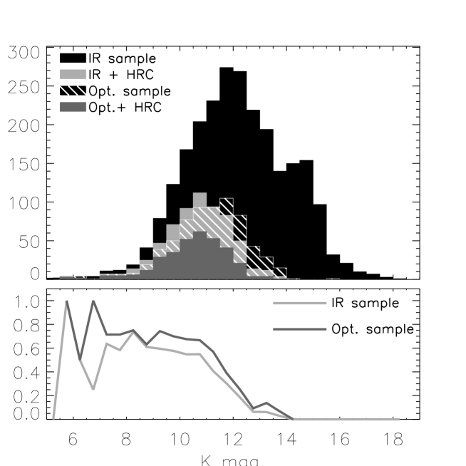
Figure 5: Upper panel shows K band distributions for: the IR sample (black), i.e., all objects within the HRC FOV with measured $K$ magnitudes; X-ray detected and unambiguously identified objects (light gray), the well characterized optical sample (cross-hatched, see text); and optical sample objects detected in X rays (dark gray). Lower panel displays HRC detection fractions for the IR and optical samples (light and dark gray, respectively) as a function of $K$ mag.

Figure 6 (upper panel) shows the distribution of stellar masses for our optical sample and the subset of X-ray detected stars. As in the previous figure, the lower panel shows the detection fraction: we see that the detection fraction is 100% for the most massive stars, drops abruptly for $Log(M/M_{\odot})=0.3-1.0$ ($M/M_{\odot}\sim 2.0-10.0$), rises again to about 90% and then decreases fairly smoothly to zero in the brown dwarf regime. A similar trend (not shown) is observed in the field center, although the detection fractions are 10-20% higher between $\sim 0.1$ and $\sim 2.0M_{\odot}$.

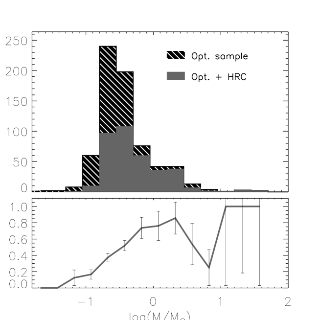
Figure 6: Upper panel: Mass distributions of objects in the HRC FOV and belonging to our optical sample. Shadings same as in Figure 5. Lower panel: Detection fraction vs. mass; error bars computed from Poisson statistics.

5 Determination of $L_{X}$ and $L_{X}/L_{bol}$ for HRC sources

Here we estimate two activity indicators, X-ray luminosity ($L_{X}$) and its ratio to bolometric luminosity ($L_{X}/L_{bol}$), and estimate their associated uncertainties. $L_{X}$ represents total coronal power output, while $L_{X}/L_{bol}$ is related to the fraction of total stellar energy that goes into heating the corona. In our search for physical mechanisms that may drive activity in young PMS stars, Paper II studies the relationship of these indicators with various stellar parameters.

Because the intensity of many of the HRC sources varied during our observation, we did not use mean count rates to estimate luminosities. Instead we have defined a basal count rate to remove the effects of short term ($\lesssim 63$ ksec) variability. Our basal rate algorithm searches for that count rate compatible with the largest possible portion of the light curve. Figure 7 shows five light curves of highly variable sources and their basal rates, and Table 4 lists our estimates for the basal count rates, $L_{X}$ and the ratio between $L_{X}$ and $L_{bol}$ for the stars in our optical sample.

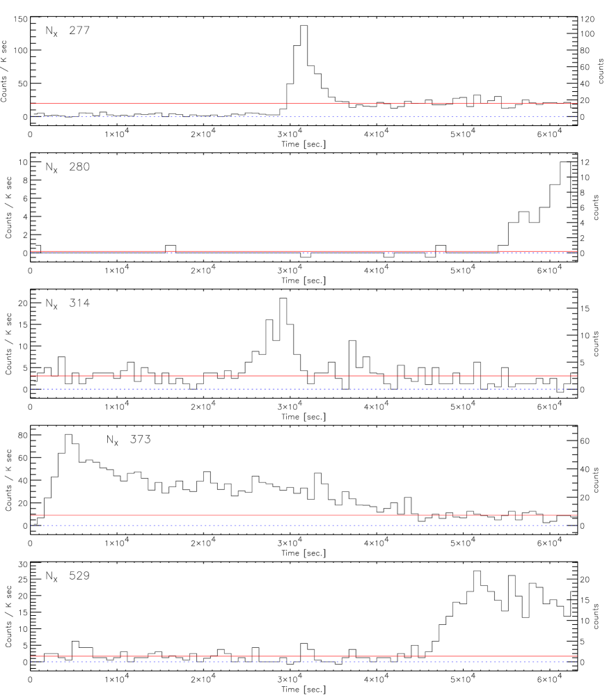
Figure 7: Light curves for five strongly variable HRC sources (number indicated at upper left of each panel) vs. time elapsed since observation start. Bin size varies from source to source, and left and right ordinate scales show count rates and counts per bin, respectively. Solid horizontal lines indicate derived basal rates (see text); dashed lines show zero levels. Source data were extracted from circular regions around each position, with subtracted background estimated from larger concentric annuli.

5.1 Chandra HRC count rate to flux conversion factors (CFs)

In order to convert basal count rates to intrinsic X-ray luminosity (assuming a distance of 470 pc), we have derived conversion factors (CFs) that yield unabsorbed source flux from observed count rate. We have assumed both that emitted radiation can be described as thermal, optically thin, emission from an isothermal plasma at temperature $kT$, and that the absorbing interstellar material along the line of sight can be characterized by a hydrogen column density $N_{H}$. We find that the X-ray flux of stars in our optical sample can be adequately described by an isothermal ($kT=2.16$) optically thin plasma, absorbed by a gas column density proportional to optical extinction: $N_{H}=2\cdot 10^{21}A_{V}$. This conclusion is based upon a spectral analysis of archival ONC X-ray data from the Advanced CCD Imaging Spectrometer (ACIS, Townsley et al. 2000), as discussed in Appendix A. Because the Chandra HRC lacks spectral resolution, $N_{H}$ and $kT$ values cannot be deduced from our main dataset alone.

In order to study the sensitivity of the conversion factor to the assumed plasma temperature and hydrogen column density we have explored the two dimensional ($kT$, $N_{H}$) parameter space in the range $kT<8.0$ and $20<Log(N_{H})<23$ which most likely include the conditions of the vast majority of our sources. All our HRC CFs are computed using PIMMS, a Raymond-Smith spectral model and a spectral band between 0.1 and 4.0 keV. Figure 8 shows a contour plot of the ratio of the conversion factor at a given $kT$ and $N_{H}$ within the specified ranges, to the conversion factor for typical ONC values of $kT=2.16$ and $N_{H}=3\cdot 10^{21}$. The plot shows that the dependence of the conversion factor on temperature and $N_{H}$ is quite weak for $kT>1.0$ and values of $N_{H}$ around the assumed value. The weak dependence of the CF on temperature justifies (at least for purposes of computing the CFs) the assumption of a single temperature instead of the full EM distribution. Provided the majority of emitting plasma is at temperatures larger than $\sim 1.0$ keV (likely for ONC PMS stars) and the estimates of $N_{H}$ are reasonable, our approach will give useful results.

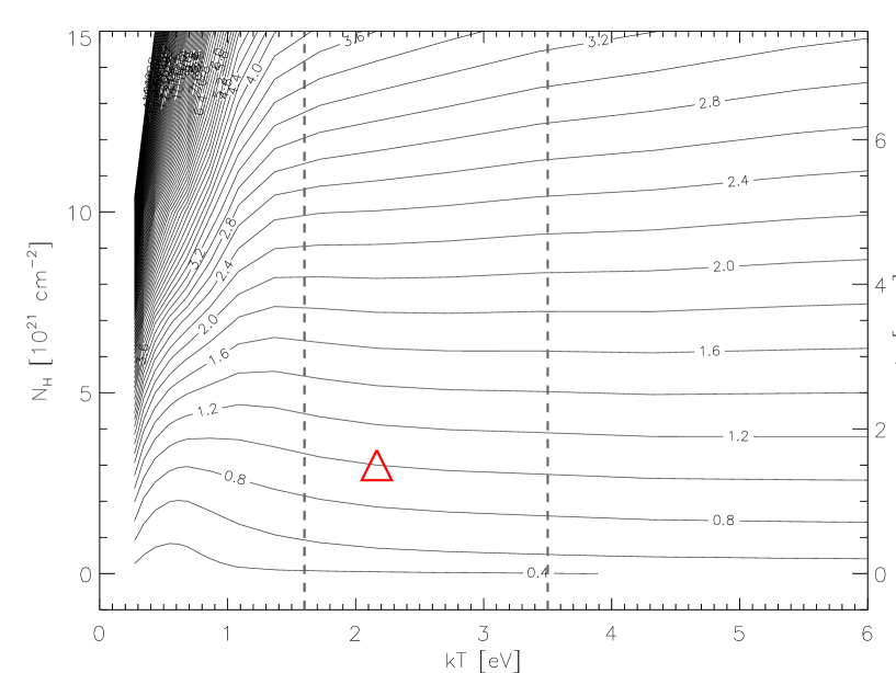
Figure 8: Contour plot of the ratio between the HRC conversion factor computed for $kT=2.16$ and $N_{H}=3\cdot 10^{21}$ ($2.9\cdot 10^{-11}ergs\ cm^{-2}$ per photon; denoted by large triangle) and the same conversion factor at different values of $kT$ and $N_{H}$. Right vertical axis gives the standard conversion between $N_{H}$ and $A_{V}$. Region between the two dashed vertical lines depicts likely range of ONC source temperatures.

The next step, for each of our sources, is to estimate a temperature representative of the emitting plasma and a value of $N_{H}$ quantifying the amount of interstellar gas between the source and the observer. If the range of such representative temperatures is such that $kT>1.0$ keV (cf. §A.2), we may safely use a single temperature ($\sim 2$ keV) to compute the CFs for all sources. Although this $kT$ is somewhat higher than 1 keV, a value often used in past X-ray studies of PMS stars, the HRC conversion factors we thus derive differ, for typical $N_{H}$, by at most $0.1$ dex. $N_{H}$, on the other hand, must be evaluated individually since it certainly spans a large range of values. We can estimate $N_{H}$ independently from X-ray information by using the standard linear correlation with the optical absorption: $N_{H}=2.0\cdot 10^{21}A_{V}$ (cf. Ryter, 1996). Adopting such a linear relation between optical absorption (due to dust grains) and gas column density (responsible for X-ray absorption) assumes that the gas to dust ratio is the same for all of our sources and equal to the value inferred for field stars. This assumption might not hold for the ONC members for two reasons: 1) most of the absorption is due to the molecular cloud in which the cluster is embedded rather than to interstellar matter between us and the cloud, and these two mediums might have different gas to dust ratios; and 2) the circumstellar environment of these PMS stars, many of which are actively accreting material from disks, is complex and might in principle contribute to an anomalous extinction law. An independent check on the validity and limits of the above assumption (see Appendix A) allows us to proceed in using this $N_{H}$-$A_{V}$ relationship to derive $N_{H}$ from the $A_{V}$ values of Hillenbrand (1997) for many of our ONC members. This is particularly applicable for stars in our optical sample that enter into the analysis of correlations between activity and stellar parameters (Paper II).

To summarize this discussion, as well as that of Appendix A, the conversion between count rates and energy fluxes or luminosities is a crucial step, usually requiring some spectral information. We have satisfied this need with archival ACIS data and conclude that our conversion factors are good to better than $\sim 30\%$ (0.1 dex), albeit with a 1$\sigma$ scatter of $\sim 0.2$ dex. This conclusion does not appear to depend on stellar mass or accretion rate.

5.2 Uncertainties on $L_{X}$ and $L_{X}/L_{bol}$

Uncertainties in our inferred X-ray luminosities are predominately due to the conversion from counts to flux (except for the weakest of our sources, where Poisson statistics are also important). In §5.1 we found that the statistical uncertainties on the CFs will be of the order of 0.2 dex (1 $\sigma$). Count rate measurements have a median fractional Poisson uncertainty of $\sim 17$% (+0.07, -0.08 dex), smaller compared to the total $L_{X}$ error, but for 5% (or 35%) of sources, this component is $\gtrsim 50$% (or 30%), comparable to the conversion factor uncertainty.

Distance uncertainties will also influence luminosity values. At 470 pc, the ONC’s angular extent ($\sim 30^{\prime}$) corresponds to $\sim 4$ pc, and the range of modern distance determinations introduces an additional systematic uncertainty of $\sim 30$ pc, together yielding $\Delta L_{X}\approx 13\%$. Since such largely systematic uncertainties won’t qualitatively influence our results for the dependence of coronal activity on stellar parameters, we neglect these.

The $L_{X}/L_{bol}$ ratio will be affected by uncertainties in both $L_{X}$ and $L_{bol}$. For stars in our optical sample we have adopted the $L_{bol}$ values of Hillenbrand (1997) with typical errors of $\lesssim 0.2$ dex (stars with strong circumstellar accretion could have slightly larger, underestimation errors). A quadrature sum of the uncertainties of $\sim 0.2$ dex for $Log(L_{X})$ and 0.2 dex for $Log(L_{bol})$ yields a total $Log(L_{X}/L_{bol})$ uncertainty of $\sim 0.3$ dex.

6 Summary

Our pwdetect wavelet algorithm finds 742 X-ray sources in the $30^{\prime}\times 30^{\prime}$ FOV of our 63 ksec Chandra HRC-I observation of the ONC. As a basis for our study of ONC X-ray activity (see Paper II), we have combined 17 different catalogs from the recent literature to assemble a catalog of all available information for nearly 2900 objects, the large majority of which are ONC members. We then calculated mass and age for a significant subset using the evolutionary tracks of Siess, Dufour, & Forestini (2000) and defined two reference stellar samples: the optical sample, comprising $\sim 700$ well characterized members with low extinction ($A_{V}\leq 3.0$), and the IR sample, largely including the optical sample and comprising $\sim 2500$ stars observed in the $K$ band. We have shown that field object contamination is quite limited in both of these samples.

In order to characterize the population of X-ray detected objects, we have presented distributions of $K$ magnitudes and masses and have noted, in agreement with the results of Gagné et al. (1995) and Garmire et al. (2000), a clear dependence of the percentage of detections on stellar mass, from $\sim 0$% at the brown dwarf limit, to $\sim 100$% for $\sim 2.0M_{\odot}$ stars. For 2 – 10 $M_{\odot}$ stars, detection fraction drops sharply, followed by a marked increase (to 100%) for the six highest mass ONC stars.

We concluded here by estimating activity indicators ($L_{X}$ and $L_{X}/L_{bol}$) for stars in our optical sample; Paper II studies correlations between this X-ray activity and other stellar parameters. Our X-ray luminosities were computed from basal count rates, assuming single temperature spectra for all sources and proportionality between X-ray absorption and optical extinction, with these assumptions verified by our analysis of medium resolution archival ACIS X-ray spectra for a subset of our sources.

Appendix A The ACIS data

On 1999 October 12-13, the Advanced CCD Imaging Spectrometer (ACIS, Townsley et al. 2000) observed the central region of the ONC for a total exposure time of $\sim 47$ ksec (“Obs ID” 18, Sequence No. 200016). These data were discussed by Garmire et al. (2000) and are available in the Chandra archive.

Here we utilize ACIS medium-resolution spectra to demonstrate that the fluxes of our HRC sources can be adequately described by an isothermal ($kT=2.16$) optically thin plasma, absorbed by a gas column density proportional to optical extinction: $N_{H}=2\cdot 10^{21}A_{V}$. This verifies the assumptions of §5 for a range of temperatures ($kT>0.5$ keV) and for adherence to the relationship between X-ray absorbing column and optical extinction.

Our spectral analysis characterized source spectra with two hardness ratios, $HR_{1}$ and $HR_{2}$, and compared the measured $HR$ pairs with model predictions for a grid of $kT$ and $N_{H}$ values. This approach is justified by the fact that large statistical uncertainties for the majority of our sample masks any (smaller) systematic inaccuracies introduced by our simplifying assumptions.

A.1 Data processing

In order to improve upon the standard energy calibration, we applied the correct_cti procedure (Townsley et al., 2000) to the Level 1 event file. This procedure (partially) corrects for the spatial nonuniformity of the ACIS spectral response that stems from degradation of the Charge Transfer Inefficiency (CTI) during the early days of the Chandra mission. With this correction, spectral resolution is $\sim$ 100-200 eV, depending both on the incidence position with respect to the readout node and on the photon energy. Following this correction we applied standard grade and status flag filtering to produce a “clean” Level 2 event file.

We then extracted background-subtracted source counts in three spectral bands: 0.5-1.7keV (L), 1.7-2.8keV (M) and 2.8-8.0keV (H), for 678 HRC sources that fell in the ACIS FOV. Source spectra were extracted from circles centered on the HRC source positions, with radius 3 times the HRC source size as measured by pwdetect (see §2.2). Background was estimated from concentric annuli of inner and outer radii of 4 and 5 times the HRC source size. To avoid contamination effects, we discarded 36 sources because of the proximity (distance $<$ 6 times the size) of another HRC source, and 150 additional sources were excluded due to net counts $\lesssim 0$ in one or more of the three spectral bands.

For the remaining 492 sources we calculated two hardness ratios defined as $HR_{1}=(M-L)/(M+L)$ and $HR_{2}=(H-M)/(H+M)$. Uncertainties on the hardness ratios were derived assuming that the number of source and background photons in each spectral band followed a Poisson distribution with mean equal to the measured value.

A.2 Interpretation

We computed hardness ratio predictions for a grid of isothermal Raymond-Smith models with a range of temperatures and hydrogen column densities, using PIMMS. Figure 9 shows the results of our PIMMS calculations in a grid of $HR_{1}$ vs. $HR_{2}$; also shown are positions of high SNR HRC sources (see caption). By interpolation in this plane, we can derive $kT^{HR}$ and $N_{H}^{HR}$, where the superscript refers to the method used to estimate these quantities. From these two spectral parameters we can derive the desired HRC conversion factors, $CF^{HR}$ (cf. Figure 8).

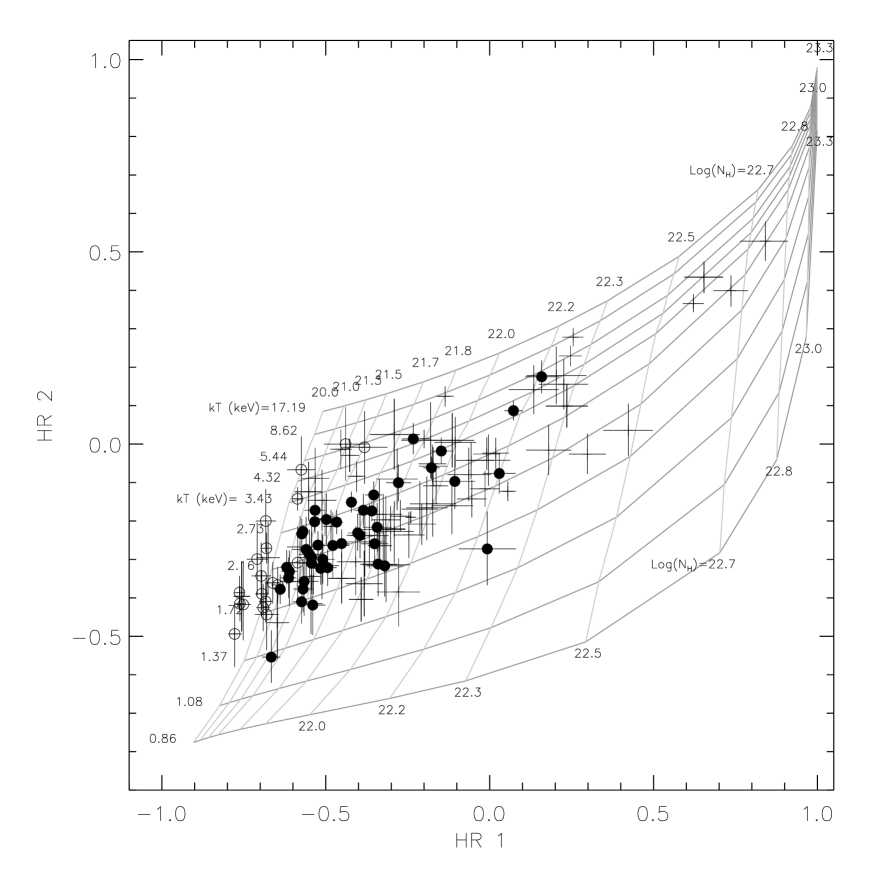
Figure 9: Grid of predicted ACIS hardness ratios for absorbed single-temperature Raymond-Smith models; kT ranges from 0.27 to 8.62 keV, with $Log(N_{H})$ running from 20 to 23.3. Filled circles denote optical sample stars that have hardness ratios and errors within the grid, and whose inferred values of $kT$, $N_{H}$ and HRC conversion factor were used for our analysis (see text). Open circles have HR values (or errors) near the grid edge, preventing their use. Pluses denote positions (and error bars) of HRC sources with computed errors of less than 0.1 for $HR_{1}$ and $HR_{2}$.

Formal $1\sigma$ errors on $kT^{HR}$, $N_{H}^{HR}$ and $CF^{HR}$ were derived (along with uncertainties on the hardness ratios) by Monte Carlo methods with the assumption that extracted source (and background) counts were Poisson distributed with mean equal to the measured value. In order to compute mean values and errors we require that the source has at least a 90% chance of lying inside the HR grid. For this reason a few points that lie inside the grid, but close to its boundaries are excluded from the subsequent analysis, along with those that lie outside. These latter points may be explained either by statistical fluctuation in the hardness ratio or by the fact that their spectra cannot be modeled as simply as we have assumed (e.g., they have a significant second temperature thermal component; this could explain the points on the left hand side of Fig. 9).

The majority of our sources have low SNR, in both the HRC and the ACIS datasets. This affects our hardness ratio analysis: the $1\sigma$ error bars are in general quite large. Examination of Figure 9 shows that (especially at very low and very high values) $kT^{HR}$ and $N_{H}^{HR}$ are quite strong functions of the two ratios, making it difficult to determine the two parameters. We therefore decided to include in the following conversion factor analysis only sources with errors on $HR_{1}$ and $HR_{2}$ less than 0.1, i.e., the subsample depicted in Figure 9. This choice is dictated by our interest in trends of median $CF^{HR}$ with mass, accretion, etc. By definition, the median is not weighted and does not take into account variable errors, and including a larger number of low SNR points would not necessarily improve the statistical significance of the median.

The median $kT^{HR}$ for our high SNR group is 2.2 keV with 90% of the sources in the 1.6-3.5 keV range. A fraction of this scatter can be explained by uncertainties on the hardness ratios: with the mean temperature as reference (i.e., $\sim 2.4$ keV), the formal $\chi^{2}$ is only 2.8. We examined trends in $kT$ with stellar mass and age, finding no significant evidence for a dependence in the range $0.2-10M_{\odot}$. Neither could we find any significant difference in the kT distributions of “high” and “low” accretion stars as defined from the Ca II equivalent width (cf. Paper II). Given the range of temperatures found and the discussion concerning Figure 8 (cf. §5.1), we can be assured that an error on the the assumed kT does not influence the HRC conversion factor by more than $\sim 10$%. Consequently, the most important aspect of our analysis becomes the study of the relation between $N_{H}^{HR}$ and $A_{V}$.

The mean ratio between $A_{V}$ and $N_{H}^{HR}$ is $0.54\cdot 10^{-21}$, not very different from the nominal value $0.5\cdot 10^{-21}$. However there are several objects that lie far from this mean relation so that the quartiles of the ratio distribution are $0.21\cdot 10^{-21}$ and $0.77\cdot 10^{-21}$. It is unclear whether this large spread of values is due to a real departure from the $N_{H}$ vs. $A_{V}$ mean relation (i.e., to an anomalous gas to dust ratio) or to other factors such as an oversimplified spectral model.

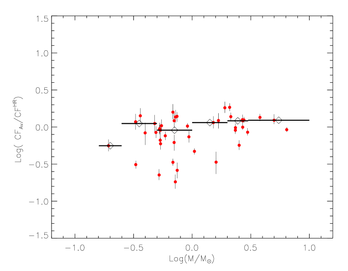
Figure 10: Ratio of HRC count rate to flux conversion factors vs. mass, computed from optical extinction and $kT=2.16$keV as described in the text. Only stars with high SNR are shown, with vertical error bars propagated from Poisson statistics. Horizontal segments with diamonds in their center represent median values of the points in the corresponding mass ranges (as employed in Paper II).

To conclude we examine the most important relation for our purpose: i.e., the relation between conversion factors derived from hardness ratios, $CF^{HR}$, and those derived assuming a constant temperature ($kT=2.16$) and $N_{H}$ proportional to $A_{V}$ ($CF_{A_{V}}$). The median for the logarithm of the $CF^{HR}/CF_{A_{V}}$ ratio is -0.024, and the $1\sigma$ quantiles are -0.252 and 0.130. Figure 10 shows this ratio as a function of stellar mass for our high SNR sample, as well as median values in the mass ranges defined in Paper II and depicted in the figure as horizontal segments. No significant trend in the median is apparent. We also considered separately samples of “high accretion” and “low accretion” stars, finding no difference in the conversion factor ratio; sample sizes for determining this latter comparison, however, are very small: nine “high accretion” stars vs. 14 with “low accretion” (cf. Paper II).

References

- Bally et al. (2000) Bally, J., O’Dell, C. R., & McCaughrean, M. J. 2000, AJ, 119, 2919
- Bessell (1991) Bessell, M. S. 1991, AJ, 101, 662
- Carpenter (2000) Carpenter, J. M. 2000, AJ, 120, 3139
- Carpenter et al. (2001) Carpenter, J. M., Hillenbrand, L. A., & Skrutskie, M. F. 2001, AJ, 121, 3160
- Damiani et al. (1997) Damiani, F., Maggio, A., Micela, G., & Sciortino, S. 1997, ApJ, 483, 350
- Damiani et al. (2002) Damiani, F. et al. 2002 (In preparation)
- D’Antona & Mazzitelli (1994) D’Antona, F. & Mazzitelli, I. 1994, ApJS, 90, 467
- D’Antona & Mazzitelli (1997) D’Antona F., Mazzitelli I., 1997, Mem. S. A. It. Vol. 68. No. 4 (G. Micela, R. Pallavicini, S. Sciortino eds.)
- Felli et al. (1993) Felli, M., Taylor, G. B., Catarzi, M., Churchwell, E., & Kurtz, S. 1993, A&AS, 101, 127
- Flaccomio et al. (2002) Flaccomio, E., Damiani, F., Micela, G., Sciortino, S., Harnden, F. R., Murray, S. S., Wolk, S. J. 2002, ??
- Gagné et al. (1995) Gagné, M., Caillault, J., & Stauffer, J. R. 1995, ApJ, 445, 280
- Garmire et al. (2000) Garmire, G., Feigelson, E. D., Broos, P., Hillenbrand, L. A., Pravdo, S. H., Townsley, L., & Tsuboi, Y. 2000, AJ, 120, 1426
- Giacconi et al. (1972) Giacconi, R., Murray, S., Gursky, H., Kellogg, E., Schreier, E., & Tananbaum, H. 1972, ApJ, 178, 281
- Goldsmith, Bergin, & Lis (1997) Goldsmith, P. F., Bergin, E. A., & Lis, D. C. 1997, ApJ, 491, 615
- Harnden et al. (2001) Harnden, F. R. Adams, N. R., Damiani, F., Drake, J. J., Evans, N. R., Favata, F., Flaccomio, E., Freeman, P., Jeffries, R. ., Kashyap, V., Micela, G., Patten, B. M., Pizzolato, N., Schachter, J. F., Sciortino, S., Stauffer, J., Wolk, S. J., Zombeck, M. V. 2001, ApJ, 547, L141
- Herbst et al. (2000) Herbst, W., Rhode, K. L., Hillenbrand, L. A., & Curran, G. 2000, AJ, 119, 261
- Herbst et al. (2001) Herbst, W., Bailer-Jones, C. A. L., & Mundt, R. 2001, ApJ, 554, L197
- Hillenbrand (1997) Hillenbrand, L. A. 1997, AJ, 113, 1733