Effects of wind on radiation spectra from magnetized accretion disks

Abstract

The effects of a wind on the emerging spectrum from an inefficiently-radiating accretion flow in a global magnetic field are examined, based on the analytic solution obtained recently by one of the present authors. The results exhibit the steepening of the negative slope appearing in the intermediate frequency range of bremsstrahlung spectrum and the decrease in the luminosity ratio of thermal synchrotron to bremsstrahlung, in accordance with the increasing wind strength. Both effects are due to a suppressed mass accretion rate in the inner disk, caused by a mass loss in terms of wind.

In order to demonstrate the reliability of this model, Sagittarius A^∗ (Sgr A^∗) and the nucleus of M 31, both of which have been resolved in an X-ray band by Chandra, are taken up as the best candidates for the broadband spectral fittings. Although the observed X-ray data are reproduced for these objects by both of the inverse-Compton and the bremsstrahlung fittings, some evidence of preference for the latter are recognized. The wind effects are clearly seen in the latter fitting case, in which we can conclude that a widely extending accretion disk is present in each nucleus, with no or only weak wind in Sgr A^∗ and with a considerably strong wind in the nuclear region of M 31. Especially in Sgr A^∗, the inferred mass accretion rates are much smaller than the Bondi rate, whose estimate has become reliable due to Chandra. This fact strongly suggests that the accretion in this object does not proceed like Bondi’s prediction, though its extent almost reaches the Bondi radius.

1 INTRODUCTION

The broadband spectrum of Sgr A^∗, from radio to hard X-ray bands, was reproduced fairly well for the first time by Narayan, Yi and Mahadevan (1995) based on an optically thin ADAF (advection-dominated accretion flow) model. In contrast to the standard accretion-disk model (Shakura & Sunyaev 1973), the optically thin ADAF model could reproduce the wide spread of the observed spectrum. Namely, the rather narrow peak in the radio band was explained by thermal synchrotron radiation from the inner part of a disk with relativistic temperature, and X-ray luminosity, by the bremsstrahlung from the whole disk. Another great advantage of this model is in its low efficiency in producing radiative fluxes. The latter feature could make the model possible to explain the low luminosity of Sgr A^∗ compared with that expected from a standard disk of about the Bondi accretion rate (see, e.g., Melia & Falcke 2001).

This type of models for optically thin ADAFs has been developed by many authors (e.g., Ichimaru 1977; Rees et al. 1982; Narayan & Yi 1994, 1995a, b; Abramowicz et al. 1995; Blandford & Begelman 1999). Since, in this category, the viscosity of the accreting plasma plays a dominant role in both energy dissipation and angular-momentum extraction processes, we call it the viscous ADAF model. The model looked successful in explaining the broadband spectra not only of Sgr A^∗ (Narayan, Yi & Mahadevan 1995; Manmoto, Mineshige & Kusunose 1997; and Narayan et al. 1998b), but also of Galactic X-ray sources and of low-luminosity active galactic nuclei (LLAGNs; for a review, see Narayan, Mahadevan & Quataert 1998a).

Meanwhile, if the presence of ordered magnetic fields in the nuclear regions of galaxies is taken seriously, anther type of optically thin ADAF model can be constructed (Kaburaki 2000, for brevity, K00). Since, in this model, the gravitational energy of accreting matter is liberated through the plasma’s electric resistivity it will be called the resistive ADAF model. Angular momentum, on the other hand, is extracted from the accreting matter by an ordered magnetic field that is penetrating the disk and is twisted, to a certain extent, by the rotational motion of the accreting matter. The observed spectrum of Sgr A^∗ could be reproduced also by this model (Kino, Kaburaki & Yamazaki 2000, for brevity, KKY) as satisfactorily as the viscous ADAF models could.

Recently, however, a fairly drastic change of the above stated situation has come with the appearance of the results of the X-ray telescope, Chandra. Owing to its high resolution, the apparent nuclear sources of a few nearby galaxies have been further resolved into several point sources including a true nuclear source in each case (e.g., Garcia et al. 2000 for M31; Baganoff et al. 2001a for Sgr A^∗). The intrinsic X-ray luminosity of these true nuclear sources are therefore considerably lower in fact, and moreover, their spectra have tuned out to be much softer than previously believed.

Especially, this softness of the spectra requires a critical reconsideration of the broadband spectral fittings of these objects by optically thin ADAF models, because this fact may exclude the hitherto accepted bremsstrahlung fitting to the X-ray band of the spectra. Further, as already been demonstrated by some authors (e.g., Quataert & Narayan 1999; Di Matteo et al. 2000), the presence of winds emanating from accretion disks can alter the ratio of X-ray luminosity to radio luminosity. Therefore, it is also necessary to include the presence of winds into the basic models based on which the spectral fittings are performed. In this context, the resistive ADAF model has been developed to include winds emanating from the disk surfaces (Kaburaki 2001, for brevity, K01).

The present paper is devoted to describe the general predictions on the broadband spectra radiated from such accretion disks as described by the analytic model of K01, and to report the results of applications to Sgr A^∗ and the nucleus of M31. Although Di Matteo et al. (2000) insist the presence of winds in the nuclei of some nearby elliptical galaxies on the basis of their broadband spectral fittings by a wind-version of the viscous ADAF model, the results are still uncertain because the X-ray fluxes they used are obtained by ASCA and hence the nuclear sources are not resolved (see also Quataert & Narayan 1999, for a Galactic X-ray transient and Sgr A^∗). We therefore restrict our applications only to such objects as have been resolved by Chandra and the results of observations have been open to the public.

2 RESISTIVE ADAF MODEL INCLUDING WINDS

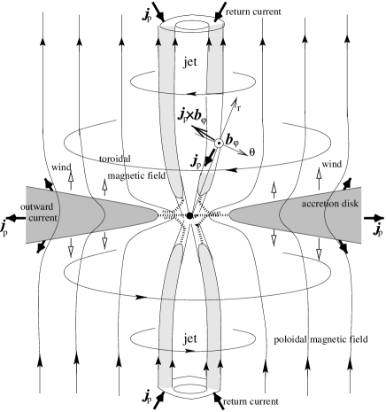
Figure 1: Conceptual drawing of the global configuration. The poloidal and toroidal components of the magnetic field lines are drawn with thin solid lines. The wind emanating from the disk surfaces and the poloidally circulating electric current are shown with white and black arrows, respectively. Also shown is the Lorentz force acting on the return current in the polar region, which has the components both for collimation and for radial acceleration of a jet. We distinguish jets from winds by their location and by the mechanisms for their launching.

In this section, we first introduce the basic ideas and physics contained in the resistive ADAF model proposed in K01, in which the presence of winds from the disk surfaces is allowed for. A schematic drawing of the global configuration presumed in the this model is given in Figure 1. An asymptotically uniform magnetic field is vertically penetrating the accretion disk and is twisted by the rotational motion of the plasma. Owing to the Maxwell stress of this twisted magnetic field, a certain fraction of the angular momentum of accreting plasma is carried out to infinity, and this fact ensures the plasma to gradually infall toward the central black hole.

In a stationary state, the deformation of magnetic field lines is determined by a balance between motional dragging and diffusive slippage of the field lines. Since the representative magnetic-Reynolds number $\Re$ is large (i.e., $\Re^{2}(r)\gg 1$) in the disk (except the region close to its inner edge, where $\Re\sim 1$), the deformations are also large. In this sense, the disk can be said as weakly resistive. Generally, the deformation in the toroidal direction is larger than that in the poloidal direction (i.e., $b_{\varphi}/b_{\rm p}\sim\Re$, where $b$ denotes the deformed part of the magnetic field).

The vertical structure of the disk is maintained by a pressure balance between the magnetic pressure of the toroidal field, which is dominant on the outside the disk, and the gas pressure in the disk: i.e., the accreting plasma is magnetically confined in a geometrically thin disk. Reflecting this fact, the gas pressure and density in the disk become quantities of order $\Re^{2}$ (see, equations [49] and [58] in K01). In general, this balance is not a static balance in its strict sense, and there may be a vertical flow from the upper and lower surfaces of a disk. We call such outflows (or inflows depending on the case) winds, distinguished from jets that may be formed within the inner edge of the accretion disk (also see below).

Since the wind velocity obtained in K01 is much smaller than the rotational velocity (by a factor of order $\sim\Delta\Re^{-1}$, where $\Delta\ll 1$ is the half-opening angle of the disk), its inertial force can hardly affect the vertical force balance described above. However, the wind may be accelerated, by some mechanisms with which we do not concern in this paper, to a considerable speed after it has been injected from the accretion disk to the wind region outside the disk. Here, we only expect that the upward wind proceeds to infinity because its total energy per unit mass (i.e., the Bernoulli sum in K01) is positive and hence the flow is unbound in the gravitational field.

The rotational velocity is a certain fraction of the Kepler velocity (i.e., a reduced Keplerian rotation) because the radial pressure-gradient force, together with the centrifugal force, sustains the gravitational pull on the plasma. In contrast to the rotational velocity, the infall velocity is a small quantity of the order of $\Re^{-1}$ as far as the disk is weakly resistive (i.e., except for the region near the inner edge). Their ratio does not depend on the disk thickness $\Delta$ as far as $\Re$ is regarded as a free parameter like the viscosity parameter $\alpha$ in the viscous ADAF models.

It has been demonstrated in K01 that, if the flow is completely adiabatic (i.e., if the liberated gravitational energy remains in each fluid element and is merely advected down the flow), the flow cannot drive winds. On the other hand, if some mechanism of energy transport (i.e., non-adiabaticity) allows the energy flow toward the accretion disk from the region within its inner edge, the disk can drive an upward wind. In K01, the presence of such mechanisms is treated implicitly in terms of a parameter $n$ that specifies the strength of a wind. The essence of the results is in that the presence of such non-adiabaticity affects solely on the radial profiles of the quantities such as density, pressure and magnetic field components (velocity components and temperature are not affected) but not on the vertical profiles. Thus, the presence of a wind appears unambiguously as a radius dependent mass accretion rate.

The analytic solution obtained in K01 describes the physical quantities in the accretion disk (i.e., the solution is valid only in between the inner and outer edges of the disk) with also a decreasing accuracy toward the upper and lower surfaces of the disk. The latter part of this statement means that the solution admits a few inconsistencies of the order of $\tanh^{2}\eta$, where $\eta\equiv(\theta-\pi/2)/\Delta$, in its variable-separated forms. These are negligible, however, except near the disk surfaces. Further, the solution does not care about the radiation loss. Nevertheless, since it has been confirmed retrospectively that the expected radiation flux from such a disk is negligibly small as far as the accretion rate is sufficiently smaller than the Eddington rate, the solution is consistent within this restriction. The disk spectrum can, therefore, be calculated with sufficient accuracy by using this solution, without any correction to the radiation losses.

If we extrapolate our physical understanding obtained within the disk even to the surrounding space, we are naturally led to the following picture of a galactic central engine. The engine is essentially a hydroelectric power station in which the ultimate energy source is the potential energy of the accreting plasma in the gravitational field. The accretion disk is a DC dynamo of an MHD type and drives a poloidally circulating current system, which is the cause of the toroidal magnetic component added to the originally vertical field (i.e., the twisting of the field lines). In the configuration shown in Figure 1, the radial current is driven outward in the accretion disk, and a part of the current closes its circuit through the near wind region while another part closes after circulating remote regions (probably reaching the boundary of a ‘cocoon’ enclosing hot winds). Anyway, these return currents concentrate within the polar regions in the upper and lower hemispheres, and finally return to the inner edge of the disk.

A bipolar jet may be formed from the plasma in this polar current regions, because the Lorentz force due to the toroidal field always has both of the necessary components for collimation and for radial acceleration, as shown in the figure. The often suggested universality of the association of an accretion disk and a bipolar jet is thus understood naturally in terms of one physical entity, the poloidally circulating current system. It is very likely that only a small fraction of the infalling matter input in the disk can actually fall onto the central black hole, with the remaining part expelled as a bipolar jet and a wind from disk surfaces.

3 SCALED QUANTITIES

The radial and co-latitude dependences of the all relevant quantities in the resistive ADAF solution are given in K01. In rewriting these quantities in a scaled form convenient for the discussion of LLAGNs, the following normalizations are adopted:

$$x\equiv\frac{r}{r_{\rm S}},\quad m\equiv\frac{M}{10^{8}M_{\odot}},\quad\dot{m}\equiv\frac{\dot{M}_{0}}{\dot{M}_{\rm c}},\quad b\equiv\frac{|B_{0}|}{1G},$$ (1)

where $r$, $M$, $\dot{M}_{0}$ and $B_{0}$ denote the radial distance, black-hole mass, mass accretion rate at the disk’s outer edge, $r=r_{\rm out}$, and strength of the external magnetic field at $r_{\rm out}$, respectively. The radius is normalized by the gravitational radius of the central black hole (actually neglecting its rotation, by the Schwarzschild radius $r_{\rm S}$) and the accretion rate, by the critical accretion rate defined in terms of the Eddington luminosity $L_{\rm E}$ as $\dot{M}_{\rm c}\equiv L_{\rm E}/(0.1c^{2})$, taking into account a typical conversion efficiency of $0.1$.

Further, we eliminate $|B_{0}|$ by the aid of the relation (see K01)

$$r_{\rm out}=\left(\frac{3\Re_{0}^{4n}}{2n+1}\ \frac{GM\dot{M}_{0}^{2}}{B_{0}^{4}}\right)^{1/5},$$ (2)

or

$$\quad b=7.6\times 10^{4}\ (2n+1)^{-1/4}\Re_{0}^{n}x_{\rm out}^{-5/4}\dot{m}^{1/2}m^{-1/2},$$ (3)

where $G$ is the gravitational constant. This is because $B_{0}$ seems rather difficult to infer from observations compared with the outer edge radius $r_{\rm out}$. Substituting the latter expression into the radial part of the variable-separated forms of the relevant quantities, we finally obtain

$$\tilde{v}_{\varphi}(x)=1.2\times 10^{10}\ (2n+1)^{1/2}x^{-1/2}\quad{\rm cm}\ {\rm s}^{-1},$$ (4)

$$\tilde{\rho}(x) = 1.5\times 10^{-12}\ (2n+1)^{-1/2}\Re_{0}^{2(n+1)}$$ (5)

$$\times x_{\rm out}^{-(1/2+2n)}\dot{m}m^{-1}x^{-(1-2n)}\quad{\rm g}\ {\rm cm^{-3}},$$

$$\tilde{p}(x) = 2.3\times 10^{8}\ (2n+1)^{-1/2}\Re_{0}^{2(n+1)}$$ (6)

$$\times x_{\rm out}^{-(1/2+2n)}\dot{m}m^{-1}x^{-2(1-n)}\quad{\rm dyne\ cm}^{-2},$$

$$\tilde{T}(x)=9.0\times 10^{11}x^{-1}\quad{\rm K},$$ (7)

$$|\tilde{b}_{\varphi}(x)| = 7.6\times 10^{4}\ (2n+1)^{-1/4}\Re_{0}^{n+1}$$ (8)

$$\times x_{\rm out}^{-(1/4+n)}\dot{m}^{1/2}m^{-1/2}\ x^{-(1-n)}\quad{\rm G},$$

and further,

$$\tau_{\rm es}(x)=3.7\times 10^{1}\ (2n+1)^{-1/2}\Re_{0}x_{\rm out}^{-(1/2+2n)}\dot{m}x^{2n},$$ (9)

$$\dot{M}(x)=\dot{M}_{0}x_{\rm out}^{-2n}x^{2n},$$ (10)

$$\Delta=\Re_{0}^{-(2n+1)},$$ (11)

where $v_{\varphi}$, $\rho$, $p$ and $\Delta$ are the rotational velocity, density, gas pressure and the half-opening angle of the disk, respectively, and the tildes above them denote their radial parts. The opacity is dominated by the electron scattering, and the resulting optical depth in the vertical direction $\tau_{\rm es}(x)$ depends on the radius like $x_{\rm out}^{-2n}x^{2n}=(r/r_{\rm out})^{2n}$. Therefore, it is much smaller than unity as far as $\dot{m}\ll 1$ and $x_{\rm out}\gg 1$ since $r/r_{\rm out}<1$. We can confirm the explicit dependence of the accretion rate on the radius in equation (10).

Since the radii of inner and outer edges are mutually related by $x_{\rm in}=\Re_{0}^{-2}x_{\rm out}$ (see K01), they are written in the present units as

$$r_{\rm out} = 3.0\times 10^{13}\ x_{\rm out}m\quad\mbox{cm},$$

$$\qquad r_{\rm in} = 3.0\times 10^{13}\ \Re_{0}^{-2}x_{\rm out}m\quad\mbox{cm}.$$ (12)

Although the numerical values appearing in the above scaled expressions are their formal values at the black hole horizon, a direct inward-extension of the above solution beyond the inner edge is meaningless because the solution becomes invalid there. Finally, we note that the number of free parameters contained in our solution is altogether 5, i.e., $m$, $\dot{m}$, $x_{\rm out}$, $\Re_{0}$ and $n$.

4 RADIATION PROCESSES

The method of calculating the expected spectrum from an accretion disk, based on the analytic solution of the resistive ADAF model including winds, is essentially the same as stated in KKY for the no-wind version of that model. The main radiation mechanisms are thermal cyclo-synchrotron emission most of which contributes to the flux in the radio band, thermal bremsstrahlung that may contribute mainly in the X-ray band, and inverse Compton scattering of the synchrotron (and bremsung) photons, which may appear as one or two peaks in the middle frequency range (and the scattered bremsung flux that may be scarcely recognized above the exponentially decaying part of the spectrum).

There are in the present scheme, however, two main differences from the former version. One is an improvement in the treatment of the Gaunt factor, and the other is in the approximation used in evaluating the unscattered (the sum of synchrotron and bremsung processes) flux from a disk. They are described in the following subsections. Hereafter, we need only the radial parts of the relevant physical quantities, and hence quote them without tildes on them for simplicity.

We first assume that an observed spectrum from a galactic nucleus is produced only by its accretion disk, and neglect the possible contributions from other components such as jet or wind. The validity of this assumption will be discussed in §5.3.

4.1 Unscattered Flux

Since the Compton unscattered flux consists of the synchrotron emission and the bremsung (both of which are assumed to be isotropic), the the absorption coefficient is calculated from Kirchhoff’s law

$$\alpha_{\nu}=\frac{\chi_{\nu,{\rm br}}+\chi_{\nu,{\rm sy}}}{4\pi B_{\nu}},$$ (13)

where $\chi_{\nu}$ denotes the volume emissivity for both processes and $B_{\nu}$ is the Planck function. Assuming LTE, we have for the specific intensity

$$I_{\nu}=B_{\nu}\left[1-\exp{(-\tau_{\nu})}\right],$$ (14)

where $\tau_{\nu}=\tau_{\nu}^{*}/\cos\theta$, $\tau_{\nu}^{*}=\alpha_{\nu}H$ and $H$ is the height of the disk.

In this situation, we approximate the emerging flux by an interpolation formula as

$$F_{\nu}\simeq\pi B_{\nu}\left[1-\exp{(-2\tau_{\nu}^{*})}\right].$$ (15)

This formula has a merit of giving the correct answers $\pi B_{\nu}$ and $(\chi_{\nu,{\rm br}}+\chi_{\nu,{\rm sy}})H/2$ in the optically thick and thin limits, respectively. The difference between this and the two-stream approximation adopted in KKY, however, remains small.

4.2 Bremsstrahlung

According to Narayan & Yi (1995b) and Manmoto, Mineshige & Kusunose (1997), KKY used the non-relativistic version of the Gaunt factor $g_{\rm ff}(\nu,T)$ not only for electron-ion collisions but also for electron-electron collisions, and a constant frequency-integrated Gaunt factor $g_{\rm B}(T)$. Compared with the more strict treatments of these quantities by Skibo et al. (1995), the old scheme evidently over-estimates the contribution from the e-e process when $h\nu<m_{\rm e}c^{2}$ (where $h$ is the Planck constant and $m_{\rm e}$ is the electron mass), and under-estimates it by about one order of magnitude when $h\nu>m_{\rm e}c^{2}$ (for more details, see Yamazaki 2002). Therefore, we adopt in this paper the formulae given by Skibo et al. (1995). The effect of this change on a spectrum is illustrated in Figure 7 (the thick and thin solid curves are calculated by the new and old versions, respectively, for the same fitting parameters).

In order to grasp the basic ideas, we first assume that the Gaunt factor is nearly constant even in the relativistic temperature regime. Then, the luminosity due to bremsstrahlung is roughly written as

$$L_{\nu}^{\rm bs}\propto\int_{r_{\rm in}}^{r_{\rm out}}\rho^{2}T^{-1/2}\exp[-h\nu/k_{\rm B}T]\ dV\propto f\ \Re_{0}^{2n+3}\dot{m}^{2}m,$$ (16)

where $k_{\rm B}$ is the Boltzmann constant, $dV=4\pi\Delta r^{2}dr$ is the volume element in the disk, and

$$f\equiv\int_{x_{\rm in}}^{x_{\rm out}}x^{1/2+4n}\exp[-h\nu/k_{\rm B}T(x)]\ dx.$$ (17)

Properly evaluating this integral $f$ in each of the typical frequency ranges, we have the frequency dependence

$$f\propto\cases{\mbox{const.}:&$\qquad\nu\ll k_{\rm B}T_{\rm out}/h$\cr\nu^{-3/2-4n}:&$\qquad k_{\rm B}T_{\rm out}/h<\nu\ll k_{\rm B}T_{\rm in}/h$\cr\exp[-h\nu/k_{\rm B}T_{\rm in}]:&$\qquad\nu>k_{\rm B}T_{\rm in}/h.$\cr}$$ (18)

In fact, however, in addition to the above features, there may appear an increase in the luminosity in the frequency range $\nu\sim k_{\rm B}T_{\rm in}/h$, which is due to the increase of the Gaunt factor at relativistic temperatures (see the peak B^′ in Figure 3).

The predicted power-law index of the luminosity $\nu L_{\nu}^{\rm bs}$, i.e. $-1/2-4n$ on the frequency, in the intermediate frequency range ($k_{\rm B}T_{\rm out}/h<\nu\ll k_{\rm B}T_{\rm in}/h$) exhibits an explicit difference from the corresponding prediction by the viscous ADAF model including winds (Quataert & Narayan 1999), $1/2-2p$ (where $p=2n$). In the no-wind case ($n=p=0$), the former predicts a negative slope while the latter does a positive slope in the $\nu$-$\nu L_{\nu}$ diagram. This difference comes from the difference in the radial dependences of the density in the basic analytic solutions (K00 and Narayan & Yi 1994, respectively). In both models, the inclusion of a wind ($n>0$) equally reduces these values depending on its strength. This is because the presence of a wind reduces the contribution from the inner parts of a disk to the bremsstrahlung (since $\dot{M}\propto x^{2n}$), resulting in a reduction of the higher frequency side of the spectrum.

4.3 Synchrotron Emission

The adopted formulae for the calculation of synchrotron emission and inverse Compton scattering is the same as in KKY. This synchrotron formula is known to be accurate when the electron temperature $T_{\rm e}$ is in the range $10^{8}<T_{\rm e}<3\times 10^{10}$. This temperature range corresponds in our solution to the radius range of $30<x<10^{4}$. Since, however, the contribution from the lower temperature region ($x>10^{4}$) is negligibly small compared with that from the bremsung, we can extend our calculation even to such regions (until the effects of recombination on the bremsung becomes important), by safely truncating the cyclo-synchrotron emission.

The critical frequency under which the radiation becomes optically thick at a fixed $r$ is given (Narayan & Yi 1995b; Mahadevan 1997) by

$$\nu_{\rm c}\propto T^{2}(x)|B_{\varphi}(x)|\propto\Re_{0}^{n+1}x_{\rm out}^{-(1+4n)}\dot{m}^{1/2}m^{-1/2}x^{-(3-n)}.$$ (19)

Since $\nu_{\rm c}$ increases towards the inner edge, inner part of a disk is apt to be optically thick at a given frequency $\nu$, with a critical radius

$$x_{\rm c} \propto \Re_{0}^{(n+1)/(3-n)}x_{\rm out}^{-(1+4n)/(3-n)}$$ (20)

$$\times\dot{m}^{1/2(3-n)}m^{-1/2(3-n)}\nu^{-1/(3-n)}.$$

Anyway, there is a radius $x_{\rm p}$ near $x_{\rm in}$ whose contribution to the self-absorbed radiation is the largest so that the peak frequency is determined as $\nu_{\rm p}=\nu_{\rm c}(x_{\rm p})$.

Then, for the self-absorbed luminosity per frequency ($\nu_{\rm min}<\nu<\nu_{\rm p}$, where $\nu_{\rm min}=\nu_{\rm c}(x_{\rm out}$)), we have

$$L_{\nu}^{\rm abs}\propto\int_{r_{\rm in}}^{r_{\rm c}}\frac{\nu^{2}}{c^{2}}k_{\rm B}T\ 2\pi r\ dr\propto(x_{\rm c}-x_{\rm in})m^{2}\nu^{2}\approx x_{\rm c}m^{2}\nu^{2},$$ (21)

where the final expression is valid only in the frequency range $\nu\ll\nu_{\rm p}$ in which $x_{\rm c}\gg x_{\rm in}$. In the crude approximation in which $x_{\rm c}$ is regarded as a constant, the luminosity of the self-absorbed synchrotron emission is determined solely by the central mass $m$.

However, substituting the above estimation for $x_{\rm c}$ in equation (20), we have a more accurate dependence

$$L_{\nu}^{\rm abs} \propto \Re_{0}^{(n+1)/(3-n)}x_{\rm out}^{-(1+4n)/(3-n)}$$ (22)

$$\times\dot{m}^{1/2(3-n)}m^{(11-4n)/2(3-n)}\nu^{(5-2n)/(3-n)}.$$

The strongest dependence on the parameters is still on the central mass, and its power varies slightly from 1.80 to 1.85 for the variation of $n$ in the allowed range, from 1/2 to $-1/4$. The dependence on the other parameters are rather weak, and this fact is very favorable to determine, at least within the framework of the present model, the central mass from the spectral fittings of this self-absorbed part, without much ambiguity (however, see also §5.3). The power of $\nu$ also varies only slightly from 1.6 to 1.7 in the same range of $n$.

The main effect of a wind on the synchrotron spectrum is a reduction of its peak intensity (when $n>0$) according to the wind strength. This is because the synchrotron emission comes mainly from the inner most region of an accretion disk where the magnetic field is the strongest and the electrons are most energetic, so that the reduction of the accretion rate in this region due to wind loss causes a decrease in the optically thin part of the emission.

5 APPLICATIONS

As stated in the previous section, we can calculate the spectrum emanating from an accretion disk by specifying the values of five parameters, $m$, $\dot{m}$, $x_{\rm out}$, $\Re_{0}$, and $n$. In other words, we can determine these values from the process of spectral fitting only if we have enough data points distributed over the full range of the spectrum of a specific object. In the applications of our model to Sgr A^∗ and M 31, we first proceed with this spirit, and regard all five parameters as free fitting parameters.

In fact, however, there are other information independent of the spectral data. For example, the central black-hole masses are known for these objects fairly accurately by the observations based on the dynamics. In the case of Sgr A^∗, the Chandra observations provide us a good estimate of the Bondi accretion rate. In principle, the results obtained from a spectral fitting should not conflict with these additional informations. If, however, there are some discrepancies between them, it may offer some important information about the inadequacy of the present status of the basic model or of our general understanding. Such considerations will be given in §5.3.

5.1 Sgr A^∗

Chandra has resolved a weak source at the radio position of Sgr A^∗ within the accuracy of 0^′′.35 (Baganoff et al. 2001a). Its absorption-corrected luminosity in 2-10 keV band is $2.4_{-0.6}^{+3.0}\times 10^{33}$ ergs s^-1 and power-law fitted photon index is $2.7_{-0.9}^{+1.3}$. For the other observational data than this X-ray band, we use those compiled by Narayan et al. (1998b). For the sake of comparison, the ROSAT value is also plotted in Figures 2, 3 and 7 with an empty circle. Among the radio observations, the 86 GHz point with the highest resolution obtained by VLBI is taken most seriously in the following spectral fittings.

The most restrictive feature of the Chandra results to the spectral fittings is the softness of the X-ray spectrum whose most probable slope in the $\nu$-$\nu L_{\nu}$ diagram is negative, in contrast to the ROSAT observation in which the slope in a similar X-ray range is positive. Although a rapid X-ray flaring is reported (Baganoff et al. 2001b), we do not discuss it here because the event is a transient phenomenon localized in a small region of the accreting plasma.

One possible way of reproducing this negative slope by our model is to use the decreasing side of the first-order Compton peak. Hereafter, we call this type of fittings the ‘Compton fitting’. In order for this negative slope to reach the Chandra X-ray band, the optically thin (i.e., the high frequency) side of the synchrotron peak should be located in a high enough frequency range. Nevertheless, the location of its self-absorbed (i.e., the low frequency) side is fixed by the 86 GHz point. Thus, the synchrotron peak in this fitting is required to be wide enough. Also, in order to keep the required X-ray luminosity, we require a sufficiently high luminosity to the synchrotron peak. However, these two requirements apt to contradict with the upper limit data in IR band, and hence the Compton fitting becomes very tight. We do not include wind in this type of fittings, because its inclusion does not cause any change in the overall spectral shape but reduces the luminosity only similarly at every frequency.

Actually the above stated requirement allows only a unique fitting, which is shown in Figure 2 with the full curve. The contribution from bremsstrahlung is buried in the second Compton peak. This curve seems to be marginally fitted to the observational constraints. The curve traces the observational data points fairly well on the low frequency side of the radio peak except around its top, but the X-ray slope is nearly at its steepest limit. If we try to improve the fitting to the X-ray slope, it becomes impossible for the curve to go through the 86 GHz point.

In this fitting, the accretion rate $\dot{m}$ has to be reduced from the previously inferred value (KKY) to a considerably lower value in order to suppress the contribution from bremsstrahlung. The position of the low frequency side of the synchrotron peak is fixed by adjusting mainly the black hole mass $m$ (see Eq. [21] or [22]). The most effective parameter to shift the Compton peak-frequency is $x_{\rm out}$, and a shift toward the high frequency side means a reduction of $x_{\rm out}$. In order to avoid the appearance of the inner edge radii smaller than that of the marginally-stable circular orbit, the magnetic Reynolds number at the outer boundary, $\Re_{0}$, should stay at rather small values. Since the obtained ratio $x_{\rm out}/x_{\rm in}$ from this fitting is not so large, the amplification of the seed magnetic field $B_{0}$ by the sweeping and twisting effects of the accretion flow remains to be rather small. In other words, this case of Compton fitting requires considerably large external magnetic fields, since $b_{\varphi}(x_{\rm in})$ is almost fixed by the height of the synchrotron peak.

The resulting values of the fitting parameters are summarized in Table 1. When a figure is expressed as three-digit number, it means that a change in the final digit causes a noticeable shift of the fitting curve. The dimension-recovered values and related physical quantities of our interest are

$$M=6.0\times 10^{5}\ M_{\odot},\quad\dot{M}_{0}=9.6\times 10^{-9}\ M_{\odot}\ \mbox{yr}^{-1},$$

$$r_{\rm out}=1.8\times 10^{13}\ \mbox{cm},\quad r_{\rm in}=1.2\times 10^{12}\ \mbox{cm}=6.8\ r_{\rm S},$$

$$|B_{0}|=2.7\ \mbox{G},\quad|b_{\varphi}(r_{\rm in})|=1.5\times 10^{2}\ \mbox{G},$$

$$\Delta=2.60\times 10^{-1}\ \mbox{rad}.$$ (23)

Another type of possible fittings is called the ‘bremsstrahlung fitting’, in which the Chandra spectrum is reproduced by the intermediate frequency range of the bremsstrahlung (Eq. [18]). In order for the Chandra frequency band to fall in this negative slope region, we have to take the disk’s outer edge $x_{\rm out}$ so large that its temperature decreases below about 1 keV. This corresponds to the outer edges of $x_{\rm out}>10^{5}$, and these values make a great contrast with the former value of $2.6\times 10^{3}$, that was obtained in KKY in reproducing the positive X-ray slope of ROSAT result by the low frequency range of the bremsstrahlung. The relatively faint X-ray luminosity of Chandra means a fairly small $\dot{m}$ also in this case, but not so extremely as in the Compton fitting case.

Two good examples of such fittings are shown in Figure 3. The full curve is for a no-wind case, and the dashed curve is for a weak-wind case. Although the fitting to the X-ray slope is much improved by the inclusion of a weak wind, the fitting to the low frequency side of the synchrotron peak becomes rather worse around its top. At present, we cannot clearly point out which is the best fit to Sgr A^∗, because of the lack of data points that are effective to distinguish them. High resolution observations in sub-millimeter to IR band would be very useful not only for this purpose but also to decide the superiority between the Compton and bremsung fittings.

The values of the fitting parameters obtained for each case are cited in Table 1, and the resulting values for the physical quantities are

$$M=4.0\times 10^{5}\ M_{\odot},\quad\dot{M}_{0}=3.7\times 10^{-8}\ M_{\odot}\ \mbox{yr}^{-1},$$

$$r_{\rm out}=1.2\times 10^{16}\ \mbox{cm},\quad r_{\rm in}=3.4\times 10^{12}\ \mbox{cm}=2.9\times 10^{1}\ r_{\rm S},$$

$$|B_{0}|=1.4\times 10^{-3}\ \mbox{G},\quad|b_{\varphi}(r_{\rm in})|=2.8\times 10^{2}\ \mbox{G},$$

$$\Delta=1.70\times 10^{-2}\ \mbox{rad},$$ (24)

for the solid curve, and

$$M=4.0\times 10^{5}\ M_{\odot},\quad\dot{M}_{0}=2.0\times 10^{-8}\ M_{\odot}\ \mbox{yr}^{-1},$$

$$r_{\rm out}=1.2\times 10^{16}\ \mbox{cm},\quad r_{\rm in}=1.6\times 10^{12}\ \mbox{cm}=1.3\times 10^{1}\ r_{\rm S},$$

$$|B_{0}|=1.6\times 10^{-3}\ \mbox{G},\quad|b_{\varphi}(r_{\rm in})|=4.2\times 10^{2}\ \mbox{G},$$

$$\Delta=4.71\times 10^{-3}\ \mbox{rad},$$ (25)

for the dashed curve.

In order to maintain a relatively higher synchrotron luminosity compared with the X-ray luminosity in the spectrum of Sgr A^∗, considerably large values are required for $\Re_{0}$ (i.e., small values for $\Delta$), and this fact results in reasonably small values for $x_{\rm in}$ in spite of large $x_{\rm out}$. The latter fact (i.e., $x_{\rm in}\ll x_{\rm out}$), in turn, guarantees the appearance of a well extended negative-slope region in the spectrum, and comfortably small values for the external magnetic field compared with the case of Compton fitting. The total bremsstrahlung hump in such a case shows a double-peaked structure in which the second peak (B^′ in Figure 3) on the higher-frequency side is emphasized by the enhancement of the Gaunt factor in the relativistic temperature regions located in the inner part of the disk (see also Figure 7).

The results in this case, therefore, predict a fairly wide extent of the ADAF state up to $x_{\rm out}>10^{5}$ with also a fairly low accretion rate of the order of $\dot{m}\sim$ a few $\times 10^{-6}$. For the obtained black-hole mass of $\sim$ a few $\times 10^{5}M_{\odot}$, the former value corresponds to the size of $r_{\rm out}>10^{16}$ cm, which is in good agreement with the marginally resolved radius of 0.02 pc of the nuclear X-ray source (Baganoff et al. 2001a). The corresponding values of the mass accretion rate at the outer radius, $\dot{M}_{0}$, is $\sim$ a few $\times 10^{-8}M_{\odot}$yr^-1. In the weak wind case, this value is further reduced to $\dot{M}(r_{\rm in})=3.4\times 10^{-9}M_{\odot}$yr^-1 at the inner edge. Therefore, these values are consistent with the limit $\leq 10^{-8}M_{\odot}$yr^-1 recently imposed on $\dot{M}(r_{\rm in})$ (Agol 2000; Quataert & Gruzinov 2000) from the interpretation of polarization measurement in the radio emission (Aitken et al. 2000, however see also Bower et al. 2001).

5.2 M 31

The nuclear source observed by ROSAT at the center of M 31 has also been resolved into five point sources by Chandra (Garcia et al. 2000). The true nuclear source is identified with that located within 1^′′ of the supermassive black hole and has an anomalously soft spectrum. They report that its luminosity in the 0.3-7.0 keV band is $4.0_{-2.8}^{+12}\times 10^{37}$ erg s^-1 and the power-law fitted photon index is $4.5\pm 1.5$ in the 0.3-1.8 keV range (we assume this value to hold up to 7.0 keV), after corrected for interstellar absorption. Although there seems to be some debates about these results, we tentatively fit our model to this observation.

Other observational data are obtained by VLA (Crane et al. 1992, 1993), IRAS (Soifer et al. 1986; Neugebauer et al. 1984), KPNO (McQuade, Calzelli & Kinney 1995), Palomar 5m telescope (Persson et al. 1980) and HST (Brown et al. 1998; King et al. 1995). The radio flux seems to have slight time variations. Among the HST data, the resolution of the $1.7\times 10^{15}$ Hz observation is much better ($\sim 0^{\prime\prime}.5$, King et al. 1995) than the other two (at 1.1 and 1.5 $\times 10^{15}$ Hz, Brown et al. 1998).

Although the available data points are rather few, the Compton fitting is very tight. Namely, if we try to adjust the fitting parameters such that the predicted curve passes through the radio and X-ray points (satisfying both luminosity and spectral index), it does automatically also the $1.7\times 10^{15}$ Hz point (Figure 4). Other HST and IR data should then be regarded as an excess whose origin may be attributed to other components than the ADAF under consideration. The fitted slope in the Chandra band seems somewhat harder, but it is the best we can do.

The determined fitting parameters are cited in Table 1, and the physical quantities of our interest are calculated as

$$M=7.0\times 10^{5}\ M_{\odot},\quad\dot{M}_{0}=5.6\times 10^{-7}\ M_{\odot}\ \mbox{yr}^{-1},$$

$$r_{\rm out}=3.7\times 10^{14}\ \mbox{cm},\quad r_{\rm in}=2.8\times 10^{12}\ \mbox{cm}=1.4\times 10^{1}\ r_{\rm S},$$

$$|B_{0}|=4.7\times 10^{-1}\ \mbox{G},\quad|b_{\varphi}(r_{\rm in})|=7.0\times 10^{2}\ \mbox{G},$$

$$\Delta=8.73\times 10^{-2}\ \mbox{rad}.$$ (26)

On the other hand, if we adopt the bremsung fitting, the fitting to the X-ray slope can be improved much more. In Figure 5, there are three curves that demonstrate the variations caused by the change in the wind parameter. Other parameters are adjusted in each curve to fit the radio, UV and X-ray luminosities simultaneously. As predicted in the previous section, we can clearly see the main effects of winds on the spectra, i.e., the steepening of the bremsung fall toward the high frequency side and the suppression of the synchrotron peak. For a more complete demonstration of such effects as caused by winds, we show in Figure 6 the variation of the spectrum according to the values of the wind parameter in its full range.

The values of the fitting parameters for each curve are summarized also in Table 1. The fitting to the X-ray slope seems satisfactory when $n$ is in between 0.3 and 0.5. However, it should be noted that the limiting case of $n=0.5$ corresponds to a flat density profile (i.e., it is independent of $x$; see Eq. [5]), which seems rather unplausible. The mass accretion rate in this fitting case increases by about one order of magnitude compared with Compton fitting case.

The resulting dimensional quantities in the case of thin solid curve ($n=0.3$), for example, are

$$M=4.0\times 10^{5}\ M_{\odot},\quad\dot{M}_{0}=2.7\times 10^{-6}\ M_{\odot}\ \mbox{yr}^{-1},$$

$$r_{\rm out}=5.3\times 10^{16}\ \mbox{cm},\quad r_{\rm in}=8.3\times 10^{12}\ \mbox{cm}=7.0\times 10^{1}\ r_{\rm S},$$

$$|B_{0}|=6.0\times 10^{-3}\ \mbox{G},\quad|b_{\varphi}(r_{\rm in})|=2.2\times 10^{2}\ \mbox{G},$$

$$\Delta=9.02\times 10^{-4}\ \mbox{rad}.$$ (27)

If we accept the bremsung fittings, we can conclude that M 31 has a considerably strong wind ($0.3<n<0.5$). However, it is again difficult to clearly insist the superiority of the bremsung fitting to the Compton fitting because of the shortage of the observational data points. High resolution observations at mm-waves are desirable for this purpose.

5.3 Discussion

In the previous subsections, we could reproduce the observed broadband spectra of Sgr A^∗ and M 31 fairly satisfactorily, by both of the Compton and bremsung fittings. Although some superiority of the latter case may be recognized in the fitting to the X-ray slope, it is difficult to say clearly which is the better one from the goodness of the fitting only. However, the preference becomes much more clear when we combine other information than from their spectra. In this course, the main issue relating to our basic model will also become evident.

The central dark mass of Sgr A^∗ is measured by the method of tracing stellar trajectories, and the result is $2.61\pm 0.35\times 10^{6}\ M_{\odot}$ within the inner 0.015 pc (Eckert & Genzel 1997; Ghez et al. 1998). On the other hand, the point mass obtained from our spectral fittings is almost one order of magnitude smaller than the ‘dynamical’ mass. For M 31, the central mass is estimated to be $3.3\times 10^{7}\ M_{\odot}$ by using HST photometry (Kormendy & Bender 1999). Also in this case, our model largely under-estimates it (apparently by about 30$\sim$40 times), even if the ambiguity caused by the shortage of data points is taken into account.

Since in our model the black hole mass is determined essentially by the fitting to the luminosity of self-absorbed part of the synchrotron emission, the above fact means that our model is over-estimating this luminosity. This can be confirmed by the dashed curve in Figure 7 which is written by adopting the dynamical mass ($m=2.6\times 10^{-2}$) without changing other parameters from the case of solid curve in Figure 3. The main reason for this over estimation may be attributed to the over estimation of electron temperature near the disk’s inner edge, in spite of the resulting rather large inner-edge radii (a few tens of $r_{\rm S}$) than in other models.

This over estimation is avoided in the viscous ADAF models by introducing a two temperature scheme in which the electron temperature deviates from a virial-type ion temperature, especially in an inner region ($x<100$), owing to the increasing synchrotron loss and inefficient energy supply from ions (e.g., Narayan & Yi 1995b; Narayan 2002). This may indeed be a plausible explanation, but it is still uncertain whether or not the effective collisions between ions and electrons can remain sufficiently small even in the presence of strong turbulence in the accretion flows (Balbus & Hawley 1998; Kaburaki, Yamazaki & Okuyama 2002).

In addition to the increase of radiation cooling in the inner most accretion disks, there may be other boundary effects such as launching of a jet, which are not included in our idealized treatment of the accretion flow under the assumption of large magnetic Reynolds number. Another possibility may be the effect of viewing angle of the self-absorbed part of the disk, though it has not been considered in the current ADAF fittings except Manmoto (2000). Indeed, we see only a smaller effective area compared with the face-on looking, when the viewing angle becomes the closer to the edge-on. However, this effect can scarcely amount to more than an order of magnitude.

As for the mass accretion rate, it is widely believed that the Bondi accretion rate gives a plausible estimate of the actual accretion rate at the remote (i.e., at the Bondi radius) regions (e.g., Melia & Falcke 2001). However, we have to emphasize here that it is nothing more than a fiducial value like the Eddington accretion rate. This is because there is no definite evidence for Bondi’s spherical accretion processes to be realized generally in actual places. Instead, the validity of that model has been criticized explicitly by Narayan (2002).

Anyway, Chandra provides a good estimate of the Bondi accretion rate for the case of Sgr A^∗. Baganoff et al. (2001a) reports that there is $\sim$ 2 keV gas with the number density $n_{0}\sim 100$ cm^-3 spread over about an arcsec around the central source. This size is consistent with the Bondi radius, $r_{\rm B}=2GM/V_{\rm B}^{2}$ where $V_{\rm B}$ is the sound velocity at $r_{\rm B}$, and the resulting Bondi accretion rate is $\dot{M}_{\rm B}\equiv 4\pi r_{\rm B}^{2}\rho_{\rm B}V_{\rm B}\sim 3\times 10^{20}$ gs^-1 $\sim 5\times 10^{-6}M_{\odot}$yr^-1.

Since this value corresponds to a normalized accretion rate of the order of $\dot{m}_{\rm B}\sim 10^{-4}$ for the observed dynamical mass, we show in Figure 7 the prediction of our model in this case by fixing the other parameters also at the same values as in the case of thick solid curve. It is evident that the result over estimates the observed luminosity by about three orders of magnitude. We can recognize also in this figure that the overall luminosity is much more sensitive to the mass accretion rate than to the central mass. Therefore, uncertainties in the mass determination causes not so drastic effects on the determination of mass accretion rate and other parameters.

Our best fit value for the normalized mass accretion rate is $\sim 0.04\times\dot{m}_{\rm B}$ and the affairs are similar also for the resistive ADAF fittings (Narayan 2002). Since the outer edge of the ADAF in our bremsung fitting case (and also in the fittings by Narayan 2002) is of the order of the Bondi radius, the large discrepancy between the predicted mass accretion rates and the Bondi rate suggests that the accretion, at least, in Sgr A^∗ does not proceed like Bondi’s prediction. Although there is no firm reasoning to relate our $\dot{M}_{0}$ to the Bondi rate $\dot{M}_{\rm B}$, a simple relation $\dot{M}_{0}/\dot{M}_{\rm B}\sim\Delta$ seems to account for the results of spectral fittings fairly well. The ratio represents the geometrical fraction of a disk accretion with a half-opening angle $\Delta$ compared with the spherical accretion. This relation should be compared with a similar one in the viscous ADAF models, $\dot{M}_{\rm N}/\dot{M}_{\rm B}\sim\alpha$ where $\alpha$ is the viscosity parameter (Narayan 2002).

As already been pointed out in KKY, the low-frequency radio ($\nu<86$ GHz) excess seen above our fitting curves to Sgr A^∗ is very likely to come from the inner jet that is located within the inner edge of the accretion disk and extend to the vertical directions along the polar axis. Although its existence in the Galactic center, in particular, has not been established observationally yet, the universality of the disk-jet association seems plausible on both theoretical (see §2 of this paper) and observational (Ho 1999; Nagar, Wilson, & Falcke 2001; Ulvestad & Ho 2001) grounds. There are already many such models in which the spectrum of Sgr A^∗ is reproduced by the jet-only or jet-plus-disk model (e.g., Falcke & Markoff 2000; Yuan 2000; for a more comprehensive review, see Melia & Falcke 2001). Therefore, we have to check the above idea by including the contribution from a jet in our calculation of spectra. However, this is beyond the scope of the present paper.

The major concern with the case of the Compton fittings would be the resulting large external magnetic fields. The typical value obtained for it is $\sim$1 G, and this value is uncomfortably large as the ambient values near the outer edge, even if a pre-amplification of the interstellar magnetic field caused by the sweeping effect of accreting flow is taken into account. On the other hand, this value decreases to $\sim$ a few $\times 10^{-3}$ G in the bremsung case.

The bremsung fittings predict that a widely spreading ADAF exists with a very small half-opening angle of $\Delta\sim 10^{-3}$ -$10^{-2}$, in each of the objects under our consideration. It is very favorable to this result that Chandra seems to have resolved the diameter of the central source in Sgr A^∗ as 1 arcsec. This corresponds to a radius of $6\times 10^{16}$ cm and is in very good agreement with our result of the bremsung fitting. Combined with the consideration in the previous paragraph, we can say that we have fairly good reasons for the preference of the bremsung fittings to the Compton fittings.

If such a geometrically thin disk as predicted by our fittings is surrounded by a tenuous wind-plasma, the configuration is somewhat reminiscent of the disk-corona structure in the evaporation model (e.g., Meyer, Liu, & Meyer-Hoffmeister 2001). However, the equatorial disk in our case is an ADAF, not an optically thick disk of standard type. The greatest concern with this situation would be the global stability of such a widely-spreading twisted magnetic structure. At present, this is an open question. In this connection, we only quote a recent work by Tomimatsu, Matsuoka, & Takahashi (2001) in which a stabilizing effect of rotating magnetic fields on the screw instability is reported.

6 SUMMARY AND CONCLUSION

We have examined the expected effects of a wind on the emerging spectrum from an ADAF in a global magnetic field, based on the recently proposed resistive ADAF model including winds (K01). The main effects are seen both in the spectral index (the power of $\nu$) appearing in the intermediate frequency range of the thermal bremsstrahlung, and in the luminosity ratio of the thermal synchrotron emission to the bremsstrahlung. These two values decrease according to the strength of a wind. This fact can be explained by a suppressed mass accretion rate in the inner disk caused by wind loss.

In order to test the plausibility of the resistive ADAF model, we have fitted the observed broadband spectra of Sgr A^∗ and of the nucleus of M 31, by this model. For each observed spectrum, there are two possible types of fittings. One is the Compton fitting in which the negative X-ray slopes in the spectral energy distribution, which are obtained by Chandra for both objects, are reproduced by the synchrotron self-Compton process, and the other is the bremsung fitting in which the negative slopes are reproduced by the intermediate frequency range of the thermal bremsstrahlung.

On the grounds of the goodness only of the fitting to the observational data points currently available, it is difficult to clearly distinguish the superiority of the one type of fitting to the other, because of the shortage of the observational data. However, we prefer the bremsung fittings for both objects. The main reasons for that are uncomfortably large values required for the strength of the seed magnetic field in the Compton fittings (0.5-3 G for both objects) and the very wide extension of accretion disks in the bremsung fittings, which seems favorable to the X-ray observations in the case of Sgr A^∗.

If the bremsung fittings are more plausible, we can conclude that the ADAFs extend so far as to reach the Bondi accretion radii (for both objects $r>(1$ - $5)\times 10^{5}\ r_{\rm S}$), with no or very weak wind in the Sgr A^∗ case, and with fairly strong wind in the M 31 case. The resulting mass accretion rates for both objects are smaller than the Bondi rates by more than an order of magnitude, and this fact strongly suggests that the actual accretion processes in these objects are certainly different from Bondi’s spherical accretion.

The major concern of our model in its present form is in the point that it largely under estimates the central masses. This fact seems to come from the over estimation of the electron temperature near the disk’s inner edge. Therefore, the improvement of the model’s accuracy especially near the inner boundary is strongly desired.

Figure 2: Compton fitting to Sgr A^∗. The Chandra X-ray spectrum (Baganoff et al. 2001a) is fitted by the shoulder of the once Compton-scattered peak (C1) of the synchrotron photons (S). The thin dotted curve represents the corresponding spectrum in which the Compton-scattered components are suppressed. It can be seen that the contribution from bremsstrahlung (B) is buried in C2. The open circle just above the Chandra error box indicates the luminosity observed by ROSAT. Other observational data points are compiled by Narayan et al. (1998b). In this type of fittings, the wind is suppressed ($n=0$).

Figure 3: Bremsstrahlung fittings to Sgr A^∗. The Chandra X-ray spectrum is fitted by negative slopes appearing in the intermediate frequency range of thermal bremsstrahlung spectra. The solid curve represents the no wind case ($n=0$), while the dashed curve does a case of weak wind ($n=0.1$). As seen in each curve, the contribution from the bremsstrahlung has double peaks. The higher frequency peak (B^′) is due to an enhanced Gaunt factor in the relativistic temperature range.

Figure 4: Compton fitting to M 31. The solid curve is the almost uniquely determined best fit curve, with no wind ($n=0$). The thin dotted curve represents the corresponding spectrum in which the Compton-scattered components are suppressed. Also in this case, it can be seen that the contribution from bremsstrahlung (B) is buried in C2.

Figure 5: Bremsstrahlung fittings to M 31. The dashed curve is the best fit curve with no wind ($n=0$). It is clear that the negative slope in the Chandra band cannot be reproduced without winds. However, both the high frequency shoulder of the bremsstrahlung and the height of the synchrotron peak become suppressed with the increasing wind strength: $n=0.3$ for the thin solid curve, and $n=0.5$ for the thick solid curve. Thus, the Chandra spectrum is well reproduced by these strong wind cases.

Figure 6: Demonstration of the wind effects. The wind parameter is varied almost in its full range, as indicated on each curve. The base is the dashed curve in figure 5 ($n=0$), and the other parameters than $n$ are all fixed. The negative values of $n$ mean the downward winds toward the disk surfaces.

Figure 7: Comparison of various fittings. As a reference curve, the best fit curve with no wind in Fig. 3 (thick solid curve) is adopted. The thin solid curve is the prediction by our old version of the calculation scheme, for the same values of the fitting parameters. Their difference results from the difference in the adopted Gaunt factors. The thin curve runs slightly above the thick curve until it falls rapidly at higher frequencies. The small dip above the peak B is artificial. The dashed and dotted curves are the predictions in the present scheme, when the central mass alone is replaced by the dynamical mass and when the accretion rate alone is replaced by the Bondi rate, respectively.

Table 1: Summary of model parameters

Figure	Fit. type	Line type	$n$	$m$	$\dot{m}$	$x_{\rm out}$	$R_{0}$
2	C	solid	$0.0$	$6.0\times 10^{-3}$	$7.2\times 10^{-7}$	$1.0\times 10^{2}$	$3.84$
3	B	solid	$0.0$	$4.0\times 10^{-3}$	$4.1\times 10^{-6}$	$1.0\times 10^{5}$	$5.88\times 10^{1}$
		dashed	$0.1$	$4.0\times 10^{-3}$	$2.3\times 10^{-6}$	$1.0\times 10^{5}$	$8.70\times 10^{1}$
4	C	solid	$0.0$	$7.0\times 10^{-3}$	$3.6\times 10^{-5}$	$1.8\times 10^{3}$	$1.15\times 10^{1}$
5	B	dashed	$0.0$	$3.0\times 10^{-3}$	$6.4\times 10^{-4}$	$1.0\times 10^{6}$	$8.00\times 10^{1}$
		thin solid	$0.3$	$4.0\times 10^{-3}$	$3.0\times 10^{-4}$	$4.5\times 10^{5}$	$8.00\times 10^{1}$
		thick solid	$0.5$	$1.0\times 10^{-2}$	$1.1\times 10^{-4}$	$4.0\times 10^{5}$	$8.00\times 10^{1}$
6	B	thin solid	$-0.2$	$3.0\times 10^{-3}$	$6.4\times 10^{-4}$	$1.0\times 10^{6}$	$8.00\times 10^{1}$
		thin solid	$-0.1$	$3.0\times 10^{-3}$	$6.4\times 10^{-4}$	$1.0\times 10^{6}$	$8.00\times 10^{1}$
		thick solid	$0.0$	$3.0\times 10^{-3}$	$6.4\times 10^{-4}$	$1.0\times 10^{6}$	$8.00\times 10^{1}$
		thin solid	$0.1$	$3.0\times 10^{-3}$	$6.4\times 10^{-4}$	$1.0\times 10^{6}$	$8.00\times 10^{1}$
		thin solid	$0.2$	$3.0\times 10^{-3}$	$6.4\times 10^{-4}$	$1.0\times 10^{6}$	$8.00\times 10^{1}$
		thin solid	$0.3$	$3.0\times 10^{-3}$	$6.4\times 10^{-4}$	$1.0\times 10^{6}$	$8.00\times 10^{1}$
		thin solid	$0.4$	$3.0\times 10^{-3}$	$6.4\times 10^{-4}$	$1.0\times 10^{6}$	$8.00\times 10^{1}$
		thin solid	$0.5$	$3.0\times 10^{-3}$	$6.4\times 10^{-4}$	$1.0\times 10^{6}$	$8.00\times 10^{1}$
7	B	thick solid	$0.0$	$4.0\times 10^{-3}$	$4.1\times 10^{-6}$	$1.0\times 10^{5}$	$5.88\times 10^{1}$
	B	dashed	$0.0$	$2.6\times 10^{-2}$	$4.1\times 10^{-6}$	$1.0\times 10^{5}$	$5.88\times 10^{1}$
	B	dotted	$0.0$	$4.0\times 10^{-3}$	$1.0\times 10^{-4}$	$1.0\times 10^{5}$	$5.88\times 10^{1}$
	B∗	thin solid	$0.0$	$4.0\times 10^{-3}$	$4.1\times 10^{-6}$	$1.0\times 10^{5}$	$5.88\times 10^{1}$

Notes: C;Compton fitting, B;Bremsstrahlung fitting, B^∗;Bremsstrahlung fitting (old version)

References

- [1] Abramowicz, M. A., Chen, X., Kato, S., Lasota, J. -P., & Regev, O. 1995, ApJL, 438, L37
- [2] Agol, E. 2000, ApJ, 538, L121
- [3] Aitken, D. K., Greaves, J., Chrysostomou, A., Jenness, T., Holland, W., Hough, J. H., Pierce-Price, D., & Richer, J. 2000, ApJ, 534, L173
- [4] Baganoff, F. K., et al. 2001a, preprint (astro-ph/0102151)
- [5] Baganoff, F. K., et al. 2001b, Nature, 413, 45
- [6] Balbus, S. A., & Hawley, J. F. 1998, RvMP, 70, 1
- [7] Blandford, R. D., & Begelman, M. C. 1999, MNRAS, 303, L1
- [8] Bower, G. C., Wright, M. C. H., Falcke, H., & Backer, D.-C. 2001, ApJ, 555, L103
- [9] Brown, T. M., Ferguson, H. C., Stanford, S. A., Deharveng, J.-M. 1998, ApJ, 504, 113
- [10] Crane,P. C., Dickel, J. R., & Cowan, J. J. 1992, ApJ, 390, L9
- [11] Crane,P. C., Cowan, J. J., Dickel, J. R., & Roberts, D. A. 1993,ApJ, 417, L61
- [12] Di Matteo, T., Quataert, E., Allen, S. W., Narayan, R., & Fabian, A. C. 2000, MNRAS, 311, 507
- [13] Eckert, A., & Genzel, R. 1997, MNRAS, 284, 576
- [14] Falcke, M., Markoff, S. 2000, A&A, 362, 113
- [15] Garcia, M. R., Murray, S. S., Primini, F. A., Forman, W. R., McClintock, J. E., & Jones, C. 2000, ApJ, 537, L23
- [16] Ghez, A. M., Morris, M., Becklin, E. E., Tannel, A., & Kremenek, T. 2000, Nature, 407, 349
- [17] Ho, L. C. 1999, ApJ, 516, 672
- [18] Ichimaru, S. 1977, ApJ, 214, 840
- [19] Kaburaki, O. 2000, ApJ, 531, 210 (K00)
- [20] Kaburaki, O. 2001, ApJ, 563, 505 (K01)
- [21] Kaburaki, O., Yamazaki, N., & Okuyama, Y. 2002, NewA, 7, 283
- [22] King, I. R., Stanford, S. A., & Crane, P. 1995, AJ 109,164
- [23] Kino, M., Kaburaki, O., & Yamazaki, N. 2000, ApJ, 536, 788 (KKY)
- [24] Kormendy, J., & Bender, R. 1999, ApJ, 522, 772
- [25] Mahadevan, R. 1997, ApJ, 477, 585
- [26] Manmoto, T. 2000, ApJ, 534, 734
- [27] Manmoto, T., Mineshige, S., & Kusunose, M. 1997, ApJ, 489, 791
- [28] McQuade, K., Calzelli, D., & Kinney, A. L. 1995, ApJS, 97,331
- [29] Melia, F., & Falcke, H. 2001, ARA&A, 39, 309
- [30] Meyer, F., Liu, B. F., & Meyer-Hoffmeister, E. 2000, A&A, 361,175
- [31] Nagar, N. M., Wilson, A. S., & Falcke, H. 2001, ApJ, 559, L87
- [32] Narayan, R. 2002, preprint (astro-ph/0201260)
- [33] Narayan, R., & Yi, I. 1994, ApJ, 428, L13
- [34] Narayan, R., & Yi, I. 1995a, ApJ, 444, 231
- [35] Narayan, R., & Yi, I. 1995b, ApJ, 452, 710
- [36] Narayan, R., Mahadevan, R., & Quataert, E. 1998a, in Theory of Black Hole Accretion Disks, ed. M. A. Abramowicz, G. Bjornsson, & J. E. Pringle (Cambridge: Cambridge University Press), 148
- [37] Narayan, R., Yi, I., & Mahadevan, R. 1995, Nature, 374, 623
- [38] Narayan, R., Mahadevan, R., Grindlay, J. E., Popham, P. G. & Gammie, C. 1998b, ApJ, 492, 554
- [39] Neugebauer, G. et al. 1984, ApJ, 278, L1
- [40] Persson, S. E., Cohen, J. G., Sellgren, K., Mould, J., & Frogel, J. A. 1980, ApJ, 240, 779
- [41] Quataert,E., & Gruzinov, A. 2000, ApJ, 545, 842
- [42] Quataert, E., & Narayan, R. 1999, ApJ, 520, 298
- [43] Rees, M. J., Begelman, M. C., Blandford, R. D., & Phinney, E. S. 1982, Nature, 295, 17
- [44] Shakura, N. I. & Sunyaev, R. A., 1973, A&A, 24, 337
- [45] Skibo, J. G., Dermer, C. D., Ramaty, R., & McKinley, J. M. 1995, ApJ, 446, 86
- [46] Soifer, B. T. et al. 1986, ApJ, 304, 651
- [47] Tomimatsu, A., Matsuoka, T. & Takahashi, M. 2001, Phys. Rev. D 64, 123003, (astro-ph/0108511)
- [48] Ulvestad, J. S., & Ho, L. H. 2001, ApJ, 562, L133
- [49] Yamazaki, N. 2002, Thesis for doctorate, Tohoku University
- [50] Yuan, F. 2000, MNRAS, 319, 1178