Effects of Resonance in Quasiperiodic Oscillators of Neutron Star Binaries

Abstract

Using a large quantity of Rossi X-ray Timing Explorer data presented in the literature I offer a detailed investigation into the accuracy of quasiperiodic oscillations (QPO) frequency determination. The QPO phenomenon seen in X-ray binaries is possibly a result of the resonance of the intrinsic (eigen) oscillations and harmonic driving forces of the system. I show that the resonances, in the presence of the damping of oscillations, occur at the frequencies which are systematically and randomly shifted with respect to the eigenfrequencies of the system. The shift value strongly depends on the damping rate which is measured by the halfwidth of the QPO feature. Taking into account this effect I analyze the QPO data for four Z-sources: Sco X-1, GX 340+0, GX 5-1, GX 17+2 and two atoll sources: 4U 1728-34, 4U 0614+09. The transition layer model (TLM) predicts the existence of the invariant quantity: $\delta$, an inclination angle of the magnetospheric axis with respect to the normal to the disk. I calculate $\delta$ and the error bars of $\delta$ using the resonance shift and I find that the inferred $\delta-$values are consistent with constants for these four Z-sources, where horizontal branch oscillation and kilohertz frequencies have been detected and correctly identified. It is shown that the inferred $\delta$ are in the range between 5.5 and 6.5 degrees. I conclude that the TLM seems to be compatible with data.

1 Introduction

Kilohertz quasi-periodic oscillations (QPOs) have been discovered by the Rossi X-ray Timing Explorer (RXTE) in a number of low mass X-ray binaries (Strohmayer et al. 1996, van der Klis et al. 1996). The presence of two observed peaks with frequencies $\nu_{1}$ and $\nu_{2}$ in the upper part of the power spectrum became a natural starting point in modeling the phenomena. Attempts have been made to relate $\nu_{1}$ and $\nu_{2}$ and the peak separation $\Delta\nu=\nu_{2}-\nu_{1}$ with the neutron star (NS) spin. In the sonic point beat frequency (SPBF) model by Miller, Lamb & Psaltis (1998) the kHz peak separation $\Delta\nu$ is considered to be close to the NS spin frequency and thus $\Delta\nu$ is predicted to be constant [see also the updated version of the SPBF (Lamb & Miller 2001) in which $\Delta\nu$ is allowed to be variable]. Observations of kHz QPOs in a number of binaries (Sco X-1, 4U 1728-34, 4U 1608-52, 4U 1702-429 and etc) show that the peak separation decreases systematically when kHz frequencies increases (see a review by van der Klis 2000).

There are two other models in the literature which infer the relations between $\nu_{1}$, $\nu_{2}$ and $\nu_{HBO}$. The relativistic precession (RP) model involves high speed particle motion in strong gravitational fields, leading to oscillations of the particle orbits. Stella et al. (1999) studied precession of the particle orbit under influence of a strong gravity due to General Relativity (GR) effects. The correlation between high frequency (lower kHz frequency) and low frequency (broad noise component) QPOs previously found by Psaltis, Belloni & van der Klis (1999) for black hole (BH) and neutron star (NS) systems has been recently extended over two orders of magnitude by Mauche (2002) to white dwarf (WD) binaries. With the assumption that the same mechanism produces the QPO in WD, NS and BH binaries, Mauche argues that the data exclude RP, SPBF models (as well as any model requiring either the presence or absence of a stellar surface or a strong magnetic field).

The transition layer model (TLM) was introduced by Titarchuk, Lapidus & Muslimov (1998), hereafter TLM98, to explain the dynamical adjustment of a Keplerian disk to the innermost sub-Keplerian boundary conditions (e.g. at the NS surface). The low branch frequency $\nu_{L}$, the Kepler frequency $\nu_{\rm K}$ and the hybrid frequency $\nu_{h}$, as they are introduced by OT99 are eigenfrequencies of the oscillator. In the TLM framework the observed horizontal branch oscillation (HBO) frequencies $\nu_{HBO}$, $\nu_{1}$ and $\nu_{2}$ can be interpreted as the resonance frequencies near $\nu_{L}$, $\nu_{\rm K}$ and $\nu_{h}$ which are broadened as a result of the (radiative) damping in the oscillator (see TLM98, Eq. 15). Furthermore, the resonance frequencies $\nu_{HBO}$, $\nu_{1}$, $\nu_{2}$ are shifted with respect to the eigenfrequencies $\nu_{L}$, $\nu_{\rm K}$, $\nu_{h}$. The frequency shift and random errors of the eigenfrequencies depend on the damping rate of oscillations $\lambda$ (see details in §3). One should keep in mind that the systematic and random errors in the centroid frequency determination due to this resonance shift can be a factor of a few larger than the statistical error in the determination of the centroid frequency. It is worth noting that an interpretation of the observed QPO phenomena in the framework of any oscillatory (or wave propagation) model requires the aforementioned corrections due to resonance in the presence of damping. For the observed Q-values ($Q=\nu/2\lambda)$ of a few, the damped intrinsic harmonic oscillations decay very quickly (less than $10^{-2}$ s) and thus only the forced oscillations can exist for time periods of order $10^{2-3}$ seconds and longer (for details see §3.1). There remains the question of what kind of the observational arguments can support the resonance mechanism for QPO phenomena. I address to this issue in §4. The goal of this Letter is to demonstrate how the resonance shift corrections are important for the accurate interpretation of the QPO data. The Letter reports the results of the QPO data interpretation from four Z-sources: Sco X-1, GX 340+0, GX 5-1, GX 17+2 and two atoll sources: 4U 1728-34, 4U 0614+09 and two atoll sources, collected by RXTE during 6 years of observations. In §2, I present the origins of the RXTE QPO data used in the present investigation. In §3 I provide details of the resonance effect on the eigenfrequency restoration using the observed QPO frequencies and in §4 I offer comparisons of the predictions of the TLM model with the RXTE observations. Summary and conclusions are drawn in §5.

2 Source and Data Selection

I used the QPO data from Sco X-1 [van der Klis et al. (1996), (1997), Bradshaw et al. (2002)]; from GX 340+0 (Jonker et al. 2000a); from GX 5-1 (Jonker et al. 2002); from GX 17+2 (Homan et al. 2002); from 4U 0614+09 (van Straaten et al. 2000, 2002) and from 4U 1728-34 (van Straaten et al. 2002).

3 Resonance effects in weakly nonlinear oscillators: relevance to observed QPO phenomenon in X-ray binaries

The observational appearance of asymmetric Lorentzian QPO features, HBO and low frequency harmonics (e.g. van der Klis 2000) is the first indication of the classical resonance phenomena along with a combination frequency effect well established in weakly nonlinear oscillating systems (e.g. Landau & Lifshitz 1965, hereafter LL). Similar effects are described by radiation theory in the context of atom excitation (as the classical damped harmonic oscillator) which is driven by a harmonic wave (see e.g. Mihalas 1970).

OT99 formulate the QPO problem in the framework of an oscillator in the rotational frame of reference. Taking the magnetospheric rotation with angular velocity $\bf{\Omega=2\pi\nu_{mg}}$ (not perpendicular to the plane of the equatorial disk) the small amplitude oscillations of the fluid element thrown into the magnetosphere are described by a three dimensional oscillator (see OT99, Eqs 2-4). When the angle $\delta$ , between ${\bf\Omega}$ and the vector normal to plane of radial oscillations is small then three dimensional intrinsic oscillations are split into two independent eigenmodes: the radial mode with the hybrid eigenfrequency $\nu_{h}=(\nu_{\rm K}^{2}+4\nu_{mg}^{2})^{1/2}$ and the vertical mode with the low branch eigenfrequency $\nu_{L}=2\nu_{mg}(\nu_{\rm K}/\nu_{h})\sin\delta$. Thus one can consider two independent harmonic oscillators under influence of a damping force probably the radiation drag force (proportional to the velocity of displacement) as introduced by TLM98. The restoring force in these oscillators is only in the first approximation proportional to the dispacement with the proportionality coefficient equal to the square of the eigenfrequency. The interplay between the gravitational, Coriolis forces and pressure gradient maintains the oscillations with frequencies close to $\nu_{h}$ and $\nu_{L}$ but not exactly at these frequencies. In the next approximation one needs to introduce the nonlinear terms for the restoring force (see LL and Titarchuk 2002). Thus the small amplitude oscillations of the fluid element in the magnetosphere can be described by two equations

$$\ddot{x}+2\hat{\lambda}_{1}\dot{x}+\omega_{h}^{2}x=A_{1}e^{i\omega t}+\alpha_{1,1}x^{2}+2\alpha_{1,2}xz+\alpha_{1,3}z^{2},$$ (1)

$$\ddot{z}+2\hat{\lambda}_{2}\dot{z}+\omega_{L}^{2}z=A_{2}e^{i\omega t}+\alpha_{2,1}x^{2}+2\alpha_{2,2}xz+\alpha_{2,3}z^{2},$$ (2)

where $x$ and $z$ are the radial and vertical components of the displacement vector respectively. Here we present equations (2-4) from OT99 (written in Cartesian coordinates) using the eigenvector basis (radial and vertical eigenvectors). $\hat{\lambda}_{1}$ and $\hat{\lambda}_{2}$ are the damping rates for x and z components; $\omega_{h}=2\pi\nu_{h}$, $\omega_{L}=2\pi\nu_{L}$ are angular hybrid and low branch frequencies respectively (OT99), $\omega$ is a frequency of the harmonic driving force and $A_{1}$, $A_{2}$ are amplitudes of x and z components of the driving force, $\alpha_{k,l}$, ($k=1,2$, $l=1,2,3$) are coefficients at the weakly nonlinear terms of the restoring force.

3.1 Harmonic oscillations

The linear terms of the solution of equations (1-2) are

$$x=C_{1,1}f_{-}(t,\omega_{h},\hat{\lambda}_{1})+C_{1,2}f_{+}(t,\omega_{h},\hat{\lambda}_{1})+B_{1}(\omega_{L})\exp{(i\omega t)},$$ (3)

$$z=C_{2,1}f_{-}(t,\omega_{L},\hat{\lambda}_{2})+C_{2,2}f_{+}(t,\omega_{L},\hat{\lambda}_{2})+B_{2}(\omega_{h})\exp{(i\omega t)},$$ (4)

where $f_{\pm}(t,\omega_{\ast},\hat{\lambda})=\exp{\{-[\hat{\lambda}t\pm it(\omega_{\ast}^{2}-\hat{\lambda}^{2})^{1/2}]\}}$, and $B_{k}(\omega_{\ast})=A_{k}/[\omega_{\ast}^{2}-\omega^{2}+2i\hat{\lambda}_{k}\omega]$. The first two terms in Eqs. (3-4) represent the damped harmonic oscillations (it is assumed that $\omega_{\ast}/\hat{\lambda}_{k}>1$). They decay very rapidly within a time interval $1/\hat{\lambda}_{k}$ which is of order of $<10^{-2}$ s. In fact, a typical measured $\lambda_{k}=\hat{\lambda}_{k}/2\pi$ are always higher than a few hertz (see details below). Thus only the forced oscillations can exist for time periods of order $10^{2-3}$ seconds and longer. The absolute values of the forced oscillation amplitudes

$$b_{k}=\frac{A_{k}}{(2\pi)^{2}[(\nu_{0k}^{2}-\nu^{2})^{2}+4\lambda_{k}^{2}\nu^{2}]^{1/2}},~{}~{}~{}~{}~{}~{}k=1,2$$ (5)

(where $B_{k}=b_{k}e^{i\theta}$, $\nu_{0k}=\nu_{h},~{}\nu_{L}$ for $k=1,~{}2$ respectively and $\nu=\omega/2\pi$) has a maximum at $\nu_{rk}=(\nu_{0k}^{2}-2\lambda_{k}^{2})^{1/2}$. Below we omit the subscript $k$ for simplicity of the presentation having in mind the particular case for the eigenfrequency $\nu_{0}$. Hence the frequency shift of the resonance frequency $\nu_{r}$ with respect to the eigenfrequencies $\nu_{0}$ because of damping is

$$\eta=(\nu_{0}^{2}-2\lambda^{2})^{1/2}-\nu_{0}.$$ (6)

We find that the maximum of the main resonance amplitude for the linear oscillations is not precisely at the eigenfrequency $\nu_{0}$, but rather it is shifted to the frequency $\nu_{r}=\nu_{0}+\eta$. For a linear oscillator $\nu_{r}$ depends on the damping rate $\lambda$. From Eq. (6) it follows that $\eta\approx-\lambda^{2}/\nu_{0}=-\lambda/2Q$ when $Q=\nu_{0}/2\lambda\gg 1$. It is easy to show (see also LL for details) that the half-width of the resonance $\Delta\nu_{HW}\approx\lambda$ for $Q\gg 1$. Taking a differential from the left and right hand sides of the formula for $\nu_{r}$ one can derive a formula for the random error of the eigenfrequency determination $\Delta\nu_{0}$ due to the resonance effect:

$$\Delta\nu_{0}=\nu_{r}\Delta\nu_{r}/\nu_{0}+2\lambda\Delta\lambda/\nu_{0}.$$ (7)

3.2 Anharmonic oscillations and p:q resonance in the QPO sources

The resonance in weakly nonlinear systems occurs at the eigenfrequencies of the system $\nu_{0}$ when the frequency of the driving force is $\gamma\approx p\nu_{0}/q$ and $p$, $q$ are integers (LL). The observed harmonics and subharmonics of HBO frequencies (Jonker et al. 2000a, 2000b 2002) are probably results of the resonance effect in the weakly nonlinear system. The main resonance peak power (for $p=1$ and $q=1$) is the strongest among all the harmonics because the peak power diminishes very quickly with the increase of $p$ and $q$ (LL). The maximum of the main resonance amplitude for the nonlinear oscillation is also not precisely at the eigenfrequency $\nu_{0}$. In the nonlinear case the systematic and random shifts are (in addition to the damping) affected by the amplitude of the driving force and the relative weights (coefficients) $\alpha_{k,l}$ of the nonlinear terms of equations (1-2), (see LL for details).

Recently, Abramovicz et al. (2002) drew attention of the community to the possible presense of $\nu_{1}/\nu_{2}=2:3$ resonance for two kHz frequencies. A similar effect was also pointed out earlier by Abramovicz & Kluz̀niak 2001; Remillard et al. (2002) for BH sources. Possibly, it is not by chance these kHz frequencies are detected in the observations because in anharmonic oscillator $\nu_{1}$ and $\nu_{2}$ would excite each other (if they are related through this $2:3$ ratio, see above). The oscillations with the frequency $\nu_{1}$ ($\gamma$) would be a driving force for the oscillations with the eigenfrequency $\nu_{2}$ ($\nu_{0}$) and vice versa. Abramovicz et al. (2002) argue that it is hard to escape the conclusion that a resonance is responsible for distribution of frequency ratios for Sco X-1 and other kHz QPO sources. But a 2:3 ratio is a natural consequence of the TL model where $\nu_{2}\approx\nu_{h}$ and $\nu_{1}\approx\nu_{\rm K}$. In fact, $\nu_{\rm K}/\nu_{h}=[1+(2\nu_{mg}/\nu_{\rm K})^{2}]^{-1/2}$. The magnetospheric rotational frequency $\nu_{mg}$ should very close to the NS spin frequency $\nu_{NS}=300-400$ Hz (at least within 15 %). But $2\nu_{mg}\sim 2\nu_{NS}$ are very close the observed lower kHz frequency $\nu_{1}$ ($\approx\nu_{\rm K}$) and thus the ratio of $\nu_{\rm K}/\nu_{h}\approx 2^{-1/2}\approx 2:3$.

The hybrid frequency $\nu_{h}$, introduced and derived in OT99, is a common feature of oscillations in a rotational frame of reference under the influence of a gravitational force. When a gas (or fluid) has a nonuniform distribution of mass density, it may exhibit the Rayleigh-Taylor instability. Hide (1956) and Chandrasekhar (1961) presented the dispersion relation for a fluid rotating with angular velocity $\Omega$ ($\nu_{r}=\Omega/2\pi$) $\nu_{h}^{2}[1-4\nu_{r}^{2}/\nu_{h}^{2}]^{1/2}=\omega_{0}^{2}$. It is easy to show that $\nu_{0}$ is very close to the Kepler frequency and thus one can find that $\nu_{h}$, as a root of the Hide-Chandrasekhar relation, is very close to that obtained by OT99. The detailed analysis of the Rayleigh-Taylor instability and oscillations for various density distributions, configurations and boundary conditions is given in Titarchuk (2002).

4 Results and Discussion

It was shown in the previous section that observed QPO frequencies $\nu_{HBO}$, $\nu_{1}$ and $\nu_{2}$ could be treated as the resonance frequencies related to the eigenfrequencies of the linear damped oscillators. One can restore a particular eigenfrequency $\nu_{0}$, its error bar $\Delta\nu_{0}$ using formulas (6)-(7) and values of $\nu_{r}$, $\Delta\nu_{r}$, a QPO halfwidth, $\Delta\nu_{HW}=\lambda$. Thus for each set of $\nu_{HBO}\pm\Delta\nu_{HBO}$, $\nu_{1}\pm\Delta\nu_{1}$ and $\nu_{2}\pm\Delta\nu_{2}$ we obtain $\nu_{L}\pm\Delta\nu_{L}$, $\nu_{\rm K}\pm\Delta\nu_{\rm K}$ and $\nu_{h}\pm\Delta\nu_{h}$ as restored eigenfrequencies. According to formula (10) in OT99 $\nu_{mg}=(\nu_{h}^{2}-\nu_{\rm K}^{2})^{1/2}/2$ is the magnetospheric rotational frequency, which, for highly conductive plasma in the case of corotation, should be approximately constant $\nu_{mg}=\nu_{mg,0}$. In Figures 1 I present $\nu_{mg}$ versus $\nu_{\rm K}$ for four Z-sources: Sco X-1, GX 340+0, GX 5-1, GX 17+2. Indeed one may notice that $\nu_{mg}=\nu_{mg,0}=const$ is consistent for two Z-sources, Sco X-1 and GX 17+2. If the magnetosphere corotates with the neutron star (solid-body) rotation, then this procedure of $\nu_{mg}-$extraction determines the spin rotation of the star. For the other $Z-$sources, GX 340+0, GX 5-1 one can find the features of the differential rotation which depend on the magnetic field ${\bf B}$ (see OT99). These features of the differential rotation can also be identified for atoll sources 4U 1728-34 and 4U 0614+09. The ”real“ errors bars $\Delta\nu_{mg}=(\nu_{h}\Delta\nu_{h}+\nu_{\rm K}\Delta\nu_{\rm K})/4\nu_{mg}$ of $\nu_{mg}$ become larger due to these corrections and consequently it is very difficult to identify significant deviations of the rotation of the magnetosphere from the solid-body rotation (at least for two analyzed Z-sources). The $\delta-$value is calculated using formula (1) in TO01,

$$\delta=\arcsin{[(\nu_{h}^{2}-\nu_{\rm K}^{2})^{-1/2}(\nu_{L}\nu_{h}/\nu_{\rm K})]}.$$ (8)

The errors of $\delta$ is evaluated using the differential

$$\Delta\delta=\delta[d\nu_{L}/\nu_{L}+d\nu_{h}/\nu_{h}+d\nu_{\rm K}/\nu_{\rm K}+(\nu_{h}d\nu_{h}+\nu_{\rm K}d\nu_{\rm K})/4\nu^{2}_{mg}].$$ (9)

In Figure 2 the dependence of the angle $\delta$ between a normal to the disk and a magnetospheric axis on $\nu_{\rm K}$ is shown for the four Z-sources The model invariants should be the same, independent of the eigenfrequency branch. Indeed, for each of these Z-sources the $\delta-$values show little variation with $\nu_{\rm K}$, $\nu_{h}$, and $\nu_{L}$. within the inferred error bars. The reduced $\chi^{2}_{red}$ for the best-fit $\delta$ is always very close to 1. Jonker et al (2002) presented the analysis of the $\delta-invariant$ of the TLM. They found that $\delta=6^{0}.3\pm 0\hbox{${}^{\circ}\!.$}1$ and $\delta=6\hbox{${}^{\circ}\!.$}1\pm 0\hbox{${}^{\circ}\!.$}2$ for GX 5-1 and GX 17+2 respectively. But they pointed out the very large $\chi^{2}_{red}=95.2/9$ and $\chi^{2}_{red}=377/9$ for GX 5-1 and GX 17+2 respectively. Their $\chi^{2}$ calculations include the statistical error only but do not account for the systematic resonance shift $\eta$ and for the random resonance error $\Delta\nu_{0}$. It can be concluded that their $\chi^{2}$ for the $\delta-$mean are significantly reduced when this effect is taken into account. For atoll sources in general it is not clear what kind of low frequencies can be used for evaluation of $\delta$. For example, $\nu_{VLF}$ presented by van Straaten et al. (2002) for 4U 1728-34 have much stronger dependence on $\nu_{\rm 1}$ than those in 4U 0614+09. They are rather subharmonics of $\nu_{VLF}$ (than $\nu_{HBO}$) which are interpreted by Titarchuk, Bradshaw & Wood (2001) as the magnetoacoustic oscillation frequencies (see also Ford & van der Klis 1998).

5 Conclusions

In this Letter, I present the consequences and predictions of the TLM as an oscillatory model for the QPO observations. It is fair to ask what kind of arguments one can put forth for the resonance effect in QPO phenomena in general. I argue that they are (i) the Lorentzian shape of the QPO feature (e.g. van der Klis 2000), (ii) $1/\omega$ resonance dependence of the rms amplitude for lower kHz QPO found by Titarchuk, Cui & Wood (2002) using Jonker’s et al. (2000b) data; (iii) observational evidence for 2:3 resonance in the “kHz” QPO sources (Abramovicz & Kluz̀niak 2001; Abramowicz et al. 2002), (iv) harmonics and sidebands of low kHz QPOs (Jonker et al. 2000b). The whole issue of the observational evidence for the resonance effect in the QPO phenomena is beyond the scope of this short Letter.

Using the previously cited thorough analysis of RXTE QPO data for Sco X-1, Sco X-1, GX 340+0, GX 5-1, GX 17+2 and two atoll sources: 4U 1728-34, 4U 0614+09 I a detailed investigation of the accuracy of the QPO frequency determination in the framework of a weakly nonlinear oscillator is offered. The TLM as an example of a weakly nonlinear oscillator is used to extract the model parameters and to test the model. The TLM predicts the existence the invariance of the $\delta$. It is established that: (1) The errors of the eigenfrequency extraction are significantly affected by the errors of the QPO halfwidth. (2) The inferred $\delta-$values are consistent with constants for the four Z-sources and 4U 0614+19 where kHz and HBO frequencies have been detected and correctly identified. I also put forth arguments to explain the QPO phenomena as a result of the resonance effect in anharmonic oscillatory systems.

L.T. acknowledges fruitful discussions with Vladimir Krasnopolsky, Chris Shrader, Paul Ray and with referee. In particular, I am grateful to Charlie Bradshaw, Michiel van der Klis, Peter Jonker and Mariano Mendez for the data which enable me to make detailed comparisons of the model predictions to the observations.

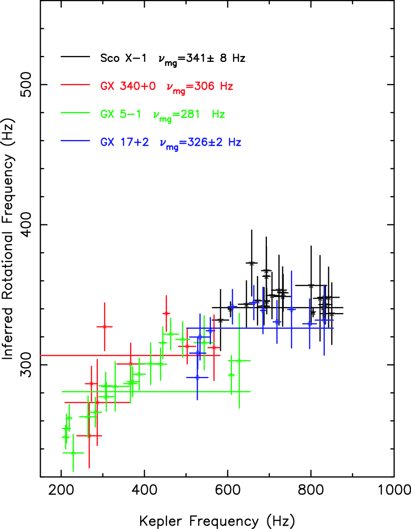
Figure 1: Inferred rotational frequencies of NS magnetosphere as a function of the Kepler frequency for a number of Z sources: Sco X-1 (black), GX 340+0 (red), GX 5-1 (green), GX 17+2 (blue). Constant rotational frequencies (possibly NS spin) for Sco X-1 and GX 17+2 (solid line) are consistent with the data. The magnetospheric rotational profiles for GX 340+0 (red), GX 5-1 is inconsistent with constant. The mean values of the rotational frequencies for these sources are given without error bars.

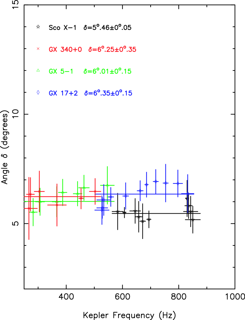
Figure 2: Inferred angles $\delta$ between rotational configuration above the disk (possibly NS magnetosphere) and the normal to the plane of Keplerian oscillations as a function of the Kepler frequency for Z-sources: Sco X-1 (black), GX 340+0 (red), GX 5-1 (green), GX 17+2 (blue). Constant $\delta-$ value is consistent with the data. The $\delta-$angle (eq.[8]) is calculated using the lower and higher kHz peaks $\nu_{1}$, $\nu_{2}$ and HBO frequencies $\nu_{HBO}$ (see text).

References

- Abramowicz et al. (2002) Abramowicz, M.A., Bulik, T., Bursa, M. & Kluz̀niak, W. 2002, A&A, in press
- Abramowicz & Kluz̀niak (2001) Abramowicz, M.A., & Kluz̀niak, W. 2001, A&A, 374, L19
- Bradshaw et al. (2002) Bradshaw, C.F., Geldzahler, B.J. & Fomalont, E.B. 2002, ApJ, submitted
- Chandrasekhar (1961) Chandrasekhar, S. 1961, Hydrodynamics and hydromagnetic stability, Oxford: Oxford at the Caredon Press
- Ford & van der Klis (1998) Ford, E., & van der Klis, M. 1998, ApJ, 506, L39
- Hide (1956) Hide, R. 1956, Quart. J. Math. Appl. Math. 9, 35
- Homan et al. (2002) Homan, J., et al. 2002, ApJ, in press (astro-ph/0104323)
- Jonker et al. (2002) Jonker, P.J., et al. 2002, MNRAS, 333, 665
- Jonker et al. (2000a) Jonker, P.J., et al. 2000a, ApJ, 537, 374
- Jonker et al. (2000b) Jonker, M., Mendez, M., & van der Klis, M. 2000b, ApJ, 540, 1049
- Lamb & Miller (2001) Lamb, F.K., Miller, M. C. 2001, ApJ, 554, 1210
- Landau & Lifshitz (1965) Landau, L.D. & Lifshitz, E.M. 1965, Mechanics, New York: Pergamon Press (LL)
- Mihalas (1970) Mihalas, D. 1970, Stellar Atmospheres, San Francisco, Calif.: W.H. Freeman 1970
- Mauche (2002) Mauche, C. W. 2002, ApJ in press (astro-ph/0207508)
- Miller et al. (1998) Miller, M.C., Lamb, F.K., Psaltis, D. 1998, ApJ 508, 791
- Osherovich & Titarchuk (1999) Osherovich, V., & Titarchuk, L. 1999, ApJ, 522, L113 (OT99)
- Psaltis et al. (1999) Psaltis, D., Belloni, & van der Klis, M. 1999, ApJ, 520, 262
- Remillard et al. (2002) Remillard, R. 2002, astro-ph/0202305
- Stella et al. (1999) Stella, G., Vietri, M., & Morsink, S.M. 1999, ApJ, 524, L66
- Strohmayer et al. (1996) Strohmayer, T.E., et al. 1996, ApJ, 469, L9
- Titarchuk (2002) Titarchuk, L.G. 2002, ApJLetters submitted
- Titarchuk, Cui & Wood (2002) Titarchuk, L.G., Cui, W. & Wood, K. 2002, ApJ, 576, L49
- Titarchuk, Lapidus & Muslimov (1998) Titarchuk, L.G., Lapidus, I.I. & Muslimov, A. 1998, ApJ, 499, 315 (TLM98)
- Titarchuk, & Osherovich (2001) Titarchuk, L., & Osherovich, V. 2001, ApJ, 555, L55
- van der Klis (2000) van der Klis, M. 2000, ARA&A, 38, 717
- van der Klis et al. (1997) van der Klis, et al. 1997, ApJ, 481, L97
- van der Klis et al. (1996) van der Klis, et al. 1996, ApJ, 469, L1
- van Straaten et al. (2002) van Straaten, S., Ford, E., van der Klis, M. & Belloni, T. 2002, ApJ, 568, 912
- van Straaten et al. (2000) van Straaten, S., Ford, E., van der Klis, M., Mendez, M. & Kaaret, Ph. 2000, ApJ, 540, 1049
- Zhang et al. (1997) Zhang, W., Lapidus, I.I., Swank J.H., White, N.E. & Titarchuk, L.G. 1997, IAU Circ, 6541