The influence of Hall drift on the magnetic fields of neutron stars

Abstract

We consider the evolution of magnetic fields under the influence of Hall drift and Ohmic decay. The governing equation is solved numerically, in a spherical shell with $r_{i}/r_{o}=0.75$. Starting with simple free decay modes as initial conditions, we then consider the subsequent evolution. The Hall effect induces so-called helicoidal oscillations, in which energy is redistributed among the different modes. We find that the amplitude of these oscillations can be quite substantial, with some of the higher harmonics becoming comparable to the original field. Nevertheless, this transfer of energy to the higher harmonics is not sufficient to significantly accelerate the decay of the original field, at least not at the $R_{B}=O(100)$ parameter values accessible to us, where this Hall parameter $R_{B}$ measures the ratio of the Ohmic timescale to the Hall timescale. We do find clear evidence though of increasingly fine structures developing for increasingly large $R_{B}$, suggesting that perhaps this Hall-induced cascade to ever shorter lengthscales is eventually sufficiently vigorous to enhance the decay of the original field. Finally, the implications for the evolution of neutron star magnetic fields are discussed.

1 Introduction

Neutron stars have the strongest magnetic fields found in the universe, with fields perhaps as large as $10^{15}$ G for so-called magnetars (e.g. Murakami 1999), around $10^{12}$ G for young ($\sim 10^{7}$ year) radio and X-ray pulsars, and a still appreciable $10^{8}-10^{10}$ G for much older ($\sim 10^{10}$ year) millisecond pulsars (e.g. Chanmugam 1992; Bhattacharya 1995; Lyne 2000). This correlation between field strength and age suggests that these very different strengths are due to the field decaying in time, rather than to any intrinsic differences between different neutron stars. One would therefore like to identify the processes causing the field to decay.

The additional observation that most weakly magnetic neutron stars have binary companions, whereas very few strongly magnetic ones do (e.g. Bhattacharya 1995), suggests that accretion of mass from the companion is somehow causing the field to decay (by mechanisms that need not concern us here, but see for example Blondin & Freese 1986; Romani 1990; Urpin & Geppert 1995). The observational evidence is unfortunately inconclusive, with Taam & van den Heuvel (1986) claiming a correlation between field strength and accreted mass, but Wijers (1997) disputing this.

One would therefore like to consider the possibility of other mechanisms besides accretion. One such alternative is Hall drift, first proposed by Jones (1988), in which the magnetic field influences itself through a quadratic nonlinearity. If it is relevant at all, Hall drift will therefore be most important for the very strongest fields – which as we saw tend to occur in isolated neutron stars, where accretion is not acting at all. Hall drift is thus likely to be the dominant mechanism influencing the magnetic fields of these stars. Of course, it could potentially be important in binaries as well, at least in the early stages while their fields are still relatively strong.

Again as a result of this quadratic nonlinearity, the timescale on which Hall drift might be expected to act is almost necessarily inversely proportional to $|{\bf B}|$. Jones suggests that it is given by

$$t_{Hall}\sim{10^{8}\over B_{12}}\;{\rm years},$$ (1)

where $B_{12}$ is the field strength in units of $10^{12}$ G. See also Goldreich & Reisenegger (1992), who obtain a similar estimate. For these $O(10^{12})$ G radio pulsars, one therefore expects a timescale comparable to their age. And indeed, Lyne, Manchester & Taylor (1985) and Narayan & Ostriker (1990) have suggested that the fields of these young pulsars do decay on a $10^{7}$ year timescale (although this too is in dispute, see for example Hartman et al. 1997; Regimbau & Pacheco 2001). Apart from the strength of the observational evidence though, the mere fact that Hall drift could affect the fields of neutron stars on timescales so short compared to their evolutionary timescales makes it worthy of study.

There is one slight difficulty though in attributing this possible $10^{7}$ year decay rate to Hall drift, namely that the Hall effect conserves magnetic energy, and therefore by itself cannot cause any field decay at all. The suggestion therefore is that the Hall term, being nonlinear, will redistribute energy among the different modes, and in particular will initiate a cascade to ever shorter lengthscales, where ordinary Ohmic decay (which only acts on $O(10^{10})$ year timescales at the longer lengthscales) can destroy the field.

Since this mechanism was first proposed by Goldreich & Reisenegger, detailed calculations have been done by a number of authors, including Naito & Kojima (1994), Muslimov (1994), Muslimov, Van Horn & Wood (1995), Shalybkov & Urpin (1997) and Urpin & Shalybkov (1999). Of these, only the last two were in the astrophysically relevant limit of large Hall parameter $R_{B}$ though, where $R_{B}$ measures the ratio of the Ohmic timescale to the Hall timescale, and is defined more precisely below. However, it is not certain whether their results were fully resolved, as they had only 20 radial by 40 latitudinal finite difference points.

In contrast, we have 25 radial by 100 latitudinal spectral expansion functions, and obtain fully resolved solutions for $R_{B}$ up to $O(100)$ (comparable to what Shalybkov & Urpin achieved, and indeed in broad agreement with their results, suggesting that perhaps their resolution was good enough after all to resolve the most important features anyway). Even at these large values, however, we find that while the Hall effect does indeed induce a significant redistribution of energy among the different modes, it does not appear to be enough to cause the lowest modes to decay substantially faster than they would have otherwise.

Before applying this conclusion to real neutron stars though, it is important to qualify it by noting that our calculations (as well as the others cited above) are restricted to $\bf B$ being axisymmetric, and the various material properties such as the density being independent of depth. Neither of these assumptions holds in real neutron stars, and relaxing either could significantly alter the results. For example, Vainshtein, Chitre & Olinto (2000) show that including variations in density introduces new effects even for field configurations where no ordinary Hall drift would be present at all. Similarly, Rheinhardt & Geppert (2002) also consider field configurations where no ordinary Hall cascade is present, but claim that instabilities, including non-axisymmetric ones, can nevertheless arise. We will discuss both of these papers more fully below, as well as how these two restrictions might be relaxed in future work.

2 Equations, etc.

2.1 The Evolution Equation for $\bf B$

The equation governing the evolution of a magnetic field under the influence of Hall drift and Ohmic decay is

$${\partial{\bf B}\over\partial t}=-\nabla\times\Bigl{(}{c\over 4\pi ne}\,{(\bf\nabla\times B)\times B}\Bigr{)}$$

$$\phantom{{\partial{\bf B}\over\partial t}=}-\nabla\times\Bigl{(}{c^{2}\over 4\pi\sigma}\,\nabla\times{\bf B}\Bigr{)},$$ (2)

where $n$ is the electron number density, $\sigma$ the conductivity, $e$ the electron charge and $c$ the speed of light. See for example Goldreich & Reisenegger (1992) for the details of the derivation. We then nondimensionalize according to

$${\bf B}=B_{0}\,{\bf B^{*}},\qquad l=r_{o}\,l^{*},\qquad t=\tau\,t^{*},$$ (3)

where $B_{0}$ is a typical field strength, $r_{o}$ the radius of the star, and

$$\tau={4\pi ner_{o}^{2}\over cB_{0}}$$ (4)

the Hall timescale, where we note, incidentally, that these estimates (1) amount to nothing more than inserting particular numbers into this result (4) obtained purely by dimensional analysis. We also note, though, that while we’ve implicitly assumed $n$ to be constant here, in real neutron stars it varies by several orders of magnitude throughout the depth of the crust. It is therefore somewhat misleading to talk about a single Hall timescale; there is rather a range of timescales, from perhaps $10^{5}/B_{12}$ up to $10^{8}/B_{12}$ years.

Dropping the asterisks again, we obtain

$${\partial{\bf B}\over\partial t}=-\nabla\times\bigl{(}{(\bf\nabla\times B)\times B}\bigr{)}+R_{B}^{-1}\,\nabla^{2}{\bf B},$$ (5)

where we’ve assumed $\sigma$ to be constant as well (again not the case in real neutron stars). The Hall parameter

$$R_{B}={\sigma B_{0}\over nec},$$ (6)

and is up to $10^{2}$ to $10^{3}$ in the crusts of $O(10^{12})$ G neutron stars, where we will apply (5). One useful physical interpretation to associate with $R_{B}$ is the ratio of the Ohmic timescale $4\pi\sigma r_{o}^{2}/c^{2}$ to this Hall timescale $\tau$.

2.2 Cascades?

We note that this Hall equation (5) bears certain similarities to the vorticity equation of ordinary fluid dynamics,

$${\partial{\bf\Omega}\over\partial t}=\nabla\times\bigl{(}{\bf U\times\Omega}\bigr{)}+Re^{-1}\,\nabla^{2}{\bf\Omega},$$ (7)

where $\bf U$ and $\bf\Omega=\nabla\times U$ are the velocity and vorticity, respectively, and $Re$ the Reynolds number. It is on the basis of these similarities that Goldreich & Reisenegger suggested that the Hall effect would initiate a cascade to ever shorter wavelengths, analogous to the Kolmogorov cascade in ordinary fluid turbulence. By applying arguments from turbulence theory, they went on to suggest that the power spectrum of Hall turbulence should fall off like $k^{-2}$, where $k$ is the wavenumber, and that the dissipation scale should be reached when $k=O(R_{B})$.

However, there is also one crucial difference between (5) and (7), one that we believe has perhaps not been sufficiently appreciated before. In particular, in (7) the nonlinear term contains only first derivatives of $\bf\Omega$, whereas in (5) the nonlinear term contains second derivatives of $\bf B$. This has at least two important consequences.

First, in (5) the coefficients of the second derivative terms then depend on the solution itself, whereas in (7) they don’t. This raises the possibility that the mathematical character of the Hall equation could switch, from parabolic to hyperbolic. What would happen then is not clear, but the effect could be dramatic, given how different these two types of equations are. See, for example, Ockendon et al. (1999) for the theory behind the classification of partial differential equations into parabolic, hyperbolic, or elliptic types, depending on the sign of certain combinations of the coefficients of the second derivative terms.

Second, in (7) one can always be certain that if one just goes to sufficiently short lengthscales, the diffusive term will eventually dominate the advective term, regardless of how large $Re$ is. In contrast, in (5) one can go to arbitrarily short lengthscales, and still not be certain that the diffusive term will dominate the Hall term, because they both scale quadratically with the wavenumber. That means though that the whole notion of a definite dissipation scale is much less clear in (5) than in (7). One obtains a definite dissipation scale only if one simply assumes that the coupling is purely local in wavenumber space. The argument is essentially as follows:

By definition, the dissipation scale occurs when the local Hall parameter is $O(1)$. What is the ‘local’ Hall parameter though, when the defining equation (6) doesn’t involve lengthscales at all?? Well, if the coupling is purely local in wavenumber space, then implicitly (6) does involve lengthscales after all, since then the $B_{0}$ that should be used is the field at that wavenumber only, rather than the total field. That is, one has

$$R_{B}^{\prime}=R_{B}\cdot(B^{\prime}/B),$$ (8)

where the primed quantities denote these small-scale, local values, and the unprimed the large-scale, global. If in addition one has a $k^{-2}$ power spectrum, then $B^{\prime}/B\sim k^{-1}$, so $R_{B}^{\prime}$ is indeed reduced to $O(1)$ when $k=O(R_{B})$. We can see though how crucially the argument depends on the coupling being purely local in wavenumber space; if this does not hold then $R_{B}^{\prime}=R_{B}$, and one simply does not obtain a definite dissipation scale at all. (We note also that there is no reason why the spectrum should not just drop off like $k^{-p}$ indefinitely; provided $p>1$ the total energy would certainly still be bounded.)

2.3 Instabilities?

Another intriguing idea, intended precisely to explore this issue of whether the coupling is purely local in wavenumber space, is due to Rheinhardt & Geppert (2002), who considered fields satisfying

$$\nabla\times\bigl{(}{(\bf\nabla\times B)\times B}\bigr{)}=0,$$ (9)

so that no ordinary Hall cascade is present. Linearizing (5) about such a basic state, one obtains

$${\partial{\bf b}\over\partial t}=-\nabla\times\bigl{(}{(\nabla\times{\bf b})\times{\bf B}_{0}}+{(\nabla\times{\bf B}_{0})\times{\bf b}}\bigr{)}$$

$$\phantom{{\partial{\bf b}\over\partial t}=}+R_{B}^{-1}\,\nabla^{2}{\bf b}.$$ (10)

Neglecting the Ohmic decay of the basic state ${\bf B}_{0}$, one therefore has a simple eigenvalue problem for the growth or decay rates of the perturbations $\bf b$. Rheinhardt & Geppert then found that for sufficiently large $R_{B}$ arbitrarily short lengthscales could still be excited, which, they claimed, proves that the coupling is not purely local in wavenumber space.

The difficulty we have with this approach is that while these small scale modes may indeed be excited, we do not believe they can be distinguished from the action of the ordinary Hall cascade. In particular, while these small scale modes do grow, the fastest growing modes are always large scale. As soon as these are excited though, the field no longer satisfies (9), and will therefore generate an ordinary cascade, which is likely to reach these small scales well before these postulated instabilities become significant. For example, our integration times here are sufficiently short that these instabilities should not be manifesting themselves, and yet we do obtain very short lengthscales, suggesting that it is the cascade rather than the instabilities that is most significant. Indeed, once the cascade is established, it makes little sense at all to consider the growth or decay rates of isolated modes. The problem is intrinsically nonlinear, and must be solved as such.

Finally, one might just note that there is one type of instability that could be unambiguously distinguished from the ordinary cascade, namely a non-axisymmetric one. Here we will consider only axisymmetric solutions, so the issue does not arise, but in general one might ask how one could go from two-dimensional to three-dimensional solutions. In particular, if one starts with a 2D field, the ordinary cascade will forever remain 2D as well. The only way to obtain a 3D field is via an instability to a non-axisymmetric mode. Of course, as soon as one does have a 3D field, the cascade will also be 3D, so one would again find it difficult to distinguish between the cascade and the instability. The initial trigger though that allows the field, and hence also the cascade, to go from 2D to 3D would clearly have to be a non-axisymmetric instability of some sort.

2.4 T-P Decomposition

Returning to our development of (5), for these axisymmetric fields we will consider here, it is convenient to decompose $\bf B$ into toroidal and poloidal components

$${\bf B}={\bf B}_{t}+{\bf B}_{p}=B{\bf\hat{e}}_{\phi}+\nabla\times(A{\bf\hat{e}}_{\phi}).$$ (11)

Equation (5) then yields

$${\partial A\over\partial t}=-{\bf\hat{e}}_{\phi}\cdot\bigl{(}(\nabla\times{\bf B}_{t})\times{\bf B}_{p}\bigr{)}+R_{B}^{-1}D^{2}A,$$ (12)

$${\partial B\over\partial t}=-{\bf\hat{e}}_{\phi}\cdot\nabla\times\bigl{(}(\nabla\times{\bf B}_{p})\times{\bf B}_{p}+(\nabla\times{\bf B}_{t})\times{\bf B}_{t}\bigr{)}$$

$$\phantom{BB=\,}+R_{B}^{-1}D^{2}B,$$ (13)

where

$$D^{2}f={1\over r}{\partial^{2}\over\partial r^{2}}\Bigl{(}fr\Bigr{)}+{1\over r^{2}}{\partial\over\partial\theta}\Bigl{(}{1\over\sin\theta}{\partial\over\partial\theta}\bigl{(}f\sin\theta\bigr{)}\Bigr{)}.$$ (14)

We note then that if the field is initially purely toroidal it will remain so, whereas if it is initially purely poloidal it will immediately induce a toroidal part as well, and once both components are present each will act back on the other.

2.5 Boundary Conditions

Taking the region exterior to the star to be a source-free vacuum, the outer boundary conditions are simply

$$B=0,\qquad\Bigl{(}{d\over dr}+{l+1\over r}\Bigr{)}\,A=0\qquad{\rm at\ }r=r_{o},$$ (15)

where $l$ is the spherical harmonic degree. Since the numerical solution already involves decomposition of $A$ and $B$ into Legendre functions, implementing this $l$-dependent boundary condition presents no difficulties.

The inner boundary conditions are not quite so straightforward, and depend very much on what assumptions we make about the interior of the star, about which little is known for certain. However, one common assumption (e.g. Bhattacharya & Datta 1996; Konenkov & Geppert 2001) is that it is superconducting, in which case the magnetic field will be expelled from it. The boundary conditions are then that the normal component of the magnetic field and the tangential components of the associated electric field must vanish. $B_{r}=0$ immediately yields $A=0$, but $E_{t}=0$ is a little more complicated, and requires a little algebra before yielding

$${1\over r\sin\theta}{\partial\over\partial\theta}\Bigl{(}B\sin\theta\Bigr{)}B+R_{B}^{-1}\,{1\over r}{\partial\over\partial r}\Bigl{(}Br\Bigr{)}=0.$$ (16)

Such a nonlinear boundary condition is unfortunately very difficult to implement. We would therefore like to simplify it in some way. We do so by noting that in the relevant $R_{B}\gg 1$ limit the second term ought to be negligible (assuming $\partial B/\partial r$ does not increase with $R_{B}$, that is, assuming that no boundary layers develop), in which case we are left with just $B=0$. For our inner boundary conditions we therefore take

$$B=0,\qquad A=0\qquad{\rm at\ }r=r_{i}.$$ (17)

The radii at which we will apply these boundary conditions are $r_{i}=0.75$ and $r_{o}=1$. Although this is still not quite as thin as neutron star crusts are believed to be ($r_{i}/r_{o}\approx 0.9$ would be more appropriate), it should be enough to capture most of the geometrical effects of having a thin shell, but without experiencing numerical difficulties due to too extreme a disparity between the radial and latitudinal lengthscales.

Finally, a few runs were also done with insulating boundaries inside as well as outside. This is obviously not realistic, but allows one to assess the extent to which the solutions are affected by differing boundary conditions. It turned out that while this certainly altered the quantitative details, the general features remained the same.

2.6 Initial Conditions

In many problems the specific initial conditions are largely irrelevant, as one is only interested in the final, equilibrated solutions. In this case though, the only ‘equilibrated’ solution is ${\bf B}=0$, since (as noted above, and as we will show below), all solutions of (5) necessarily decay in time. So, what we are interested in instead is to start with some particular initial condition, and study the precise manner of the decay, whether it is significantly faster than just Ohmic decay, whether higher harmonics are excited in the process, etc. In this problem therefore we need to give careful consideration to our choice of initial conditions.

If we temporarily neglect the Hall terms in equations (12) and (13), we can solve for the individual free decay modes. Figure 1 shows the lowest $l=1$ and $l=2$ poloidal modes, and also the lowest $l=2$ toroidal mode. The free decay rates for these three modes are $49R_{B}^{-1}$, $61R_{B}^{-1}$, and $166R_{B}^{-1}$. We label them ${\bf B}_{p1}$, ${\bf B}_{p2}$, and ${\bf B}_{t2}$, and normalize them so that $B_{r}(r_{o},0)=1$ for the poloidal modes, and $B_{\rm max}=1$ for the toroidal mode. Our initial conditions will then consist of either these modes in isolation, or else simple linear combinations of them.

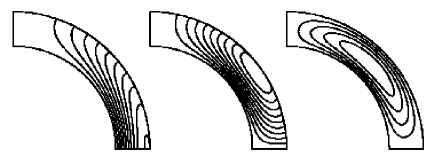
Figure 1: Field lines of the two poloidal modes ${\bf B}_{p1}$ and ${\bf B}_{p2}$, and contours of the toroidal mode ${\bf B}_{t2}$. ${\bf B}_{p1}$ is equatorially symmetric, ${\bf B}_{p2}$ and ${\bf B}_{t2}$ antisymmetric.

2.7 Symmetries

At this point it is worthwhile also to briefly consider some of the symmetries associated with (12) and (13), to avoid doing effectively duplicate runs. For example, (5) is clearly not invariant under ${\bf B}\rightarrow-{\bf B}$, so do we need to consider $\pm{\bf B}_{p1}$, $\pm{\bf B}_{p2}$, and $\pm{\bf B}_{t2}$ separately? Well, $\pm{\bf B}_{p1}$ are physically the same, just turned upside down, so clearly not in that case. For $\pm{\bf B}_{p2}$ though it’s not so obvious, since these are not the same; $+{\bf B}_{p2}$ has the field inward in a ring around the equator, and outward at the poles, whereas $-{\bf B}_{p2}$ has the reverse, and no amount of tilting or turning will cause the two to coincide. Nevertheless, one can see easily enough that $\pm{\bf B}_{p2}$ will still evolve in exactly the same way, by noting that (12) is linear in $A$, whereas (13) contains only even powers of $A$. Reversing the sign of any initial poloidal field will therefore always yield exactly the same evolution. Then, having noted how $A$ enters into (12) and (13), and how that affects this $\pm$ symmetry, it is an easy matter to verify that because $B$ enters differently, it does not share this symmetry. In general, therefore, reversing the sign of an initial toroidal field will affect the evolution. We will therefore have to consider $\pm{\bf B}_{t2}$ separately.

Another symmetry worth mentioning is the equatorial symmetry, particularly as this is somewhat different from that usually encountered in stellar dynamos. One may readily verify that solutions exist having $A$ either symmetric or antisymmetric, but with $B$ antisymmetric in both cases. In contrast, in stellar dynamo models the parity of $B$ would also change, always being the opposite of $A$’s (e.g. Knobloch, Tobias & Weiss 1998). We can see easily enough though that that cannot be the case here, by noting this same property of (12) and (13) already used above, that $A$ enters linearly in (12), and as even powers only in (13). Therefore, if either pure parity is allowed for $A$ at all, the opposite one must also be allowed, but with $B$ having the same parity in both cases. Being aware of these equatorial symmetries is obviously helpful as well in doing the runs, as one can then reduce the computational effort by a factor of two for many of them.

Finally, combining the plus/minus and equatorial symmetries, we note in passing that if one has an initial poloidal field that is equatorially asymmetric, one may reverse the sign of either the symmetric or the antisymmetric parts separately, and will still obtain exactly the same evolution, with the only effect on the toroidal field being to reverse the sign of its symmetric part (which is consistent, of course, with this part being absent if $A$ has a pure parity, and also consistent with $B$ being unchanged if both parts of $A$ are reversed).

2.8 Numerical Solution

The code we use to solve (12), (13), (15) and (17) is a suitably modified version of the spherical harmonic code described by Hollerbach (2000), where we include modes up to $l=100$, and 25 Chebychev polynomials in the radial direction. A few runs were also redone at truncations as low as $70\times 20$, and as high as $120\times 30$, to check whether $100\times 25$ is adequate. We believe that the solutions presented here are indeed fully resolved, although one of them does show some unusual features in its power spectrum, as we will discuss below.

We note also that at $100\times 25$, we are capable of resolving structures as fine as $r_{o}\Delta\theta=\pi/100=0.03$ in latitude, and $\Delta r=0.25/25=0.01$ in radius (strictly speaking probably only structures two or three times greater in each case, to allow for the fact that two or three collocation points are needed to resolve a given ‘structure’). Even though the truncation in $r$ is lower, the resolution is therefore already higher. The reason for this is that in such a thin shell one might also expect finer structures to develop in $r$, as will indeed turn out to be the case (although typically not three times finer).

Finally, the timestep used was $\Delta t=10^{-7}$ for most runs, with again a few done at even smaller values. Such small values were necessary to avoid numerical instabilities. The origin of these instabilities is almost certainly the previously noted feature that the Hall term (which is treated explicitly) contains just as many derivatives as the Ohmic term (treated implicitly). It is certainly well known that treating second derivative terms explicitly almost invariably requires extremely small timesteps, with the maximum allowable $\Delta t$ also decreasing very quickly with increasing truncation, as was found to be the case here.

Once again, also, this feature that the Hall term has just as many derivatives as the Ohmic term raises the possibility that the governing equation (5) could switch from parabolic to hyperbolic. What would happen then is not clear, but the code certainly could not cope with that. And indeed, we will find that there are limits beyond which we simply cannot push $R_{B}$, no matter how much we reduce $\Delta t$, indicating that perhaps such a switch has occurred.

2.9 The Magnetic Energy Equation

As noted above, one major purpose of this work is to address the question as to whether the Hall effect can significantly accelerate the decay of a magnetic field despite the fact that by itself it conserves magnetic energy. It therefore seems appropriate to verify that it really does so, and in the process derive a useful diagnostic equation to help assess the accuracy of our numerical solutions. To obtain this equation for the magnetic energy, we begin by taking the dot product of (5) with $\bf B$ and applying various vector identities to obtain

$${\partial\over\partial t}{{\bf B}^{2}\over 2}=-\nabla\cdot\bigl{[}{\bf(J\times B)\times B}+R_{B}^{-1}\,({\bf J\times B})\bigr{]}$$

$$\phantom{{\partial\over\partial t}{{\bf B}^{2}\over 2}=}-R_{B}^{-1}\,{\bf J}^{2},$$ (18)

where $\bf J=\nabla\times B$. When integrated over the shell, therefore, the Hall term will contribute only surface integrals at $r_{i}$ and $r_{o}$, whereas the diffusive term will contribute both surface integrals and a negative-definite volume integral.

In order to obtain our desired result, we therefore need to consider these various surface terms very carefully, particularly the ones at $r_{i}$, where we remember our $B=0$ boundary condition is only a computationally convenient approximation to the true condition (16). If this approximation should turn out to yield some spurious source or sink of energy through the boundary, we would not be able to use it after all. We must therefore show that

$${\bf\hat{e}}_{r}\cdot\bigl{[}{\bf(J\times B)\times B}+R_{B}^{-1}\,({\bf J\times B})\bigr{]}=0\qquad{\rm at\ }r=r_{i}.$$ (19)

To do so, we begin by noting that in terms of the individual components $(B_{r},B_{\theta},B_{\phi})$ and $(J_{r},J_{\theta},J_{\phi})$,

$$A=B=0\quad\Longrightarrow\quad B_{r}=B_{\phi}=J_{r}=0,$$ (20)

so that, using also the generally valid result $J_{\phi}=-D^{2}A$,

$${\bf J\times B}=(B_{\theta}\,D^{2}A,0,0)\qquad{\rm at\ }r=r_{i}.$$ (21)

Next, (12) can be expressed as

$${\partial A\over\partial t}=J_{\theta}B_{r}-J_{r}B_{\theta}+R_{B}^{-1}D^{2}A,$$ (22)

so applied at $r_{i}$, where we remember $A=B_{r}=J_{r}=0$, we find that $D^{2}A=0$ as well. We therefore have that

$${\bf J\times B}=0\qquad{\rm at\ }r=r_{i},$$ (23)

which establishes our required result (19).

In contrast, at $r_{o}$ one finds that these surface terms do not vanish. Instead, they turn out to be precisely what is needed to take into account changes in the energy stored in the external field. The final result is then

$${\partial\over\partial t}\,{1\over 2}\int{\bf B}^{2}\,dV=-R_{B}^{-1}\int{\bf J}^{2}\,dV,$$ (24)

where the integral on the left extends over $r\geq r_{i}$, and the one on the right over $r_{i}\leq r\leq r_{o}$. Equation (24) is thus the desired energy balance, namely that the total magnetic energy in all of space decreases only as a result of Ohmic decay. Hall drift rearranges the field, and hence also the energy, but neither creates nor destroys it.

In addition to its role in illuminating the physics of Hall drift and Ohmic decay, (24) is also a very useful diagnostic tool in assessing the accuracy of our solutions. Reassuringly, we found that not only does the magnetic energy indeed decrease monotonically in time (hardly a very stringent test), but that all of our runs satisfied (24) to within 1 per cent or better. That is, if we (a posteriori) compute the quantity

$$q={\bigg{|}{\partial\over\partial t}\,{1\over 2}\int{\bf B}^{2}\,dV+R_{B}^{-1}\int{\bf J}^{2}\,dV\bigg{|}\;\bigg{/}\;R_{B}^{-1}\int{\bf J}^{2}\,dV},$$ (25)

then $q$ never exceeded 0.01, with typical values being much smaller still. For example, if we consider not the maximum values, but instead the rms values over a given run, then $q_{\rm rms}$ never exceeded 0.001.

3 Results

3.1 Initial Condition ${\bf B}_{p1}$

Following Shalybkov & Urpin (1997), we start with the simplest possible initial condition, namely just the lowest poloidal decay mode ${\bf B}_{p1}$. Figure 2 shows how the first three harmonics $b_{1}$, $b_{3}$ and $b_{5}$ of the external field then evolve in time, where these $b_{l}$ are defined by

$$B_{r}(r_{o},\theta,t)=\sum_{l}\,b_{l}(t)\,P_{l}(\cos\theta).$$ (26)

That is, $b_{l}(0)$ is nothing more than the coefficient of ${\bf B}_{pl}$ in our initial condition. And indeed, we note how $b_{1}$ starts out at 1, and then slowly decays. It does not decay monotonically, but never deviates very much from the $\exp(-49R_{B}^{-1}\,t)$ rate that Ohmic decay alone would have yielded. For these runs at least, the inclusion of Hall drift has not significantly changed the decay rate.

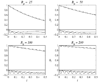
Figure 2: The harmonics $b_{1}$, $b_{3}$ and $b_{5}$ as functions of time, for the four indicated values of $R_{B}$. The solid line starting at 1 is $b_{1}$, with the dashed line being the $\exp(-49R_{B}^{-1}\,t)$ decay rate of Ohmic decay alone. The next largest solid line is $b_{3}$, and the smallest $b_{5}$.

That is not to say that Hall drift has no influence on the field though; we note how $b_{3}$ oscillates, on a timescale of approximately 0.05, and reaching amplitudes as large as 0.15, with both the period and the amplitude largely independent of $R_{B}$. Converting back to dimensional time therefore, we could expect periods on the order of

$$T\sim 0.05\times{10^{8}\over B_{12}}\;{\rm years},$$ (27)

or $O(10^{5})$ years for the very strongest fields. These so-called helicoidal oscillations are in excellent agreement with those previously obtained by Shalybkov & Urpin, who went on to derive an associated dispersion relation, verifying that one should obtain waves that oscillate on the $O(1)$ Hall timescale and decay on the $O(R_{B})$ Ohmic timescale, exactly as we see here.

Based on these results therefore, one would think that the solution ought to exist for arbitrarily large $R_{B}$, with the only effect of ever larger values being to postpone to ever larger times the decay of both the main field $b_{1}$ and these oscillations in the induced field $b_{3}$. Well, perhaps such a solution does exist for arbitrarily large $R_{B}$, but we certainly could not obtain it numerically. Every attempt to increase $R_{B}$ much beyond 200 failed, even at truncations as high as $120\times 30$ and timesteps as small as $10^{-8}$.

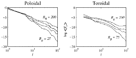
Figure 3: Log$<\!\!E_{l}\!\!>$ versus $\log l$, where the $<>$ brackets indicate an average over $t$ between 0.4 and 0.5 – long enough to average over these helicoidal oscillations, but short enough to be largely unaffected by the overall decay. The (barely visible) dotted lines show $R_{B}=100$ at truncation $70\times 20$.

We can perhaps begin to understand why by considering the power spectra shown in figure 3. Here

$$E_{l}={1\over 2}\int{\bf B}_{l}^{2}\,dV$$ (28)

is the energy contained in the $l$-th spherical harmonic mode, either poloidal or toroidal, and as in (24) the integration over $r$ includes the energy in the exterior vacuum field. (And of course the cross-terms $\int{\bf B}_{l_{1}}\cdot{\bf B}_{l_{2}}\,dV$ vanish by the orthogonality of the spherical harmonics. The total energy is thus indeed just the sum of these individual $E_{l}$.)

Turning to the poloidal spectra first, we note that the $R_{B}=200$ curve follows an $l^{-5}$ scaling over the entire range of $l$, whereas the lower $R_{B}$ curves start out much the same, but then drop off somewhat more rapidly, exactly as one might expect. We note though that there is no sign of a definite dissipation scale, either at the $l=O(R_{B})$ appropriate to an $l^{-2}$ spectrum, or the $l=O(R_{B}^{2/5})$ appropriate to an $l^{-5}$ spectrum. As discussed in section 2.2, this suggests that the coupling is not purely local in wavenumber space. We note also that this particular exponent $-5$ is rather different from the $-2$ predicted by Goldreich & Reisenegger (1992), but of course one should hardly expect the two to be the same, given that their result applies to 3D turbulence, whereas our calculations here are 2D laminar.

Turning to the toroidal spectra next, for small $l$ they too are of the form $l^{p}$, but now the exponent is around $-3.5$ rather than $-5$ or $-2$. The entire curves also shift upward slightly with increasing $R_{B}$, and show no sign of saturating for sufficiently large values. Probably more worrisome though is the behaviour for large $l$, where the $R_{B}=200$ curve actually rises ever so slightly between $l=60$ and 100. However, runs done at truncations varying between 80 and 120 all showed this same minimum at $l=60$, suggesting that it is real, and not some numerical artifact. Furthermore, the $R_{B}=100$ and 50 curves also show slight rises but still fall again thereafter, so perhaps the $R_{B}=200$ curve would too, if only we could include enough modes. It is nevertheless not quite clear what to make of this $R_{B}=200$ curve, and whether it really is fully resolved at the truncations we can afford. Based on these spectra though, we can certainly understand why attempting to increase $R_{B}$ further still was not successful.

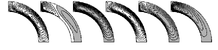
Figure 4: Contour plots of the $R_{B}=200$ toroidal field at times 0.4, 0.42, $\ldots$, 0.5, with a contour interval of 0.01, and negative regions grey-shaded. The poloidal field is not shown, as it is essentially unchanged from ${\bf B}_{p1}$ (which is only to be expected if $b_{3}$ never exceeds 0.15).

Briefly returning also to the results of Shalybkov & Urpin, we have already noted that they too obtained helicoidal oscillations much like those in figure 2. Unfortunately, they did not plot power spectra at all, but simply stated that only the $l\leq 5$ modes “give an appreciable contribution,” without further comment on what that means quantitatively. With 40 latitudinal finite difference points they were actually resolving considerably more than just the $l\leq 5$ modes though – although of course considerably less than the 100 modes we have resolved here. It is nevertheless surprising that they obtained such good results with such a low resolution. (In contrast, the fact that they worked in a full sphere rather than a thin shell makes very little difference; we also did a few runs with $r_{i}/r_{o}=0.5$ and 0.25, and obtained spectra quite similar to those in figure 3.)

Finally, we would like to know what the solutions actually look like, and in particular see whether we can identify the features corresponding to these ever flatter spectra. Figure 4 shows the field for $R_{B}=200$ and $t$ between 0.4 and 0.5, that is, covering the last two of these helicoidal oscillations in figure 2 (and also precisely the time over which the spectra in figure 3 were averaged). We see that these oscillations involve reversals in the sign of $B$, originating at the equator and propagating to the poles. What we do not see, however, are any small scale features corresponding to this part of the spectrum between 60 and 100. In retrospect this is probably not surprising though, since this plateau is after all 6 orders of magnitude down from the large scale features, and therefore shouldn’t be expected to be visible on a simple contour plot such as this. In some of our solutions below though we will see small scale features as well, at which point we will better understand why they break down for sufficiently large $R_{B}$.

3.2 Initial Conditions ${\bf B}_{p1}+a\,{\bf B}_{t2}$

The maximum toroidal field in figure 4 is only 0.1, and even in the earlier stages of evolution it never exceeds 0.25. It is therefore probably not surprising that $b_{3}$ never becomes comparable with $b_{1}$, since according to (12) the toroidal field is a crucial ingredient in inducing higher harmonics in the poloidal field. If we did have a larger toroidal field though, it seems likely we would also obtain a larger $b_{3}$, perhaps even comparable with $b_{1}$. To test this hypothesis, we add some constant $a$ times ${\bf B}_{t2}$ to our previous initial condition ${\bf B}_{p1}$. This choice is also consistent with the well-known fact that most dynamo models generate toroidal fields at least as strong, if not stronger, than the poloidal field. If we’re assuming that our initial condition was generated by some previously acting dynamo, it therefore seems reasonable to take an initial toroidal field at least as strong as our initial poloidal field, that is, $|a|\geq 1$ (and from section 2.7 we remember that here we will indeed have to consider $\pm a$ separately).

Figure 5 shows the results for $|a|=1$ and $R_{B}=25$ and 50. We obtain the same helicoidal oscillations as before, on much the same $\sim 0.05$ timescale as before. Now, however, the maximum amplitude of $b_{3}$ is indeed greater, around 0.2 for $a=1$ and 0.3 for $a=-1$. Except for such minor quantitative details, the only other effect of reversing the sign of $a$ though is to reverse the initial deflection of $b_{3}$ (and of $b_{1}$ as well). And again as before, the only effect of increasing $R_{B}$ that is evident here is to delay the inevitable decay of both the main field and the induced oscillations.

Figure 6 shows the results for $|a|=2$, $R_{B}=50$, and for $|a|=3$, $R_{B}=25$. And not surprisingly, the maximum amplitude of $b_{3}$ is greater still, almost 0.5 for $|a|=2$, 0.62 for $a=-3$, and 0.76 for $a=3$. Based on these results, therefore, it seems that one should be able to make the maximum amplitude of $b_{3}$ arbitrarily large, simply by taking $a$ sufficiently large. As before though, all attempts to increase $a$ (and/or $R_{B}$) much beyond the values in figure 6 failed, no matter how small a timestep was tried. And not surprisingly, the reason for this failure is also much as before. Figure 7 shows power spectra for $R_{B}=25$ and $a=1$, 2, 3, and we note that increasing $a$ also causes the spectra to become flatter and flatter, until by $a=3$ the poloidal spectrum falls off by only 7 orders of magnitude, and the toroidal by 6.

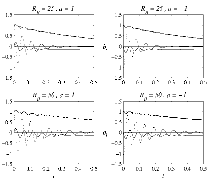
Figure 5: As in figure 2, the solid line starting at 1 is $b_{1}$ as a function of $t$, with the dashed line again being the $\exp(-49R_{B}^{-1}\,t)$ decay rate of Ohmic decay alone. The solid line starting at 0 is again $b_{3}$. The dotted line starting at $\pm 1$ is the toroidal field at $r=0.875$, $\theta=\pi/4$, where ${\bf B}_{t2}$ takes its maximum value.

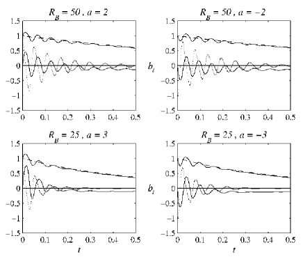
Figure 6: As in figure 5, except that now the dotted line is $B(0.875,\pi/4)/|a|$. We see therefore that increasing $a$ simply scales up the toroidal field, but otherwise has virtually no effect on it, only on $b_{3}$.

The toroidal spectrum therefore drops off by 6 orders of magnitude for both the $R_{B}=200$ run above, as well as for this $a=3$ run here. Here though the dropoff is much more uniform between $l=2$ and 100, whereas above we remember it all occurred between 2 and 60. That necessarily means then that this run has more power in the intermediate range. If we are therefore trying to identify the features corresponding to these ever flatter spectra, this is the run to consider. Figure 8 shows the field up to $t=0.06$, so the first of these oscillations this time. We note how they again involve reversals in the sign of $B$. This time, however, we can also see some small scale structures emerging; at $t=0.025$ and again between 0.05 and 0.06 some of the contour lines near the equator crowd very close together, indicating the formation of very intense currents. (Some of the contour lines near the inner boundary also crowd very close together, suggesting that our $B=0$ boundary condition – which we remember depended on $\partial B/\partial r$ being small – should be viewed as a mathematically convenient toy model rather than a physically accurate approximation.)

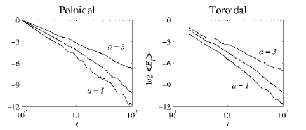
Figure 7: Power spectra of the solutions for $R_{B}=25$ and $a=1$, 2 and 3, this time averaged between $t=0$ and 0.1 to avoid the subsequent very strong decay. As one might expect, the spectra for $R_{B}=50$, $a=1$ and 2, are flatter than the corresponding ones for $R_{B}=25$, but still not as flat as the $a=3$ ones shown here. We therefore show only the $R_{B}=25$ spectra, to focus attention on the variation with $a$. We also note how all of these spectra are roughly of the form $l^{p}$, with $p$ varying between $-3.5$ and $-6$ for both poloidal and toroidal.

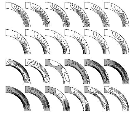
Figure 8: The structure of the $R_{B}=25$, $a=3$ field, at times 0.005, 0.01, $\ldots$, 0.06. The top two rows show the poloidal field, where we note that now we do see significant departures from ${\bf B}_{p1}$, namely the emergence of field lines closing entirely in one hemisphere. The bottom two rows show the toroidal field, with a contour interval of 0.25, and negative regions again grey-shaded.

So here we have the small scale structures corresponding to the ever flatter spectra, and therefore also the reason we cannot increase $R_{B}$ and/or $a$ indefinitely. As we increase these parameters, these structures get finer and finer, until we can no longer resolve them, and the code inevitably crashes. The only remaining questions then are precisely how the thickness of these structures scales with $R_{B}$, and whether the governing equations always remain parabolic, or whether some critical $R_{B}$ is eventually reached beyond which they switch to hyperbolic at various points in space and time. What would happen after that is completely unknown, of course, and unfortunately not answerable with this code.

3.3 Initial Condition ${\bf B}_{p2}$

Figure 9 shows the results starting with ${\bf B}_{p2}$ as the initial condition. Comparing with figure 2, we see that one obtains far larger oscillations in the higher harmonics, with even $b_{8}$ still attaining a quite substantial amplitude. The period is also longer, 0.2 instead of 0.05. As before though, both the period and the amplitude are only weakly dependent on $R_{B}$, and even that probably only because here we cannot achieve sufficiently high values to have much more than one cycle before everything decays. And we note, incidentally, that now the main field $b_{2}$ does decay slightly faster than Ohmic decay alone would have dictated, but still not enough to be significant. Finally, figure 10 shows the field through the first of these oscillations, and again we see the emergence of very small scale structures at certain times.

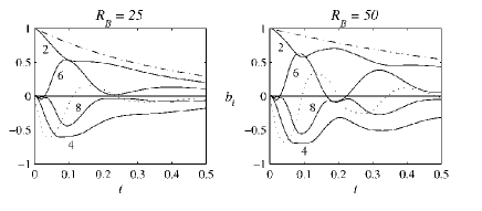
Figure 9: The harmonics $b_{2}$ through $b_{8}$ as functions of time. The dashed line is now the $\exp(-61R_{B}^{-1}\,t)$ decay rate of $b_{2}$ if Ohmic decay alone were acting. Finally, the dotted line is again $B(0.875,\pi/4)$.

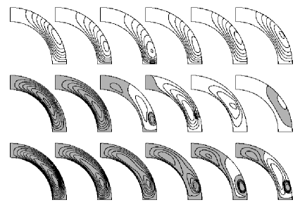
Figure 10: The structure of the $R_{B}=50$ field. The top two rows show the poloidal and toroidal fields at times 0.033, 0.067, $\ldots$, 0.2, with contour intervals of 0.025 and 0.1, respectively. The bottom row shows the toroidal field at times 0.075, 0.08, $\ldots$, 0.1, with a contour interval of 0.05, in order to see the emergence of this very intense current loop in more detail.

3.4 Initial Condition $2/3\,{\bf B}_{p1}+1/3\,{\bf B}_{p2}$

All of the solutions presented so far have belonged to one or the other of the two equatorial symmetry classes discussed in section 2.7. To get at least some idea of what might happen when these two families are allowed to interact, we (rather arbitrarily) take the initial condition $2/3\,{\bf B}_{p1}+1/3\,{\bf B}_{p2}$ (so $B_{r}(r_{o},0)=1$ is still the maximum surface field). Figures 11 and 12 show these results. A number of interesting features to note are how $b_{1}$ is still almost completely unaffected by the inclusion of Hall drift, whereas $b_{2}$ is so strongly affected that it now oscillates in sign, rather than decaying monotonically as in figure 9. The higher harmonics $b_{3}$ and $b_{4}$ are also excited, with maximum amplitude around 0.2 for both.

One could now obviously do endless more runs, for example to discover how large the initial $b_{1}$ must be to cause $b_{2}$ to oscillate, or whether a sufficiently large initial $b_{2}$ could cause $b_{1}$ to oscillate instead. However, given that there is no observational or theoretical reason to prefer any of these linear combinations over any other, that seems rather pointless. It is already evident in figure 11 that Hall drift affects mixed parity solutions in much the same way as pure parity solutions, and that is probably all we can expect to learn from these runs.

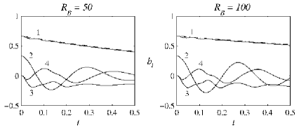
Figure 11: The harmonics $b_{1}$ through $b_{4}$ as functions of time.

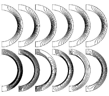
Figure 12: The structure of the $R_{B}=100$ field, at times 0.05, 0.1, $\ldots$, 0.3, with contour intervals of 0.025 and 0.05, respectively. One interesting feature to note here is how the toroidal field is dominated by the ${\bf B}_{t1}$ mode, the one that is absent in either of the pure parity families.

4 Conclusion

The results presented here suggest that Hall drift could indeed have a significant influence on the evolution of a neutron star’s magnetic field. Particularly if the internal toroidal field is as strong or stronger than the poloidal field, Hall drift can excite some of the higher harmonics to amplitudes comparable to the original mode. However, as substantial as some of these higher harmonics are, this still does not appear to be enough to cause the original mode to decay significantly faster than it otherwise would have. This conclusion must be qualified though by our inability to increase $R_{B}$ indefinitely. Indeed, the very feature that caused the code to fail beyond certain limits, namely the fact that the spectra got flatter and flatter, also indicates that this transfer of energy to the higher harmonics gets more and more efficient as $R_{B}$ is increased. It is conceivable, therefore, that the solutions for, say, $R_{B}=1000$ would show a very rapid decay of the original mode. Also, the cascade may well be very different in 3D than in 2D, just like ordinary fluid turbulence is very different. Extending our model here from 2D to 3D is possible in principle, but will obviously require considerable computational resources.

Finally, even if it should turn out that Hall drift alone, in either 2D or 3D, simply does not generate a sufficiently strong cascade at any value of $R_{B}$, the combination of Hall drift and stratification may still do so. We’ve already noted in the introduction that the electron number density $n$ in equation (2) is in fact not constant, but rather varies by several orders of magnitude over the depth of the crust. Vainshtein et al. (2000) show that if one includes this effect, one can obtain a very rapid decay of a toroidal field at least. In their highly idealized analytical model it was not possible to include poloidal fields though (we recall from section 2.4 that one can indeed consistently consider only toroidal fields). In contrast, our numerical model here already includes poloidal fields, and including radial variations in $n$ is possible too. Calculations are therefore currently under way to see if this Vainshtein et al. result applies to poloidal fields as well.

References

- [1] Bhattacharya D., 1995, JA&A, 16, 217
- [2] Bhattacharya D., Datta B., 1996, MNRAS, 282, 1059
- [3] Blondin J. M., Freese K., 1986, Nature, 323, 786
- [4] Chanmugam G., 1992, ARA&A, 30, 143
- [5] Goldreich P., Reisenegger A., 1992, ApJ, 395, 250
- [6] Hartman J. W., Bhattacharya D., Wijers R., Verbunt F., 1997, A&A, 322, 477
- [7] Hollerbach R., 2000, Int. J. Numer. Meth. Fluids, 32, 773
- [8] Jones P. B., 1988, MNRAS, 233, 875
- [9] Knobloch E., Tobias S. M., Weiss N. O., 1998, MNRAS, 297, 1123
- [10] Konenkov D. Y., Geppert U., 2001, Astron. Lett., 27, 163
- [11] Lyne A. G., 2000, Phil. Trans. R. Soc. A, 358, 831
- [12] Lyne A. G., Manchester R. N., Taylor J. H., 1985, MNRAS, 213, 613
- [13] Murakami T., 1999, Astron. Nach., 320, 257
- [14] Muslimov A. G., 1994, MNRAS, 267, 523
- [15] Muslimov A. G., Van Horn H. M., Wood M. A., 1995, ApJ, 442, 758
- [16] Naito T., Kojima Y., 1994, MNRAS, 266, 597
- [17] Narayan R., Ostriker J. P., 1990, ApJ, 352, 222
- [18] Ockendon J., Howison S., Lacey A., Movchan A., 1999, Applied Partial Differential Equations, Oxford University Press
- [19] Regimbau T., Pacheco J. A. D., 2001, A&A, 374, 182
- [20] Rheinhardt M., Geppert U., 2002, Phys. Rev. Lett., 88, 101103
- [21] Romani R. W., 1990, Nature, 347, 741
- [22] Shalybkov D. A., Urpin V. A., 1997, A&A, 321, 685
- [23] Taam R. E., van den Heuvel E. P. J., 1986, ApJ, 305, 235
- [24] Urpin V., Geppert U., 1995, MNRAS, 275, 1117
- [25] Urpin V., Shalybkov D., 1999, MNRAS, 304, 451
- [26] Vainshtein S. I., Chitre S. M., Olinto A. V., 2000, Phys. Rev. E, 61, 4422
- [27] Wijers R. A. M. J., 1997, MNRAS, 287, 607