submitted to The Astrophysical Journal
The Scattered X-Ray Halo Around Nova Cygni 1992:
Testing a Model for Interstellar Dust

Abstract

We use published ROSAT observations of the X-ray Nova V1974 Cygni 1992 to test a model for interstellar dust, consisting of a mixture of carbonaceous grains and silicate grains. The time-dependent X-ray emission from the nova is modelled as the sum of emission from a O-Ne white dwarf plus a thermal plasma, and X-ray scattering is calculated for a dust mixture with a realistic size distribution. Model results are compared with the scattered X-ray halos measured by ROSAT at 9 different epochs, including the early period of rising X-ray emission, the “plateau” phase of steady emission, and the X-ray decline at late times. We find that the observed X-ray halos appear to be consistent with the halos calculated for the size distribution of Weingartner & Draine which reproduces the Milky Way extinction with $R_{V}=3.1$, provided that the reddening to the nova is $E(B-V)\approx 0.20$, consistent with $E(B-V)\approx 0.19$ inferred from the late-time Balmer decrement. The time delay of the scattered halo relative to the direct flux from the nova is clearly detected.

Models with smoothly-distributed dust give good overall agreement with the observed scattering halo, but tend to produce somewhat more scattering than observed at 200–300″, and insufficient scattering at 50–100″. While an additional population of large grains can increase the scattered intensity at 50–100″, this could also be achieved by having $\sim$30% of the dust in a cloud at a distance from us equal to $\sim$95% of the distance to the nova. Such a model also improves agreement with the data at larger angles, and illustrates the sensitivity of X-ray scattering halos to the location of the dust. The observations therefore do not require a population of micron-sized dust grains.

Future observations by Chandra and XMM-Newton of X-ray scattering halos around extragalactic point sources can provide more stringent tests of interstellar dust models.

1 Introduction

Interstellar grains scatter X-rays through small scattering angles, and as a result distant X-ray point sources appear to be surrounded by a diffuse “halo” of scattered X-rays (Overbeck 1965; Martin 1970; Hayakawa 1973). The angular structure and absolute intensity of these scattered halos can be measured using imaging X-ray telescopes, thus providing a test for interstellar grain models (Catura 1983; Mauche & Gorenstein 1986; Mitsuda et al. 1990; Mathis & Lee 1991; Clark et al. 1994; Woo et al. 1994; Mathis et al. 1995; Predehl & Klose 1996; Smith & Dwek 1998; Witt et al. 2001; Smith et al. 2002). Given an accurate model for the dust grain size distribution and its scattering properties, observations of scattering halos can also constrain the spatial distribution of dust towards a source and the distance to a source, particularly if the emission is time variable (Trümper & Schönfelder 1973; Predehl et al. 2000).

Nova V1974 Cygni 1992, a bright X-ray nova, was observed extensively by the imaging X-ray telescope on ROSAT, resulting in the best extant data set for studies of the X-ray scattering properties of dust (Krautter et al. 1996). Mathis et al. (1995) compared model calculations to the X-ray halo observed 291 days after optical maximum, and argued that the angular structure of the observed X-ray halo favored a grain model based on highly porous grains. Smith & Dwek (1998) disagreed with this conclusion, arguing that the halo around Nova Cygni 1992 did not require porous grains, but was in fact consistent with the scattering expected from a mixture of nonporous silicate and carbon grains. More recently, Witt, Smith, & Dwek (2001) reached a different conclusion, arguing that the observed X-ray halo around Nova Cygni 1992 requires that the size distribution of interstellar dust grains extend to radii $a\geq 2.0\micron$, with $\gtrsim$40% of the dust mass in grains with radii $a>0.5\micron$.

Weingartner & Draine (2001) and Li & Draine (2001) have recently put forward a physical dust model which is in quantitative agreement with the wavelength-dependent extinction of starlight as well as the observed spectrum of infrared emission from interstellar dust. The model consists of a mixture of carbonaceous grains (including ultrasmall grains with the properties of polycyclic aromatic hydrocarbon molecules) and amorphous silicate grains. By appropriate adjustment of the size distribution, the model can reproduce the extinction in different regions of the Milky Way, and in the Large and Small Magellanic Clouds. Li & Draine (2002) show that the model is also consistent with the observed infrared emission from the Small Magellanic Cloud. Here we use the observed X-ray halo around Nova Cygni 1992 to test this dust grain model. Since the sightline toward Nova Cygni 1992 is presumably typical diffuse interstellar medium, we use the Weingartner & Draine (2001, hereafter WD01) size distribution for Milky Way dust with $R_{V}=3.1$.

In §3 we review estimates of the distance to and the gas and dust toward Nova Cygni 1992. An empirical model for the X-ray emission from the nova is described in §4, with the emission modelled as the sum of emission from a hot thermal plasma plus a white dwarf photosphere with varying temperature and radius. The methodology for calculation of X-ray scattering by dust is presented in §5, including multiple scattering, the effects of time delay, and the calculation of dust scattering cross sections.

Our results are presented in §6. We test our model using observations from 9 different epochs, at radii out to 2000″. We show that the WD01 model is in quite good agreement with the observations if the dust is assumed to follow an exponential density law and the nova is at a distance of $\sim$2.1 kpc. The time delay of the halo relative to the nova is clearly visible at late times when the nova is in decline. We discuss the uncertainties associated with possible clumping of the dust into clouds along the line-of-sight, and show that agreement with the observed halos can be improved if $\sim 30\%$ of the dust is concentrated in a cloud $\sim 100\,{\rm pc}$ from the nova. We conclude that the WD01 dust model is consistent with the observed X-ray halo toward Nova Cygni 1992, and a population of large dust grains is not required.

The distance estimate to the nova depends somewhat on the assumed density distribution of dust, and is considered in more detail in a separate paper (Draine & Tan 2003).

2 X-Ray Observations

ROSAT PSPC images of Nova Cygni 1992 for days 258, 261, 291, 434, 511, 612, 624, 635, and 650 after optical maximum were extracted from the ROSAT archive and analysed using the ESAS software package (Snowden et al. 1994). This corrects for the effects of the nonuniform detector response (particularly the shadowing by struts around 1200″) and vignetting, and excludes periods of high solar activity, allowing fairly accurate X-ray intensity profiles to be determined out to $\sim 2000-3000\arcsec$, particularly when the nova was bright. From the observation at day 650, which has the deepest exposure and the weakest nova halo, we identified the nine brightest background point sources. Excluding these sources, the azimuthally-averaged intensities and their statistical uncertainties were calculated for all annuli around the nova.

The diffuse background was estimated for each epoch by averaging over an annulus from 2800″ to 3200″, where the angular dependence of intensity was seen to be flat. Backgrounds ranged from $5.2\times 10^{-4}\>{\rm ct}\,{\rm s}^{-1}\,{\rm arcmin}^{-2}$ (day 261) to $9.9\times 10^{-4}\>{\rm ct}\,{\rm s}^{-1}\,{\rm arcmin}^{-2}$ (day 624). This scatter is most likely due to uncertainties in estimating intrumental backgrounds in the ESAS data reduction process. Background subtraction was therefore done separately for each epoch so that these systematic uncertainties would have a reduced impact on the determination of the intensity of the nova’s halo. Note, however, this method of evaluating the background forces the derived halos to artificially go to zero at 3000″. In Table 1 we list the background-subtracted count rates in selected annuli; we do not go beyond $2040\arcsec$ because uncertainties in the background correction dominate at larger angles. The error estimates in Table 1 include only statistical errors plus an estimated $\pm 10\%$ error in the background estimate for each epoch.

Table 1: X-Ray Lightcurve

epoch	$\dot{N}(<\!50\arcsec)$	$\dot{N}(50\!-\!100\arcsec)$	$\dot{N}(100\!-\!300\arcsec)$	$\dot{N}(300\!-\!960\arcsec)$	$\dot{N}(960\!-\!2040\arcsec)$
(day)	ct/s	ct/s	ct/s	ct/s	ct/s
258	$11.47\pm.04$	$0.522\pm.009$	$0.574\pm.011$	$0.93\pm.05$	$0.38\pm 0.17$
261	$15.10\pm.07$	$0.628\pm.015$	$0.619\pm.016$	$1.06\pm.04$	$0.60\pm 0.15$
291	$29.42\pm 0.11$	$1.12\pm.02$	$1.23\pm.02$	$2.14\pm.07$	$1.1\pm 0.3$
434	$68.09\pm 0.15$	$2.26\pm.03$	$2.68\pm.03$	$4.99\pm.07$	$3.0\pm 0.2$
511	$66.41\pm 0.17$	$2.45\pm.03$	$2.74\pm.04$	$5.14\pm.08$	$3.3\pm 0.2$
612	$3.68\pm.02$	$0.200\pm.005$	$0.309\pm.009$	$0.81\pm.06$	$0.8\pm 0.2$
624	$1.37\pm.02$	$.093\pm.005$	$0.168\pm.010$	$0.53\pm.07$	$0.6\pm 0.3$
635	$0.589\pm.011$	$.049\pm.003$	$.091\pm.008$	$0.31\pm.07$	$0.2_{-0.2}^{+0.3}$
650	$0.225\pm.004$	$.0251\pm.0015$	$.041\pm.006$	$0.18\pm.06$	$0.13_{-0.13}^{+0.21}$

Suppose that the point spread function (psf) has a fraction $\gamma(\theta)$ of the total counts within an angle $\theta$. At the median photon energy $E=480\,{\rm eV}$ of the detected photons, the ROSAT psf has $\gamma(50\arcsec)\approx 0.9800$ and $\gamma(100\arcsec)\approx 0.9869$ (Boese 2000). Suppose that $g(\theta)$ is the fraction of the halo photons interior to $\theta$. Then (neglecting the effect of the psf on the scattered photons) the total point source count rate is

$$\dot{N}_{\rm ps}=\frac{\dot{N}(0-50\arcsec)-\beta\dot{N}(50\arcsec-100\arcsec)}{\gamma(50\arcsec)-\left[\gamma(100\arcsec)-\gamma(50\arcsec)\right]\beta}~{}~{}~{},$$ (1)

$$\beta=\frac{g(50\arcsec)}{g(100\arcsec)-g(50\arcsec)}~{}~{}~{}.$$ (2)

A uniform surface-brightness halo would have $\beta=1/3$, but halos for continuously-distributed dust have $g(\theta)\propto\theta$ for $\theta\rightarrow 0$ (Draine 2003b), corresponding to $\beta=1$ if this behavior applied out to $100\arcsec$. We take $\beta\approx 0.9$ as providing a good approximation to the actual models.

Table 2 presents our derived point source count rate $\dot{N}_{\rm ps}$, the estimated halo count rate $\dot{N}_{\rm halo}$ (including only halo angles $\theta<2040\arcsec$), and the ratio $\dot{N}_{\rm halo}/\dot{N}_{\rm ps}$ of halo counts to point source counts. Note that $\dot{N}_{\rm halo}/\dot{N}_{\rm ps}$ becomes quite large at late times – this is because the point source count rate is declining rapidly, but the longer light travel time means that the halo photons were emitted from the nova at an earlier (more luminous) time than the unscattered photons.

Table 2: Point Source and Halo Components

epoch	$\dot{N}_{ps}$	$\dot{N}_{halo}$	$\dot{N}_{halo}/\dot{N}_{ps}$
(days)	ct/s	ct/s
258	$11.30\pm.05$	$2.6\pm 0.2$	$0.23\pm.02$
261	$14.93\pm.08$	$3.1\pm 0.2$	$0.206\pm.013$
291	$29.18\pm 0.12$	$5.8\pm 0.3$	$0.200\pm.011$
434	$67.84\pm 0.16$	$13.2\pm 0.3$	$0.195\pm.005$
511	$65.93\pm 0.18$	$14.1\pm 0.3$	$0.213\pm.005$
612	$3.59\pm.02$	$2.2\pm 0.3$	$0.62\pm.08$
624	$1.32\pm.02$	$1.4\pm 0.4$	$1.1\pm 0.3$
635	$0.560\pm.012$	$0.7\pm 0.3$	$1.2\pm 0.6$
650	$0.208\pm.004$	$0.40\pm 0.28$	$1.9\pm 1.3$

At times $t\leq 511$, the ratio of halo to point source is approximately constant. Because day 511 appears to have been preceded by $\sim$100 days of nearly constant X-ray luminosity, the observed halo at day 511 can be interpreted as due to steady illumination, and we can estimate the dust scattering optical depth to be

$$\tau_{\rm sca}(\theta<2040\arcsec)\approx\ln\left[1+\left(\dot{N}_{\rm halo}/\dot{N}_{\rm ps}\right)_{511}\right]\approx 0.193\pm 0.004$$ (3)

at a characteristic energy $E\approx 480\,{\rm eV}$. Based on the modelling discussed below, we estimate that $\sim$91.6$\pm 2\%$ of the halo is at $\theta<2040\arcsec$; the total X-ray scattering optical depth toward nova Cygni 1992 is therefore $\tau_{\rm sca}\approx 0.211\pm.006$

3 Distance and Gas Distribution

Nova Cygni 1992 ($\alpha_{2000}=20^{h}30^{m}31.^{s}76$, $\delta_{2000}=+52^{o}37^{\prime}52.^{\prime\prime}9$; Austin et al. 1996) has Galactic coordinates $l=89.1^{\circ}$, $b=7.82^{\circ}$ and is located at a height $Z_{\star}=D\sin b=272(D/2\,{\rm kpc})\,{\rm pc}$ above the Galactic plane. The distance $D$ has been controversial, with recent estimates $3.2\pm 0.5\,{\rm kpc}$ (Paresce et al. 1994), $D=2.1\pm 0.7\,{\rm kpc}$ (Austin et al. 1996), $1.8\pm 0.1\,{\rm kpc}$ (Chochol et al. 1997), and $D=2.6\pm 0.25\,{\rm kpc}$ (Balman et al. 1998).

To calculate X-ray scattering by dust, we require a model for the spatial distribution of dust between us and the nova. We take the Sun to be located at the Galactic midplane, $z=0$. We model the distribution of interstellar gas by an exponential distribution:

$$n_{\rm H}(z)=\frac{N_{\rm H}^{\rm ISM}(\infty)\sin b}{h_{e}}\exp(-z/h_{e}),~{}~{}~{}h_{e}=\frac{z_{1/2}}{\ln 2}~{}~{}~{},$$ (4)

$$N_{\rm H}^{\rm ISM}(D)=N_{\rm H}^{\rm ISM}(\infty)\left[1-\exp(-D\sin b/h_{e})\right]~{}~{}~{},$$ (5)

where $z$ is the height above the Galactic plane, and $z_{1/2}$ is the height where the density is 50% of the maximum value.

H I 21 cm emission maps of this region (Hartmann & Burton 1997) indicate a total atomic H column density $N({\rm H~{}I})=2.2\times 10^{21}\,{\rm cm}^{-2}$ within $\sim$5 kpc (integration performed from $-50\,{\rm km~{}s}^{-1}<v_{\rm lsr}<+50\,{\rm km~{}s}^{-1}$; a weak component at $-150\,{\rm km~{}s}^{-1}<v_{\rm lsr}<-50\,{\rm km~{}s}^{-1}$ is excluded), if the emission is optically thin. From the COBE and DIRBE far-infrared maps, Schlegel et al. (1998) estimate a total dust column with $E(B-V)=0.412$ mag; with the local ratio $N_{\rm H}/E(B-V)=5.8\times 10^{21}\,{\rm cm}^{-2}$ (Bohlin, Savage, & Drake 1978) this corresponds to $N_{\rm H}^{\rm ISM}(\infty)=2.39\times 10^{21}\,{\rm cm}^{-2}$, which we adopt as our best estimate in the direction of the nova.

Based on studies of the vertical distribution of the gas (see Binney & Merrifield 1998, Fig. 9.25) we adopt a half-density height $z_{1/2}=300$ pc for the gas at Galactocentric radius $R_{0}<R<1.03R_{0}$. This gives a midplane density $n_{\rm H}(0)=N_{\rm H}^{\rm ISM}(\infty)\sin b/h_{e}=0.24\,{\rm cm}^{-3}$. We will also consider $z_{1/2}=250\,{\rm pc}$ and $350\,{\rm pc}$ for comparison.

Given an adopted density law, we treat the distance $D$ to the nova as an adjustable parameter which determines the column of dust and gas between us and the nova, which in turn determines the strength of the scattering halo relative to the X-ray point source. By comparing models with different $D$, we will determine what column density $N_{\rm H}^{\rm ISM}(D)$ best reproduces the observed strength of the scattering halo.

3.1 Attenuation by Gas and Dust

Radiation from the nova is attenuated by gas and dust along the line of sight. From the ROSAT data, Balman et al. (1998) find that the observed flux from the nova is consistent with emission from hot plasma plus a white dwarf photosphere, attenuated by absorption by interstellar gas with column density $N_{\rm H}\approx 2.1\times 10^{21}\,{\rm cm}^{-2}$ at late times ($t\gtrsim 255\,{\rm d}$), but with additional absorption at earlier times.

Our objective is simply to find an empirical description which reproduces the observed count rate and energy spectrum of unscattered photons arriving at the Earth. To this end we adopt the parameters estimated by Balman et al. The results of Balman et al. appear to be consistent with time-dependent absorption by

$$N_{\rm H}^{\rm abs}(t) = 2.1\times 10^{21}\left(\frac{255\,{\rm d}}{t}\right)^{2}\,{\rm cm}^{-2}~{}~{}~{}{\rm for}~{}t<255\,{\rm d}$$ (6)

$$= 2.1\times 10^{21}\,{\rm cm}^{-2}~{}~{}~{}{\rm for}~{}t>255\,{\rm d}~{}~{}.$$ (7)

The decline of $N_{\rm H}^{\rm abs}$ with time is presumed to be due to the combined effects of expansion and ionization of gas associated with the nova. We will assume that the absorption is due to the interstellar contribution $N_{\rm H}^{\rm ISM}$ [eq. (5)] plus a time-variable

$$\Delta N_{\rm H}(t)=N_{\rm H}^{\rm abs}(t)-N_{\rm H}^{\rm ISM}$$ (8)

contributed by gas associated with the nova.

We will see below that the observed X-ray halo appears to be consistent with models with $N_{\rm H}^{\rm ISM}\approx 1.0\times 10^{21}\,{\rm cm}^{-2}$ between us and the nova. The absorption optical depth of the interstellar gas is shown in Fig. 1 as a function of energy, for $N_{\rm H}^{\rm ISM}=1.0\times 10^{21}\,{\rm cm}^{-2}$. Photoelectric absorption due to H, He, C, N, O, Ne, Mg, Si, S, and Fe is included, with cross sections calculated following Verner and Yakovlev (1995) and Verner et al. (1996), using subroutine phfit2.f written by D.A. Verner (1996).

In the interstellar gas, abundances relative to H are taken to be 100% of solar for He I, N I, Ne I, and S II, 30% of solar for C II, 80% of solar for O I, and 10% of solar for Mg II, Si II, and Fe II due to depletion into dust grains. Nova Cygni 1992 did not form dust in the ejecta (Woodward et al. 1997). In the circumstellar material we assume no dust grains, and solar abundances for He I, C II, N I, O I, Ne I, Mg II, Si II, S II, and Fe II. Solar abundances for He, N, Ne, S are from Grevesse & Sauval (1998); for Si and Fe from Asplund (2000); for C from Allende Prieto et al. (2002a); for O from Allende Prieto et al. (2002b).

In addition to gas phase absorption, there is absorption and scattering by interstellar dust grains. This is calculated assuming a mixture of carbonaceous grains and silicate grains, with the “case A” size distribution found by WD01 for Milky Way dust with $R_{V}\equiv A_{V}/E(B-V)=3.1$, but with grain abundance per H nucleon reduced by a factor 0.93, as recommended by Draine (2003a). Absorption and scattering cross sections were calculated using dielectric functions which include structure near the X-ray absorption edges (Draine 2003b), as described in §5.

Extinction and scattering optical depths for this dust are shown in Fig. 1 as functions of photon energy, for a sightline with $N_{\rm H}^{\rm ISM}=1.0\times 10^{21}\,{\rm cm}^{-2}$. Below $\sim 0.5\,{\rm keV}$ absorption by the gas dominates, since H and He are both assumed to be neutral. At $\sim 0.8\,{\rm keV}$ the dust grains provide $\sim$50% of the extinction, and at energies above $1\,{\rm keV}$ the dust grains dominate the extinction.

The interstellar matter ($N_{\rm H}^{\rm ISM}$) and the circumstellar gas ($\Delta N_{\rm H}$) are taken to have differing attenuation properties, since some of the interstellar matter (but none of the circumstellar material) is in the form of dust grains. Our estimate for the total attenuation therefore depends on the fraction of the total column contributed by the interstellar medium, and this in turn depends on the assumed distance $D$.

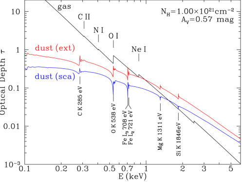
Figure 1: Optical depths due to photoelectric absorption by interstellar gas and extinction by dust, for a sightline with $N_{\rm H}^{\rm ISM}=1.0\times 10^{21}\,{\rm cm}^{-2}$. Also shown is the contribution to dust extinction due to scattering. Photoelectric absorption edges are indicated for C II, N I, O I, and Ne I.

4 X-Ray Spectrum of Nova V1974 Cygni 1992

Scattering of X-rays by dust grains is a function of the X-ray energy, so it is important to use a realistic source spectrum when modelling this phenomenon. Mathis et al. (1995) approximated the emission as a blackbody with $kT=22\,{\rm eV}$, attenuated by foreground gas with $N_{\rm H}=4.25\times 10^{21}\,{\rm cm}^{-2}$ and solar abundances, while Witt et al. (2001) approximated the spectrum by a delta function with $E=400\,{\rm eV}$.

Balman, Krautter & Ögelman (1998) have recently examined the lightcurve and spectrum of Nova Cygni 1992, and find that it appears to be the sum of two separate components: thermal emission from the photosphere of the white dwarf, with effective temperature $T_{\rm wd}$ and radius $R_{\rm wd}$ both varying in time, plus emission from a cooling and expanding thermal plasma. We adopt this two-component model for the point-source flux $F_{\nu}$:

$$F_{\nu}(t)=\left[F_{\nu}^{\rm pl}(t)+F_{\nu}^{\rm wd}(t)\right]\exp\left[-\tau_{\rm abs,gas}(\nu)-\tau_{\rm abs,dust}(\nu)-\tau_{\rm sca}(\nu)\right]~{}~{}~{}.$$ (9)

4.1 Thermal Plasma

The flux $F_{\nu}^{\rm pl}$ from the emitting plasma is

$$F_{\nu}^{\rm pl}=\frac{1}{4\pi D^{2}}\int n_{e}n_{\rm H}dV\frac{\Lambda_{\nu}(T_{\rm pl})}{n_{e}n_{\rm H}}$$ (10)

where $\Lambda_{\nu}(T_{\rm pl})$, the power radiated per unit volume and unit frequency by an optically-thin thermal plasma with kinetic temperature $T_{\rm pl}$, is calculated using the Raymond & Smith (1977) code for a solar abundance plasma in collisional ionization equilibrium.

We take the plasma properties to be given by

$$T_{\rm pl}=\left\{\begin{array}[]{ll}10^{8}\,{\rm K}&t<63\,{\rm d}\\ 10^{8}\,{\rm K}\left[1-0.9(t-63\,{\rm d})/42\,{\rm d}\right]&63\,{\rm d}<t<105\,{\rm d}\\ 10^{7}\,{\rm K}&t>105\,{\rm d}\end{array}\right.$$ (11)

$$\frac{1}{4\pi D^{2}}\int n_{e}n_{\rm H}dV=1.44\times 10^{12}A_{\rm pl}\,{\rm cm}^{-5}\left\{\begin{array}[]{ll}(t/94\,{\rm d})^{2}&t\leq 94\,{\rm d}\\ (t/94\,{\rm d})^{-2}&t>94\,{\rm d}\end{array}\right.$$ (12)

with a correction factor

$$A_{\rm pl}=\exp\left[0.0925\left(\frac{N_{\rm H}^{\rm ISM}}{10^{21}\,{\rm cm}^{-2}}-1.0\right)\right]$$ (13)

depending on the assumed value of $N_{\rm H}^{\rm ISM}$. The adopted plasma temperature (eq. 11) is consistent with the temperature of this component inferred by Balman et al., and eq. (12) reproduces the PSPC count rates at times $t\leq 147\,{\rm d}$

4.2 Nova Photosphere

Balman et al. found that the emission from the nova photosphere was consistent with the spectrum calculated by MacDonald & Vennes (1991) for O-Ne enhanced white dwarf model atmospheres. Following Balman et al., we approximate the emission from the nova photosphere using the O-Ne enhanced white dwarf model atmosphere spectra of MacDonald & Vennes (1991). We will assume that the light curve consists of three phases: (1) at times $t<t_{p1}$, the atmosphere is contracting at constant luminosity, with the temperature rising; (2) at times $t_{p1}<t<t_{p2}$, the atmospheric radius remains constant, with the temperature nearly constant (the “plateau” phase); (3) at $t>t_{p2}$ the nova has exhausted its fuel, and the photosphere begins to cool rapidly at constant radius.

The beginning and end of the plateau phase are not well determined by the ROSAT observations. We will assume that the plateau phase began at $t_{p1}=335\,{\rm d}$, and ended at $t_{p2}=565\,{\rm d}$. The highest observed count rate was at $t=434\,{\rm d}$, at which time we assume an effective temperature $kT_{\rm wd}=50\,{\rm eV}$; the ROSAT point source count rate (see §4.3) on day 434 can be reproduced if

$$\pi\left(\frac{R_{\rm wd}}{D}\right)^{2}=2.61\times 10^{-25}A_{\rm wd}\,{\rm sr}~{}~{}~{}{\rm for}~{}t>t_{p1}$$ (14)

with a correction factor

$$A_{\rm wd}=\exp\left[0.198\left(\frac{N_{\rm H}^{\rm ISM}}{10^{21}\,{\rm cm}^{-2}}-1.0\right)\right]$$ (15)

which depends weakly on the adopted value of $N_{\rm H}^{\rm ISM}$. With the assumption of $R_{\rm wd}=$ constant for $t\geq t_{p1}$, we determine the effective temperature $kT_{\rm wd}=49.84\,{\rm eV}$ on day 511. We assume $dT_{\rm wd}/dt$ to be constant throughout the plateau phase, giving $kT_{p1}=50.16\,{\rm eV}$, and $kT_{p2}=49.72\,{\rm eV}$. The peak luminosity is reached at $t_{p1}$:

$$L_{\rm wd}=2.57\times 10^{38}A_{\rm wd}\left(\frac{D}{2.0\,{\rm kpc}}\right)^{2}\,{\rm ergs}\,{\rm s}^{-1}~{}~{}~{}.$$ (16)

At times $t<t_{p1}$ the nova radius is obtained by assuming constant luminosity:

$$\pi\left(\frac{R_{\rm wd}}{D}\right)^{2}=2.61\times 10^{-25}\left(\frac{kT_{p1}}{kT_{\rm wd}}\right)^{4}~{}~{}~{}{\rm for}~{}t<t_{p1}~{}~{}~{}.$$ (17)

For $t=258$, 261, 612, 624, 635, and 650 days we determine $T_{\rm wd}$ by requiring that we reproduce the observed $\dot{N}_{ps}$, for constant luminosity at $t<t_{p1}$, and constant radius for $t>t_{p1}$. For $t\leq 258\,{\rm d}$, we assume $T\propto t$.

Tabulated model atmosphere spectra have been obtained from MacDonald (2002) for temperatures $T_{\rm wd}=1,2,3,3.5,4,5,6\times 10^{5}\,{\rm K}$; we estimate the spectrum at intermediate temperatures by interpolation.

4.3 Model Count Rate

Our aim is to reproduce the ROSAT counts as a function of halo angle. We must first ensure that our nova model reproduces the observed count rates for the point-source component. For the nova model and interstellar medium parameters described above, we calculate the rate of 0.1 – 2.4 keV photon detections by the ROSAT PSPC. We use the ROSAT effective area vs. energy from Snowden et al. (1994).

In Figure 2 we show the ROSAT point-source count rate calculated for our model for the nova and intervening extinction, together with measured count rates.

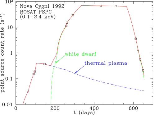
Figure 2: Light curve for point source component of Nova Cygni 1992. Solid line: count rate for two component model, including attenuation by gas and dust. Broken curves: contributions from thermal plasma and white dwarf photosphere. Squares: measured count rates from Krautter et al. (1996) for $t\leq 147\,{\rm d}$, and from Table 1 for $t\geq 258\,{\rm d}$.

In Figure 3 we show the calculated energy spectrum of detected photons at 4 different times. We note that the energy spectrum varies considerably over the evolution of the nova. At $t=91\,{\rm d}$ the spectrum is quite hard, being dominated by the thermal emission from hot plasma with $kT_{\rm pl}\approx 3.4\,{\rm keV}$. At this time the white dwarf photosphere is relatively cool, and the radiation from it is absorbed by intervening H and He. As the white dwarf photosphere contracts and becomes hotter, its 0.2–0.7 keV emission comes to dominate the count rate (see, e.g., the spectra for $t=258$, 434, and $635\,{\rm d}$ in Figure 3).

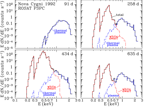
Figure 3: ROSAT PSPC count rates as function of photon energy for two-component model for Nova Cygni 1992, including extinction by gas and dust, for $N_{\rm H}^{\rm ISM}=1.15\times 10^{21}\,{\rm cm}^{-2}$.

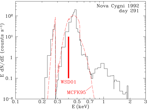
Figure 4: ROSAT PSPC count rate spectrum as function of photon energy for day 291. Present model (solid histogram) is compared with count rate spectrum adopted by Mathis et al. (1995) (MCFK95) and the representative photon energy used by Witt et al. (2001) (WSD01). The drop in count rate at 284 eV is due to absorption by C in the ROSAT window.

In Fig. 4 we display the energy spectrum of detected photons at $t=291\,{\rm d}$ after optical maximum, together with the spectra used by Mathis et al. (1995) and Witt et al. (2001).

5 X-Ray Scattering

The theoretical framework for calculation of scattered halos around X-ray sources has been discussed by Mauche & Gorenstein (1986), Mitsuda et al. (1990), Mathis & Lee (1991), and Predehl & Klose (1996). The treatment which we present here is fully general, subject to only the following approximations:

1. Polarization is neglected. This is an excellent approximation for X-rays since scattering is only appreciable for small scattering angles ($\lesssim 1^{\circ}$) for which polarization effects are negligible.

2. Dust grains are assumed to be randomly-oriented. If dust grains are nonspherical and preferentially aligned, the dust scattering halo would not be azimuthally symmetric. While it may be possible to detect this effect in future observational studies, we neglect it in the present treatment. Generalization to include this effect would be straightforward but cumbersome, and not merited at this time.

3. We assume that the extinction (scattering by dust plus absorption by gas and dust) along each path contributing to the scattered intensity is the same as the extinction along the direct line from observer to source. Since the scattering halos are small ($\sim$90% of the scattered photons within $\sim 0.5^{\circ}$) this is quite a good approximation. Towards Nova Cygni 1992 there are variations in $N_{\rm H}^{\rm ISM}(\infty)$ of $\sim 20\%$ on $0.5^{\circ}$ scales, particularly in a direction perpendicular to the Galactic plane (Hartmann & Burton 1997). In the optically-thin limit (i.e. for $h\nu\gtrsim 1\,{\rm keV}$, see Fig. 1), such a density gradient has no effect on the azimuthally-averaged halo intensity, relative to uniform extinction with a column equal to the average over the halo scale in the inhomogeneous case. When the optical depth is $\sim 1$ (i.e. for $h\nu\sim 500\,{\rm eV}$), the differential absorption makes a small ($\sim 1\%$) effect on the azimuthally-averaged profiles compared to the uniform case.

4. It is assumed that photons scattered by more than $90^{\circ}$ may be neglected: we only consider scattered photons travelling away from the source (the “outward-only approximation”).

5. The dust is assumed to be distributed spherically-symmetrically around the source. For example, there could be a spherical cavity surrounding the source. Outside of this cavity, when we use a prescription (e.g., exponential density law) for the dust density, we take this to be the density along the sightline to the nova; the assumed spherical symmetry provides densities away from the sightline. Within the small halo angles $\lesssim 1^{\circ}$ of interest, the resulting densities are close to what would have been obtained for the plane-parallel density structure which is the basis for our original density estimate. The assumed spherical symmetry implies azimuthal symmetry around the sightline to the source. Predehl & Schmitt (1995) found that X-ray halos in ROSAT observations did not show any detectable azimuthal asymmetries.

Our formulae are presented without the small-angle approximations which are frequently found in discussions of X-ray scattering by dust.

Consider a point source of specific luminosity $L_{\nu}$ at a distance $D$ from the observer, and let $r$ be the distance along the line from the observer to the source. We assume the the dust size distribution and composition are the same everywhere, but the dust spatial density $\rho$ may vary along the line of sight.

Let $\tau_{\rm abs}$ and $\tau_{\rm sca}$ be the total optical depths for scattering and extinction from source to observer. At a distance $r=xD$ along the line from observer to the point source, and at “retarded” time $t$ (time measured relative to the arrival of a fiducial pulse emitted by the source), the intensity of $n-$times scattered photons arriving from an angle $\theta$ is given by

$$I_{n,\nu}(r,t,\theta)=\frac{L_{\nu}(t)}{4\pi D^{2}}~{}e^{-\tau_{\rm abs}}\frac{e^{-\tau_{\rm sca}}~{}\tau_{\rm sca}^{n}}{n!}~{}\tilde{I}_{n}(x=r/D,t,\theta)~{}~{}~{}.$$ (18)

Eq. (18) serves to define $\tilde{I}_{n}(x,t,\theta)$, which depends on the dust distribution along the line-of-sight, but not on the quantity of dust present. The normalization is such that in the approximation of small scattering angles, for a steady source one has $\int\tilde{I}_{n}(0,t,\theta)2\pi\sin\theta d\theta=1$.

Figure 5: Geometry [upper panel] for calculation of normalized single scattering intensity $I_{1}(x,\theta)$ and [lower panel] for calculation of multiple scattering intensity $I_{n}(x,\theta)$ given $I_{n-1}(y,\alpha)$ for $y>x$. The observer is at $x=0$.

5.1 Single Scattering

For single-scattering (see Fig. 5) the dimensionless intensity function $\tilde{I}_{1}$ is given by

$$\tilde{I}_{1}(x,t,\theta)=\frac{1}{\cos\theta}\int_{x}^{1}dy\frac{\tilde{\rho}(y^{\prime})\tilde{\sigma}({\Theta_{s}})}{(1-y)^{2}+(y-x)^{2}\tan^{2}\theta}\frac{L_{\nu}(t-\delta t_{1}(x,y,\theta))}{L_{\nu}(t)}$$ (19)

where

$$y^{\prime}\equiv 1-\sqrt{(1-y)^{2}+y^{2}\tan^{2}\theta}$$ (20)

and the dimensionless density is

$$\tilde{\rho}(x)\equiv\frac{\rho(r=xD)}{D^{-1}\int_{0}^{D}\rho(r)dr}~{}~{}~{}.$$ (21)

The dimensionless differential scattering cross section is

$$\tilde{\sigma}({\Theta_{s}})\equiv\frac{1}{\sigma_{sca}}\frac{d\sigma}{d\Omega}~{}~{}~{},$$ (22)

where $d\sigma/d\Omega$ is the differential scattering cross section for scattering angle

$${\Theta_{s}}(x,y,\theta)=\psi_{0}(x,y,\theta)$$ (23)

where

$$\psi_{0}(x,y,\theta)\equiv\theta+\arctan\left[\frac{(y-x)\tan\theta}{1-y}\right],$$ (24)

and the time delay

$$\delta t_{1}(x,y,\theta) = \frac{D}{c}\left\{\frac{y-x}{\cos\theta}+(1-y)\left[1+\left(\frac{y-x}{1-y}\right)^{2}\tan^{2}\theta\right]^{1/2}-(1-x)\right\}$$ (25)

$$\approx \frac{D}{c}\frac{(1-x)(y-x)}{(1-y)}\frac{\theta^{2}}{2}=28.0\,{\rm d}\left(\frac{D}{2.0\,{\rm kpc}}\right)\frac{(1-x)(y-x)}{(1-y)}\left(\frac{\theta}{1000\arcsec}\right)^{2}.$$ (26)

For a steady source,

$$\tilde{I}_{1}\rightarrow\tilde{I}_{1}^{\rm s}(x,\theta)\equiv\frac{1}{\cos\theta}\int_{x}^{1}dy\frac{\tilde{\rho}(y^{\prime})\tilde{\sigma}({\Theta_{s}})}{(1-y)^{2}+(y-x)^{2}\tan^{2}\theta}~{}~{}~{}.$$ (27)

5.2 Multiple Scattering

For a steady source, the intensity of multiply-scattered photons is obtained from the recursion formula (Mathis & Lee 1991; Predehl & Klose 1996)

$$\tilde{I}_{n}^{\rm s}(x,\theta)=\frac{n}{\cos\theta}\int_{x}^{1}dy~{}\tilde{\rho}(y^{\prime})\int_{0}^{{\pi/2}}d\alpha\sin\alpha~{}\tilde{I}_{n-1}^{\rm s}(y,\alpha)\int_{0}^{2\pi}d\beta~{}\tilde{\sigma}({\Theta_{s}})~{}~{}~{}(n\geq 2),$$ (28)

where the scattering angle

$${\Theta_{s}}(x,y,\theta,\alpha,\beta)=\arccos\left(\cos\alpha\cos\psi_{0}+\sin\alpha\cos\beta\sin\psi_{0}\right)~{}~{}~{}.$$ (29)

The upper limit $\pi/2$ on the integral over $\alpha$ corresponds to the “outward-only” approximation mentioned above. For a nonsteady source, it is possible to allow exactly for the time delays on different light paths, but the formalism becomes cumbersome and the computations burdensome. In the present application multiple scattering is a relatively minor effect, and time delay is a relatively minor correction, so for $n\geq 2$ we make only an approximate correction for time delay by assuming that the first $n-1$ scatterings occur exactly midway between the source and the last scattering:

$$\tilde{I}_{n}(x,t,\theta)\approx\frac{n}{\cos\theta}\int_{x}^{1}dy~{}\tilde{\rho}(y^{\prime})\int_{0}^{{\pi/2}}d\alpha\sin\alpha~{}\tilde{I}_{n-1}^{\rm s}(y,\alpha)\left[\frac{L_{\nu}(t-\delta t_{2})}{L_{\nu}(t)}\right]\int_{0}^{2\pi}d\beta~{}\tilde{\sigma}({\Theta_{s}})~{}~{}~{},$$ (30)

$$\delta t_{2}(x,\theta,\alpha) = \frac{D}{c}\left\{\frac{x}{\cos\theta}+\frac{\left[(1-x)^{2}+x^{2}\tan^{2}\theta\right]^{1/2}}{\cos\alpha}-1\right\}$$ (31)

$$\approx \frac{D}{2c}\left[\frac{x}{(1-x)}\theta^{2}+(1-x)\alpha^{2}\right]~{}~{}~{}.$$ (32)

To calculate the intensity $I_{n}(0,t,\theta)$ of $n$-times scattered photons at $x=0$, we precalculate and tabulate $\tilde{I}_{n-1}^{s}(y,\theta)$ at selected values of $y$ and $\theta$, and then obtain $\tilde{I}_{n-1}^{s}$ by interpolation when evaluating eq. (30) for $\tilde{I}_{n}(0,x,t)$.

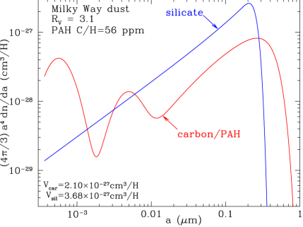
Figure 6: WD01 size distributions for carbonaceous grains (including PAHs) and amorphous silicate grains for Milky Way dust with $R_{V}=3.1$ and C/H=60ppm in PAHs. Total volume of carbonaceous grains and silicate grains per H is $2.26\times 10^{-27}$ and $3.96\times 10^{-27}\,{\rm cm}^{3}$, respectively.

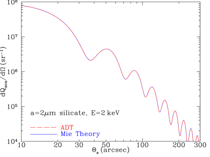
Figure 7: Differential scattering cross section calculated using Mie theory and anomalous diffraction theory for $a=2\micron$ silicate grain at 2 keV, for which $x=2.03\times 10^{4}$. The two curves are indistinguishable.

5.3 Dust Model and Scattering Cross Sections

For the line of sight to Nova Cygni 1992, we assume that the dust is “average” diffuse cloud dust, and we adopt the dust model developed by WD01 for $R_{V}\equiv A_{V}/E(B-V)\approx 3.1$ and C/H = 60 ppm in polycyclic aromatic hydrocarbons (PAHs), except that, following Draine (2003a), the abundances of all grain components (relative to H) are reduced, by a factor 0.93; with this adjustment, the grain model reproduces the estimated extinction per H nucleon. The model consists of a mixture of carbonaceous grains and amorphous silicate grains. As discussed by Li & Draine (2001), the carbonaceous grains have the properties of PAH molecules when they contain $\lesssim 10^{4}$ C atoms, and the properties of graphite particles when they contain $\gtrsim 10^{5}$ C atoms. By altering the size distributions of the carbonaceous and silicate particles, the dust model appears to be able to reproduce observed extinction curves in various Galactic regions, and in the Large and Small Magellanic Clouds. This dust model, when illuminated by starlight, produces infrared emission consistent with the observed emission spectrum of the interstellar medium (Li & Draine 2001, 2002). The size distribution for this dust model is shown in Fig. 6. For assumed densities of $2.2\,{\rm g}\,{\rm cm}^{-3}$ for the carbonaceous grains and $3.8\,{\rm g}\,{\rm cm}^{-3}$ for the MgFeSiO₄ silicate grains, this corresponds to a dust-to-gas mass ratio of 0.008

The scattering properties of a spherical target of radius $a$ are determined by the complex refractive index $m(\lambda)$ and the dimensionless size parameter $x\equiv 2\pi a/\lambda$. Many early papers on X-ray scattering by dust employed the “Rayleigh-Gans” approximation to calculate the differential scattering cross sections. Smith & Dwek (1998) showed, however, that the Rayleigh-Gans validity criterion $|m-1|x\ll 1$ is not satisfied for interstellar grains at energies $\lesssim$1 keV. In the present work we assume spherical, homogeneous grains and use exact Mie scattering theory (see, e.g. Bohren & Huffman 1984) to calculate differential scattering cross sections $d\sigma/d\Omega$, employing a computer code based upon the subroutine MIEV0 written by Wiscombe (1980, 1996), modified to use IEEE 64 bit arithmetic. Wiscombe’s code is accurate for “size parameters” $x=7800(a/\micron)(\,{\rm keV}/h\nu)<2\times 10^{4}$. For $x>2\times 10^{4}$ we calculate $d\sigma/d\Omega$ using “anomalous diffraction theory” (van de Hulst 1957), since the validity criteria $x\gg 1$ and $|m-1|\ll 1$ are satisfied. The accuracy of the scattering calculations is illustrated in Fig. 7, where we show the differential scattering cross section calculated for a case with $x=2\times 10^{4}$ – the Mie theory calculation and the anomalous diffraction theory calculation are indistinguishable. Since the two calculations are entirely different in approach, the agreement confirms that both are accurate.

For the amorphous silicate grains and the carbonaceous grains we employed the dielectric functions estimated by Draine (2003b) for olivine MgFeSiO₄ and graphite, respectively. Figure 8 shows the differential scattering cross section per H nucleon for the dust mixture of WD01 for Milky Way dust with $R_{V}=3.1$ (with grain abundances reduced by a factor 0.93). For this mixture we see that the scattering for scattering angles $\Theta_{s}<1000$″ is dominated by grains with radii in the $0.1-0.4\micron$ range – larger grains contribute only $\sim$20% of the total scattering cross section for $\Theta_{s}\lesssim 200$″, and $\lesssim 1$% for $\Theta_{s}\gtrsim 500$″. We also see that silicate grains provide $\sim$60% of the scattering for $\Theta_{s}\lesssim 300$″, increasing to $\sim$80% at $\Theta_{s}\gtrsim 1000$″.

It is well-known that the extinction curve varies from one region to another, which is presumed to be due to changes in the size distribution of the dust. In addition to the size distribution which reproduces the standard Milky Way diffuse cloud extinction curve with $R_{V}=3.1$, WD01 have constructed a size distribution consistent with an extinction curve with $R_{V}=5.5$. Such flat extinction curves are found in dense regions, and require a shift of the dust size distribution toward larger sizes. The X-ray scattering properties for dust with $R_{V}=3.1$ and 5.5 are compared in Fig. 9 – we see that $R_{V}=5.5$ dust is slightly more forward-scattering than $R_{V}=3.1$ dust. The cross section for a scattering angle of $\lesssim 300\arcsec$ is larger by about a factor 1.4.

The scattering also depends on the X-ray energy. In Fig. 9 we show the differential scattering properties of $R_{V}=3.1$ dust at energies ranging from 0.1 to 1 keV. As the energy increases, the dust becomes more forward-scattering.

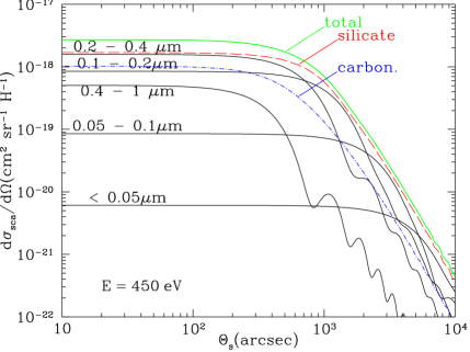
Figure 8: Heavy solid curve: differential scattering cross section per H at $h\nu=450\,{\rm eV}$ for the WD01 model for Milky Way dust with $R_{V}=3.1$ and C/H=60 ppm in PAHs. Also shown are separate contributions of silicate and carbonaceous grains, and contributions from different size ranges.

Figure 9: Upper panel: differential scattering cross section at $E=450\,{\rm eV}$ for WD01 model for Milky Way dust with $R_{V}=3.1$ (diffuse cloud average) and $R_{V}=5.5$ (dense cloud). Lower panel: differential scattering cross sections at 8 energies for WD01 model for Milky Way dust with $R_{V}=3.1$.

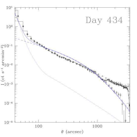
Figure 10: X-ray intensity profile from Nova Cygni 1992, 434 days after optical maximum. Solid histogram: raw ROSAT PSPC data in 10″bins. Triangles: intensities after processing by ESAS software (see text). The background is determined by averaging the intensity in the annulus from 2800-3200″. Squares: nova intensity after background subtraction. The error bar around each point shows the $3-\sigma$ statistical error but does not include any uncertainty due to background subtraction. Solid curve: model intensity profile [psf (dotted line) plus dust-scattered halo (dashed line)] for nova at $D=2.1\,{\rm kpc}$. The model is in generally good agreement over the full 40–3000″range where the scattered halo can be measured, but overpredicts the scattered intensity by $\sim$40% at $\theta\approx 250$″, and underpredicts the observed intensity at $\theta<100\arcsec$.

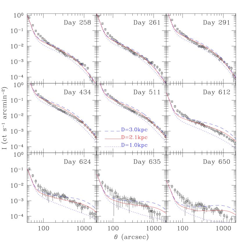
Figure 11: Multi-epoch X-ray intensity profiles from Nova Cygni 1992. Squares: observed intensity profile; the error bar shows the $3-\sigma$ statistical uncertainty. Solid lines: models consisting of psf plus dust-scattered halo for exponential density law with $z_{1/2}=300\,{\rm pc}$ and nova at an assumed distance of $D=2.1\,{\rm kpc}$. This distance, corresponding to $N_{\rm H}^{\rm ISM}=1.15\times 10^{21}\,{\rm cm}^{-2}$, or $E(B-V)=0.20$ mag, gives the best overall match to the data. Dotted lines: the same models but for $D=1.0$ (lower line) and $3.0\,{\rm kpc}$ (upper line) (corresponding to $N_{\rm H}^{\rm ISM}=0.64$ and $1.46\times 10^{21}\,{\rm cm}^{-2}$, or $E(B-V)=0.11$ and $0.25$ mag.

6 Results

6.1 Calculations

Using the method described in §5, the dust-scattered halo was calculated at each of 9 epochs, and the energy-dependent ROSAT PSPC psf of Boese (2001) was used to model the contribution of the unscattered photons to the image. We include the contributions to the scattered halo from singly and doubly-scattered photons. For the scattering optical depth $\tau_{\rm sca}<0.3$ for $E>250\,{\rm eV}$ (see Fig. 1), photons scattered 3 or more times contribute only a fraction

$$\frac{\frac{1}{3!}\tau_{\rm sca}^{3}+\frac{1}{4!}\tau_{\rm sca}^{4}+...}{e^{\tau_{\rm sca}}-1}<.014$$ (33)

of the total halo counts.

We use 71 energy bins extending from $0.1$ to $2.4\,{\rm keV}$, chosen so that absorption edge structure is well-defined. The dust size distribution is treated using 50 size bins spanning the range $.00035\micron<a<1.0\micron$ (except for the “big grain” case discussed below, where we use 55 bins running from $.00035\micron<a<2.0\micron$). We calculate the scattering halo at 80 different halo angles $0<\theta<10^{4}$arcsec. The dust scattering properties $\tilde{\sigma}(\Theta_{s})$ are precalculated at 115 different scattering angles $\Theta_{s}$, with interpolation used during evaluation of $\tilde{I}_{1}$ [eq. (19)] and $\tilde{I}_{2}$ [eq. (30)].

For computation of the second-order scattering, $I_{1}^{\rm s}(x,\theta)$ is evaluated at 40 different locations $x$, with interpolation used for evaluation of $\tilde{I}_{2}$. We have verified the accuracy of the numerical quadratures by doubling the number of spatial steps and confirming that the results do not change significantly.

Our preferred exponential model, with an assumed distance $D=2.1\,{\rm kpc}$, is shown in Figure 10, including the separate contributions of the point source (broadened by the psf) and the scattered halo.

6.2 Comparison with Observational Data

The radial distributions of ROSAT PSPC counts are shown in Figure 11 for the nine epochs for which high quality ROSAT data are available (see §2).

As discussed in §2, our method of evaluating the background forces the derived halos to artificially go to zero at 3000″. Thus the observed halo intensities are only reliable for intensities significantly greater than the true halo intensity at 3000″ and for this reason we restrict the useful comparisons of models with data to the region inside $\sim 2000$″. An example of the raw, processed, and background-subtracted data is shown in Figure 10 for day 434, which had the highest count rate ($67.8\,{\rm ct}\,{\rm s}^{-1}$) and number of counts ($\sim$200,000‘) of unscattered photons from the nova.

We also show models calculated for several values of the nova distance $D$, ranging from $D=1.0$ to $3.0\,{\rm kpc}$ (holding fixed the assumed exponential gas distribution, with $z_{1/2}=300\,{\rm pc}$). As $D$ is increased, the dust scattering optical depth $\tau_{\rm sca}$ to the nova increases, leading to an increase in the intensity of the scattered X-ray halo. Note that as $D$ is varied the observed point source flux is held constant by scaling the intrinsic nova luminosity.

To quantify the goodness-of-fit, for each of the epochs $k=1$–9 we divide the range 50–2040″ into annuli, $j=1$–36, with widths $\Delta\theta=10$″ for 50–140″, 20″ for 140–360″, 60″ for 360–960″, and 180″ for 960–2040″(the nova data are plotted in these intervals in Figures 10 and 11). Let $I_{j,k}^{\rm obs}$ be the observed intensity (counts s^-1 arcmin^-2) including the background for annulus $j$ and epoch $k$, let $I_{j,k}^{\rm bkg}$ be the estimated background intensity in annulus $j$ at epoch $k$, and let $I_{j,k}^{\rm mod}$ be the intensity calculated for the model at epoch $k$. We use a goodness-of-fit metric

$$\chi^{2}=\sum_{k=1}^{9}\sum_{j=1}^{36}\frac{\left[I_{j,k}^{\rm obs}-I_{j,k}^{\rm bkg}-I_{j,k}^{\rm mod}\right]^{2}}{\sigma_{j,k}^{2}}~{}~{}~{},$$ (34)

$$\sigma_{j,k}^{2}\equiv I_{j,k}^{\rm obs}/(\Omega_{j}\Delta t_{k})+0.01\left(I_{j,k}^{\rm bkg}\right)^{2}+0.04\left(I_{j,k}^{\rm obs}-I_{j,k}^{\rm bkg}\right)^{2}+0.04\left(I_{j,k}^{\rm mod}\right)^{2}~{}~{}~{}.$$ (35)

The first term in eq. (35) is due to the statistical uncertainty in the number of photons counted ($\Omega_{j}$ is the solid angle of annulus $j$, and $\Delta t_{k}$ is the exposure time for epoch $k$). The second term allows for an estimated $\pm 10\%$ uncertainty in the estimated background level. The third and fourth terms are somewhat arbitrary, but are introduced to avoid overly weighting the regions of the halo where the photon statistics may be good, but where there may still be unknown systematic errors in the observations, as well as systematic errors in the models due to inaccuracies in the adopted nova light curve, nova spectrum, grain dielectric functions, etc. Note, for example, that even though the count rate appears to be systematically rising between days 255 and 292 (Krautter et al. 1996) the measured count rate on day 292 is 11% smaller than the count rate measured on day 291, indicating either a variation in instrumental response or complexities in the nova emission which are not allowed for in our model. With $\sigma^{2}$ defined by eq. (35), a single data point cannot contribute more than 25 to $\chi^{2}$.

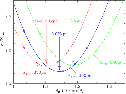
Figure 12: Figure-of-merit $\chi^{2}$ as a function of gas column density $N_{\rm H}^{\rm ISM}$. All our models favor an interstellar column density $N_{\rm H}^{\rm ISM}\approx 1.1-1.2\times 10^{21}\,{\rm cm}^{-2}$ toward Nova Cygni 1992, and $E(B-V)\approx 0.19-0.21$ mag.

Fig. 12 shows $\chi^{2}$ as a function of $N_{\rm H}^{\rm ISM}$ for three exponential density laws. For $z_{1/2}=300\,{\rm pc}$, $\chi^{2}$ is minimized for column density $N_{\rm H}^{\rm ISM}\approx 1.15\times 10^{21}\,{\rm cm}^{-2}$, corresponding to a distance $D\approx 2100\,{\rm pc}$. This model is shown in Figs. 10 and 11 by the solid line. At shorter distances $N_{\rm H}^{\rm ISM}$ is smaller and the model halo is systematically too weak, while for larger distances $N_{\rm H}^{\rm ISM}$ is larger and the model halo is sytematically too strong. The best-fit model still shows systematic discrepancies with the observations – it can be seen from Fig. 11 that the model tends to overpredict the halo intensity for 200–500″ for $t\leq 511\,{\rm d}$, and underpredicts the halo intensity for 50–100″ at all times – but the model halo profiles are in generally good agreement ($\pm\lesssim 40\%$) with the data at all epochs.

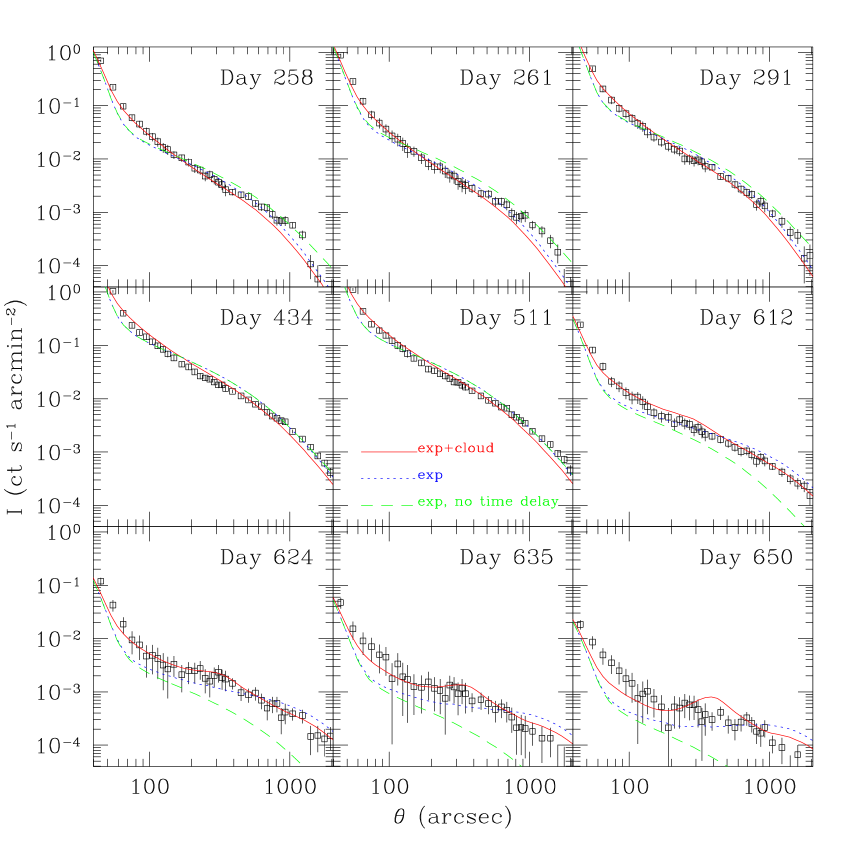
Figure 13: Effect of time delays and of adding a cloud close to the nova: Same as Fig. 11 but showing $D=2.1$ kpc model (dotted line) with same model calculated neglecting time delay effects (dashed line). At early times ($t\leq 291\,{\rm d}$) the effect of time delay is to lower the intensity at large angles; at late times (lower panel) the effect of time delay is to increase the halo intensity at large angles. A “cloud + exponential” model, also for $D=2.1$ kpc, with 70% of dust in the exponential distribution and 30% in a cloud at $y=r/D=0.95$ is shown by the solid line (see also Figs. 14 & 15 and §6.4)

Fig. 12 shows that exponential density laws with different values of $z_{1/2}$ are nearly degenerate: the best-fit distance in each case corresponds to the distance at which the column density $N_{\rm H}(D)\approx 1.15\times 10^{21}\,{\rm cm}^{-2}$, or $D\approx 2100(z_{1/2}/300\,{\rm pc})\,{\rm pc}$. For a steady source these solutions would in fact be perfectly degenerate – the difference between models with the same $N_{\rm H}^{\rm ISM}$ but different $z_{1/2}$ is due to the variability of the source and the different time delays for models with different $D$. The $\chi^{2}$ curves for the 3 different exponential distributions do differ slightly, but evidently the differences in time delay have a relatively small effect on the overall $\chi^{2}$. This is because the effect of time delays on the halos is only prominent at late times when the lightcurve is declining and at large angles where the fluxes are close to the level of the background (see Fig. 13).

Fig. 13 shows X-ray halos at each epoch for our standard model, as well as the results for the same model but with time delays set to zero (e.g., infinite speed of light). Time delay effects are minimal at days 434 and 511 because the light curve (Fig. 2) is relatively constant for $\gtrsim$50 days prior to those two epochs; at earlier epochs ($t\leq 291\,{\rm d}$) the effect of time delay is to reduce the intensity at large angles, and at $t\geq 612\,{\rm d}$ the effect of time delay is to increase the intensity at large angles.

6.3 Reddening

Our modelling of the X-ray halos favors a column density $N_{\rm H}^{\rm ISM}\approx 1.15\times 10^{21}\,{\rm cm}^{-2}$ in order to get the overall halo intensity correct; this column of gas and dust corresponds to a reddening $E(B-V)\approx 0.20$ mag. How does this compare to other reddening estimates?

Barger et al. (1993) measured the H$\alpha$/H$\beta$ intensity ratio at different times. The ratio declined with time, presumably due to the nebula becoming optically thin in the Balmer lines. The last measurement reported by Barger et al. ($t=450\,{\rm d}$ after optical maximum), was $I({\rm H}\alpha)/I({\rm H}\beta)=3.47$; Mathis et al. (1995) make a reasonable extrapolation to an asymptotic value $3.31$, from which they estimate $E(B-V)=0.19$ mag. If the nebula is optically thick in the Balmer lines, radiative transfer effects can lead to an increase in the H$\alpha$/H$\beta$ ratio relative to the “case B recombination” value which is assumed; this would cause $E(B-V)$ to be overestimated. Similarly, at high densities there can be $n=2\rightarrow 3$ collisional excitation, which would again increase H$\alpha$ emission and lead to overestimation of $E(B-V)$. Thus the H$\alpha$/H$\beta$ estimate of $E(B-V)$ should be regarded as an upper bound. Since the H$\alpha$/H$\beta$ estimate of $E(B-V)$ is in agreement with our estimate, it appears that radiative trapping effects do not appreciably affect the H$\alpha$/H$\beta$ ratio at $t\gtrsim 450\,{\rm d}$.

Austin et al. (1996) estimate $E(B-V)=0.40\pm 0.07$ using the He II 1640/4686 line ratio, and $0.38\pm 0.07$ using the [Ne IV] 1602/4724 line ratio. In principle these line ratios should be reliable reddening indicators. However, the He II and [Ne IV] reddening estimates both rely on IUE photometry in the 1600-1640Å range, and we note that the He II 1640/4686 and [Ne IV] 1602/4724 ratios measured by Austin et al. at 5 epochs are strongly correlated, which may indicate calibration errors in the IUE spectrophotometry.

If the interstellar gas column on the sightline to the nova substantially exceeds $1.15\times 10^{21}\,{\rm cm}^{-2}$ and the true reddening significantly exceeds $0.20$ mag, the WD01 dust model will be disfavored: if the column density of interstellar dust and gas is appreciably increased, the predicted halo intensities become too large at most angles and most epochs, and the goodness-of-fit suffers (see Fig. 12). We conclude that the WD01 dust model is incompatible with $E(B-V)\gtrsim 0.3$ in smoothly-distributed dust toward the nova. If $E(B-V)$ is indeed as large as 0.36 (the value recommended by Austin et al.) then either an appreciable fraction of the reddening must be contributed by dust which is located close to the nova (e.g., dust associated with the nova, or interstellar dust within $\sim$50 pc of the nova) which would contribute only to very small halo angles, and would be indistinguishable from the instrumental point spread function) or the WD01 model must be rejected. However, it seems most likely that the reddening is close to $E(B-V)\approx 0.19$ mag, the value obtained from the H$\alpha$/H$\beta$ ratio.

6.4 Dust Distribution Along the Line-of-Sight

The profile of the scattering halo depends on the distribution of dust along the line of sight (e.g., Predehl & Klose 1996). So far we have investigated smooth exponential models. Other smooth distributions, such as gaussian or $\rm sech^{2}(z)$ models, do not change the halos significantly, as long as the intervening H I column remains close to $1.15\times 10^{21}\>{\rm cm^{-2}}$ (this might require the nova to be at a different distance). However, since the total reddening to the nova appears to be just $E(B-V)\approx 0.19$ mag, it would not be implausible for much of this to be contributed mainly by one or two diffuse clouds. In Fig. 14 we show models where the same column density of dust is located in a single cloud located at $y=0.10$, $0.25$, $0.5$, $0.75$, or $0.90$ of the distance to the nova. We see that the halo profile is quite sensitive to the location of the dust along the line of sight: at $\theta=100$″, for example, the halo intensity in the $y=0.10$ case is only 6% of the intensity for the $y=0.90$ case. For a fixed halo angle, there are three separate effects as the dust cloud is moved from small $y$ to large $y$:

1. The inverse square law causes the intensity of the radiation illuminating the dust grains to increase. This acts to increase the surface brightness of the dust cloud.

2. The required scattering angle ${\Theta_{s}}$ increases [see eq. (23) and (24)]. Since $d\sigma/d\Omega$ tends to decrease for increasing ${\Theta_{s}}$, this acts to reduce the scattered intensity.

3. The time delay $\delta t_{1}$ increases as $y$ increases. For $y=0.25$, $\delta t_{1}=9.4\,{\rm d}(D/2.0\,{\rm kpc})(\theta/1000\arcsec)^{2}$, while for $y=0.75$, $\delta t_{1}=84.0\,{\rm d}(D/2.0\,{\rm kpc})(\theta/1000\arcsec)^{2}$. At times when the nova light curve is rising (e.g., day 291) this leads to weakening of the halo at large angles $\theta$ as $y$ is increased.

At small halo angles, the near-constancy of $d\sigma/d\Omega$ at small ${\Theta_{s}}$ (see Fig. 8) causes the first effect to dominate, so the halo intensity increases as $x$ increases (e.g., at 100″, the halo is $\sim$5 times brighter for $y=0.75$ vs. 0.25). At large halo angles, the rapid decline in $d\sigma/d\Omega$ at large ${\Theta_{s}}$ also becomes important, as does the time delay if the lightcurve is rising or falling.

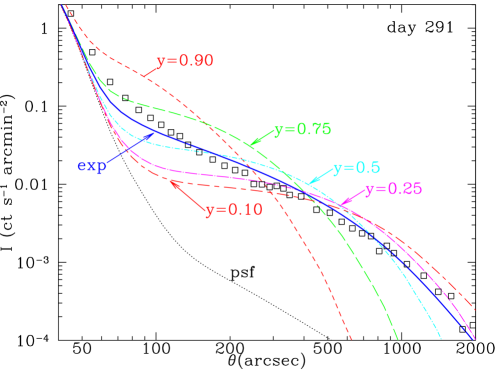
Figure 14: Comparison of the X-ray halo produced by smooth exponentially-distributed dust with $z_{1/2}=300\,{\rm pc}$ and the nova at $D=2.1\,{\rm kpc}$, with models with the same nova distance $D$ and column density $N_{\rm H}$ but in a single cloud at $y=r/D=0.1$, 0.25, 0.5, 0.75, and 0.90.

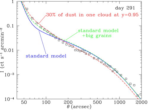
Figure 15: Halo calculated for nova at $D=2.1\,{\rm kpc}$ and (1) standard dust in an exponential distribution (solid line) (2) standard dust plus additional equal mass in large grains with $a=2.0\micron$ in an exponential distribution (dashed line) (3) standard dust, with 70% of dust in an exponential distribution and 30% in a cloud at $y=r/D=0.95$.

In Fig. 15 we show a model where the total column density to the nova is held at $1.15\times 10^{21}\,{\rm cm}^{-2}$, but 30% of this is concentrated in a single “cloud” at $y=0.95$, with the remaining 70% of the dust in an exponential distribution with $z_{1/2}=300\,{\rm pc}$. The agreement between model and observation is excellent. We see that the dust in the cloud near the nova raises the halo intensity at $\theta\lesssim 150\arcsec$, in accord with observations, and removing 30% of the dust from the general exponential distribution acts to lower the intensity at 200–500″, where the model was previously somewhat above the observed halo. We show the above “cloud + exponential” model for all epochs in Fig. 13. At each time, agreement with the data is improved relative to the best smooth model, and is in general excellent. Note that this model is not necessarily the optimum “cloud + exponential” model. In addition to raising the inner and lowering the outer halo, the clumpiness in the distribution imprints structure into the late-time (declining light curve) halos at larger angles (see Fig. 13).

Unfortunately, we have little way of determining the actual distribution of the gas towards the nova, since the nova’s location at $l=89.1^{\circ}$ renders radial velocities unusable for determinations of distances within $\sim$ 1 or 2 kpc. In view of these uncertainties, we conclude that the observed X-ray scattering halo appears to be consistent, within the uncertainties, with the WD01 dust model.

6.5 Very Large Grains?

From Fig. 8 we see that for the WD01 dust model, the X-ray scattering is dominated by the grains with radii $0.1\micron\lesssim a\lesssim 0.4\micron$. Grains larger than $0.4\micron$ contribute less than 20% of the scattering even at small scattering angles ${\Theta_{s}}\lesssim 100$″, and less than 1% at scattering angles ${\Theta_{s}}\gtrsim 1000$″.

A recent paper by Witt et al. (2001) has argued that the observed X-ray halo around Nova Cygni 1992 requires that the dust grain size distribution include significant mass in large dust grains. Witt et al. calculated the dust scattering halo at $t=291\,{\rm d}$ for a monochromatic $h\nu=450\,{\rm eV}$ steady point source. They assumed $N_{\rm H}=2.1\times 10^{21}\,{\rm cm}^{-2}$, and found that a conventional “MRN” ($dn/da\propto a^{-3.5}$) size distribution for $a<0.25\micron$ (Mathis, Rumpl, & Nordsieck 1977), with the dust distributed uniformly along the line-of-sight, reproduced the observed halo intensity at $\theta=100\arcsec$, but overpredicted the halo intensity by a factor $\sim$2 for 300 – 800″; Witt et al. did not consider halo angles larger than 800″. In order to suppress the scattering at large angles, while maintaining the observed halo intensity at small angles, they favored size distributions with the dust mass shifted into larger grains. However, the modifications to the grain size distribution proposed by Witt et al. are inconsistent with the average optical and ultraviolet extinction curve for the Milky Way, and there is no reason to assume that this particular sightline has an anomalous extinction law. It is our contention that the excess scattering at 300–800″ found by Witt et al. is due primarily to assuming too much dust on the line-of-sight – our preferred models have $N_{\rm H}\approx 1.15\times 10^{21}\,{\rm cm}^{-2}$, only $\sim 55\%$ of the $2.1\times 10^{21}\,{\rm cm}^{-2}$ column assumed by Witt et al.

We have taken our best-fitting smooth exponential model – which uses the standard WD01 size distribution which reproduces the standard $R_{V}=3.1$ extinction curve – and modified the grain population by adding very large silicate and carbonaceous dust grains. These grains are arbitrarily given a radius $a=2\micron$, and abundances such that the total silicate mass and total carbonaceous mass is doubled: this trial dust model has 50% of the dust mass in $a=2.0\micron$ grains. Of course this dust model now has twice as much dust mass per unit area toward the nova as the original model.

The results of this model are shown in Fig. 15. The additional dust grains do increase the strength of the scattered halo, but only slightly. The effect is most noticeable in the range 50–100″, where the halo intensity is increased by up to 20%. We see, however, that even with this unreasonably large mass in large grains, this model is not superior to the model discussed in §6.4 where 30% of the dust is assumed to be located in a cloud at a distance $\sim 100\,{\rm pc}$ from the nova. Adding large grains has negligible effect at large angle halos, whereas placing a cloud close to the nova reduces the intensity at large halo angles (since the amount of dust at large distances from the nova is reduced); this reduction appears to improve agreement with the observations. We conclude that while we cannot rule out a population of large grains, these grains would have only a modest effect on the scattered halo, and the observations do not require their presence. A more important and plausible effect on the halo comes from the presence of structure in the ISM.

7 Discussion

Figure 16 shows the importance of various features of the modelling on the intensity of the X-ray halo. The curve labelled “ref” is the single-scattered intensity for a model where the source is radiating steadily at a single energy $h\nu=400\,{\rm eV}$, with uniform dust density between observer and source. Other curves show the effect of including multiple scattering, time delay, and a realistic nova spectrum (same point source count rate), and replacing the uniform dust distribution with an exponential distribution.

• Doubly-scattered photons add $\sim$10% to the intensity at $\theta\approx 600\arcsec$, and $\sim$20% at $\theta\gtrsim 1200$″.

• Changing from a uniform to an exponential dust distribution reduces the intensity for $\theta\lesssim 450$″ (less dust close to the source), and increases the intensity for $\theta\gtrsim 450$″ (more dust far from the source). The increase is $\sim$10% for $\theta>800$″.

• Replacing the monochromatic spectrum with a realistic spectrum reduces the flux at large angles; the adopted $h\nu=400\,{\rm eV}$ is probably slightly low compared to the more realistic spectrum (see Fig. 4), resulting in slightly more large angle scattering than for the more realistic spectrum.

• Since the light curve is rising at day 291, including time delay leads to a reduction in the intensity, particularly for larger halo angles for which the time delays are larger. At 1000″, inclusion of time delay reduces the intensity by $\sim$30%.

Some of these effects increase, others decrease, the intensity. When all are included together, the intensity for day 291 is reduced at angles $>60$″, with a reduction by $\sim$30% at 1000″.

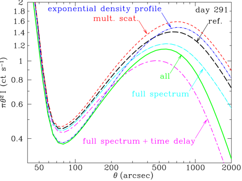
Figure 16: $\pi\theta^{2}I$ for reference model: $h\nu=400\,{\rm eV}$, uniformly-distributed dust. single scattering only, time delay neglected (curve labelled “ref”). Other curves show effect of adding multiple scattering, changing from monochromatic to realistic nova spectrum; including effects of time delay for scattered photons, for $D=2.1$kpc; and changing from a uniform density to exponential density profile with $z_{1/2}=300$pc. Curve labelled “all” is exponential density model with full spectrum, multiple scattering, and time delay.

For smoothly-distributed dust and a standard dust-to-gas ratio, our modelling strongly favors a column density $N_{\rm H}^{\rm ISM}\approx 1.15\times 10^{21}\,{\rm cm}^{-2}$ between us and the nova; this is only $\sim$50% of the estimated total gas column in this direction. This means that the nova must be close enough to have $\sim$50% of the column density beyond it. For the exponential distribution (eq. 4), this places it at a distance $\sim 2.1(z_{1/2}/300\,{\rm pc})\,{\rm kpc}$. Since the actual variation of gas density as a function of height is not well known, and since much of the gas and dust is likely to be contributed by discrete clouds, it is possible for the nova distance to be as large as $2.5\,{\rm kpc}$ and still have $\sim$50% of the gas and dust beyond the nova.

Most estimates of the reddening to the nova have been larger than the value $E(B-V)=0.20$ mag which we favor. Austin et al. took the weighted mean of 5 different methods, and obtained $E(B-V)=0.36\pm 0.04$ mag. Our model with $E(B-V)=0.20$ mag has good overall agreement with the observed halo intensities, but an increase in $E(B-V)$ to 0.36 would result in halo intensities almost twice as strong as observed. If the reddening were shown to be $E(B-V)\gtrsim 0.3$ toward Nova Cygni 1992, this would rule out the WD01 dust grain model which we have used here if the dust is smoothly distributed. However, we note that the reddening estimated from the Balmer decrement at late times is consistent with our estimate.

Furthermore, we show that a plausible modification of the spatial distribution of the dust can produce good agreement between the observed and calculated halos: if $\sim 30\%$ of the dust (i.e., $E(B-V)=0.06$) is located in a “cloud” within $\sim 100\,{\rm pc}$ of the nova, the calculated scattering halo is in good agreement with observation. Since such a spatial distribution is not improbable, the observed X-ray halo around Nova Cygni 1992 does not require the existence of a population of large grains. Recent observations by Chandra of the scattered halo around GX 13+1 also do not support an additional population of large grains (Smith et al. 2002).

While we have shown that the WD01 dust model is generally consistent with observations of Nova Cygni 1992, this conclusion would be overturned if the larger estimates of the reddening prove to be correct. Unfortunately, Nova Cygni 1992 is a less-than-ideal test of a dust model: as we have seen, there is uncertainty regarding the value of the reddening $E(B-V)$ (i.e., the total amount of dust); in addition, there is uncertainty regarding the distribution of gas and dust along the sightline to Nova Cygni 1992 – it was plausible to consider that $\sim$30% of the dust might be contributed by a cloud $\sim$100pc from the nova.

The ideal way to study scattering by interstellar dust is to employ an X-ray source well outside the galactic plane, so that most of the dust contributing to the scattering is at $y\lesssim 0.1$, in which case the halo angle $\theta$ and scattering angle $\Theta_{s}$ are nearly the same for single-scattering. An extragalactic source would be ideal for this purpose. In this case, uncertainties regarding the precise location of the dust in the Galactic disk are unimportant (i.e., dust at $y=0$ and dust at $y=0.001$ produce virtually identical halos). We can hope that the great sensitivity of Chandra and XMM may make feasible observations of such out-of-plane sources. Alternatively, a source located in the galactic plane at $15^{\circ}\lesssim|l|\lesssim 75^{\circ}$ would allow HI or CO observations, or optical absorption line spectroscopy, to locate the absorbing material using galactic rotation.

The higher angular resolution of Chandra may allow observations at smaller halo angles, and the improved energy resolution will allow study of the energy spectrum of the scattered halo.

8 Summary

The principal results of this paper are as follows:

1. We model the X-ray spectrum and light curve of Nova Cygni 1992 using the two-component model of Balman et al. (1998): optically-thin thermal plasma plus a O-Ne enhanced white dwarf atmosphere.

2. We present the formalism for calculating X-ray scattering halos including multiple scattering. Time delay is treated exactly for single scattering and approximately for multiple scattering.

3. We calculate the X-ray halo for Nova Cygni 1992, using the WD01 dust model, consisting of a mixture of amorphous silicate grains and carbonaceous/PAH grains. We compare the calculated X-ray halo with ROSAT PSPC imaging of the halo plus point source at 9 epochs.

4. If the dust toward the nova is smoothly distributed (we consider an exponential density law as an example) we find that the WD01 dust model can quantitatively reproduce the observed halo intensity and angular profile provided the reddening $E(B-V)\approx 0.20$ mag, This is consistent with the value of $E(B-V)\approx 0.19$ mag inferred from the observed H$\alpha$/H$\beta$ emission line ratio at late times.

5. If $E(B-V)\approx 0.20$ mag, then the good agreement between the halo calculated for the WD01 grain model and observations of Nova Cygni 1992 contradicts previous claims that the dust toward Nova Cygni 1992 had to be either highly porous (Mathis et al. 1995) or include a substantial population of very large ($a\gtrsim 1\micron$) dust grains (Witt et al. 2001).

6. Improved agreement between model and observation is obtained if $\sim 30\%$ of the dust is located in a cloud $\sim 100\,{\rm pc}$ from the nova.

7. The effects of time delays on the scattered halos depend on the distance to the source, which thus provides a method for distance determination to non-steady sources. The time delay of the halo relative to the nova is clearly visible at late times when the nova is in decline. The use of time-delay to determine the distance to Nova Cygni 1992 is discussed elsewhere (Draine & Tan 2003).

8. It is hoped that future X-ray imaging by Chandra, XMM, or other telescopes will characterize the X-ray scattering halos around point sources where the dust column can be reliably estimated, and where there is information constraining the distribution of dust along the line of sight. Extragalactic X-ray point sources are ideal for this purpose. As we have shown here, such observations are capable of strongly testing models for interstellar dust.

References

- (1) Allende Prieto, C., Lambert, D.L., & Asplund, M. 2002a, ApJ, 556, L63
- (2) Allende Prieto, C., Lambert, D.L., & Asplund, M. 2002b, ApJ, 573, L137
- (3) Asplund, M. 2000, AA, 359, 755
- (4) Austin, S.J., Wagner, R.M., Starfield, S., Shore, S.N., Sonneborn, G., & Bertram, R. 1996, AJ, 111, 869
- (5) Balman, S., Krautter, J., & Ögelman, H. 1998, ApJ, 499, 395
- (6) Barger, A.J., Gallagher, J.S. III, Bjorkman, K.S., Johansen, K.A., & Nordsieck, K.H. 1993, ApJ, 419, L85
- (7) Binney, J., & Merrifield, M. 1998, Galactic Astronomy (Princeton: Princeton Univ. Press)
- (8) Boese, F.G. 2000, A&AS, 141, 507
- (9) Catura, R.C. 1983, ApJ, 275, 645
- (10) Chochol, D., Grygar, J., Pribulla, T., Komz̆ík, R., Hric, L., & Elkin, V. 1997, A&A, 318, 908
- (11) Clark, G.W., Woo, J.W., & Nagase, F. 1994, ApJ, 422, 336
- (12) Draine, B.T. 2003a, ARAA, 41, 000
- (13) Draine, B.T. 2003b, submitted to ApJ. astro-ph/0304060
- (14) Draine, B.T., & Bahcall, J.N. 1981, ApJ, 250, 579
- (15) Draine, B.T., & Tan, J.C. 2003, in preparation
- (16) Grevesse, N., & Sauval, A.J. 1998, Space Sci. Rev., 85, 161
- (17) Hartmann, D., & Burton, W.B. 1997, Atlas of galactic neutral hydrogen (New York: Cambridge University Press)
- (18) Hayakawa, S. 1973, in Interstellar Dust and Related Topics, IAU Symposium No. 52, ed. J.M. Greenberg & H.C. van de Hulst (Dordrecht: Reidel), p. 283
- (19) Krautter, J., Ögelman, H., Starrfield, S., Wichmann, R., & Pfeffermann, E. 1996, ApJ, 456, 788
- (20) Li, A., & Draine, B.T. 2001, ApJ, 554, 778
- (21) Li, A., & Draine, B.T. 2002, ApJ, 572, 000
- (22) MacDonald, J., & Vennes, S. 1991, ApJ, 373, L51
- (23) Martin, P.G. 1970, MNRAS, 149, 221
- (24) Mathis, J.S., Cohen, D., Finley, J.P., & Krautter, J. 1995, ApJ, 449, 320
- (25) Mathis, J.S., & Lee, C.-W. 1991, ApJ, 376, 490
- (26) Mathis, J.S., Rumpl, W., & Nordsieck, K.H. 1977, ApJ, 217, 425
- (27) Mauche, C.W., & Gorenstein, P. 1986, ApJ, 302, 371
- (28) Mitsuda, K., Takeshima, T, Kii, T., & Kawai, N. 1990, ApJ, 353, 480
- (29) Overbeck, J.W. 1965, ApJ, 141, 864
- (30) Paresce, F. 1994, A&A, 282, L13
- (31) Predehl, P., Burwitz, V., Paerels, F., & Trümper, J. 2000, A&A, 357, L25
- Predehl & Klose (1996) Predehl, P., & Klose, S. 1996, A&A, 306, 283
- Predehl & Schmitt (1995) Predehl, P., & Schmitt, J.H.M.M. 1995, A&A, 293, 889
- (34) Raymond, J., & Smith, B.H. 1977, ApJS, 35, 419
- (35) Shore, S.N., Schwarz, G., Bond, H.E., Downes, R.A., Starrfield, S., Evans, A., Gehrz, R.D., Hauschildt, P.H., Krautter, J., & Woodward, C.E. 2003, AJ, 125, 1507
- (36) Smith, R.K., & Dwek, E. 1998, ApJ, 503, 831
- (37) Smith,R.K., Edgar, R.J., & Shafer, R.A. 2002, ApJ, 581, 562
- (38) Snowden, McCammon, Burrows, & Mendenhall 1994, ApJ, 424, 714
- (39) Trümper, J., & Schönfelder, V. 1973, A&A, 25, 445
- (40) van de Hulst, H.C. 1957, Light Scattering by Small Particles, (New York: Wiley)
- (41) Verner, D.A. 1996, Fortran code phfit2.f obtained from ftp://gradj.pa.uky.edu//dima//photo//phfit2.f
- (42) Verner, D.A., Ferland, G.J., Korista, K.T., & Yakovlev, D.G. 1996, ApJ, 465, 487
- (43) Verner, D.A., & Yakovlev, D.G. 1995, A&AS, 109, 125
- (44) Weingartner, J.C., & Draine, B.T. 2001, ApJ, 548, 296 (WD01)
- Wiscombe (1980) Wiscombe, W.J. 1980, Appl. Opt., 19, 1505
- Wiscombe (1996) Wiscombe, W.J. 1996, NCAR Technical Note NCAR/TN-140+STR, ftp://climate.gsfc.nasa.gov/pub/wiscombe/Single-Scatt/Homogen_Sphere/ Exact_Mie/NCARMieReport.pdf
- (47) Witt, A.N., Smith, R.K., & Dwek, E. 2001, ApJ, 550, L201
- (48) Woo, J.W., Clark, G.W., Day, C.S.R., Nagase, F., & Takeshima, T. 1994, ApJ, 436, L5
- (49) Woodward, C.E., Gehrz, R.D., Jones, T.J., Lawrence, G.F., & Skrutskie, M.F. 1997, ApJ, 477, 827