Monocular Measurement of the Spectrum of UHE Cosmic Rays by the FADC Detector of the HiRes Experiment

Abstract

We have measured the spectrum of UHE cosmic rays using the Flash ADC (FADC) detector (called HiRes-II) of the High Resolution Fly’s Eye experiment running in monocular mode. We describe in detail the data analysis, development of the Monte Carlo simulation program, and results. We also describe the results of the HiRes-I detector. We present our measured spectra and compare them with a model incorporating galactic and extragalactic cosmic rays. Our combined spectra provide strong evidence for the existence of the spectral feature known as the “ankle.”

1 Introduction

The aim of the High Resolution Fly’s Eye (HiRes) experiment is to study the highest energy cosmic rays using the atmospheric fluorescence technique. In this paper we describe the data collection, analysis, and Monte Carlo calculations used to measure the cosmic ray spectrum with the HiRes experiment’s FADC detector, HiRes-II. We also describe the analysis performed on the data collected by the HiRes-I detector and present the two monocular spectra, covering an energy range from $2\times 10^{17}$ eV to over $10^{20}$ eV. We perform a statistical test of the combined spectra which gives strong evidence for the presence of the spectral feature known as the “ankle.” We conclude with a fit of our data to a toy model incorporating galactic and extragalactic cosmic ray sources.

The acceleration of cosmic rays to ultra high energies is thought to occur in large regions of high magnetic fields expanding at relativistic velocities[1]. Such structures are rare in the neighborhood of the Milky Way galaxy and many of the cosmic rays that we observe may have traveled cosmological distances to reach us. Hence they are probes of conditions in some of the most violent and interesting objects in the universe.

The highest energy particles from terrestrial particle accelerators have energy $1\times 10^{12}$ eV, so the cosmic rays we observe have energies at least five orders of magnitude higher. Since we observe showers in the atmosphere initiated by the cosmic ray particles, we are sensitive to their composition and to the details of their interactions with matter.

Interactions of high energy protons, traveling large distances across the universe, with photons of the cosmic microwave background radiation can excite nucleon resonances which decay to a nucleon plus a $\pi$ meson. This is an important energy loss mechanism for the cosmic rays, and results in the Greisen-Zatsepin-Kuzmin (GZK) cutoff[2], which is often stated as: cosmic rays traveling more than 50 Mpc should have a maximum energy of $6\times 10^{19}$ eV, if sources are uniformly distributed. Several events above this energy have been seen by previous experiments[3, 4, 5], but statistics are low and it is crucial to search for more events above the GZK cutoff.

The spectrum of cosmic rays has few distinguishing features. It consists of regions of power law behavior with breaks in the power law index. There is a steepening from E^-2.7 to E^-3.0 at about $3\times 10^{15}$ eV (called the knee)[6] and a hardening at higher energy (called the ankle). The Fly’s Eye experiment[4], observing in stereo mode, saw a second knee (or steepening of the spectrum) at $4\times 10^{17}$ eV and the ankle at $3\times 10^{18}$ eV. The second knee has also been observed by the Akeno experiment[7]. The Haverah Park experiment[8] observed the ankle at about $4\times 10^{18}$ eV. The Yakutsk experiment[9] has seen both the second knee and the ankle. The AGASA experiment[5], which has a large enough aperture to collect events with energies of $10^{20}$ eV, observes a higher flux than Fly’s Eye, and the ankle at $1\times 10^{19}$ eV. They observe a dip at the GZK threshold, but their spectrum then recovers at higher energies.

The atmospheric fluorescence technique has its basis in the fact that, on average, approximately five UV fluorescence photons[16] will be emitted when a minimum ionizing particle of charge $e$ passes through one meter of air. In HiRes, we detect these photons and reconstruct the development of cosmic ray air showers. We collect the fluorescence light with spherical mirrors of area 5.1 m², and focus it on a $16\times 16$ array of photomultiplier tubes, each of which looks at about one degree of the sky. We record the integrated pulse height and trigger time information from each tube, and can reconstruct the geometry of the air shower and the energy of the primary cosmic ray that initiated it.

HiRes consists of two detector sites located on desert hilltops on the U. S. Army’s Dugway Proving Ground in west central Utah. The first site, called HiRes-I, consists of 22 detectors that look between 3 and 17 degrees in elevation and almost 360 degrees in azimuthal angle[10]. This detector uses an integrating ADC readout system which records the photomultiplier tubes’ pulse height and time information.

The second site, called HiRes-II and located 12.6 km away, consists of 42 detectors looking between 3 and 31 degrees in elevation, and has a Flash ADC (FADC) system to save pulse height and time information from its phototubes[11]. The sampling period of the FADC electronics is 100 ns. Cosmic ray air showers with energies near $10^{20}$ eV and occurring within a radius of 35 km, can trigger the HiRes detectors and can be reliably reconstructed.

The two detector sites are designed to observe cosmic ray showers steroscopically. This stereo mode observation gives us the best geometric resolution, about 0.6 degrees in pointing angle and 100 m in distance to the shower. In this mode we make two measurements of the particle’s energy and thus can make an empirical determination of our energy resolution. The limitation of stereo mode is a geometrically imposed lower energy threshold of $10^{18}$ eV. At this energy the events lie halfway between the two detectors, about 6 km from each.

In monocular mode, the HiRes-II detector can observe events much closer and dimmer than is possible in stereo mode; the energy threshold for this mode is about $2\times 10^{17}$ eV. The geometric resolution is still good: about 5 degrees in pointing angle and 300 m in distance. In this paper we describe the operation and data analysis for the HiRes-II detector, briefly describe the differences between HiRes-I and HiRes-II, and present the monocular spectra of the two detectors.

2 Calibration Issues

There are two important calibration issues in HiRes: the first is the absolute calibration of the phototubes’ pulse heights in photons. This is accomplished by carrying a standard light source to each of our detectors and illuminating the phototubes with it[12]. This source is absolutely calibrated using NIST calibrated photodiodes to about 10% accuracy and this uncertainty appears in our energy measurements.

Since the atmosphere is both our calorimeter and the medium through which we look, we must correct for the way it absorbs and scatters fluorescence light. The determination of the characteristics of the atmosphere is our second important calibration. Both the molecular and aerosol components of the atmosphere contribute to the scattering. The molecular component is well known, but we must measure the aerosol component’s contribution. Two steerable YAG lasers, one at each site and operating at wavelength $\lambda=355$ nm, are used for the aerosol calibration. The scattered light from the laser at one detector is observed by the other detector. In this way we measure the scattering length, angular distribution of the scattering cross section, and vertical aerosol optical depth (VAOD) of aerosol particles in the atmosphere[13]. The aerosol scale height is obtained from the product of horizontal extinction length at ground level times the VAOD.

Figure 1 shows the amount of light detected as a function of scattering angle for one of these laser events. This shot was fired horizontally from the HiRes-II site and passed within 400 meters of the HiRes-I detector. This geometry allows us to observe a wide range of scattering angles. The filled squares show the data, and the open squares are a fit to this data using a four parameter model of the aerosol extinction length and angular distribution. The forward peak seen in this figure is characteristic of aerosol scattering and the relatively flat distribution at backward scattering angles is characteristic of molecular scattering. The horizontal aerosol extinction length measured from this laser event is 23 km. For comparison, the horizontal molecular extinction length at this same wavelength (355 nm) is 18 km. These extinction lengths correspond approximately to the average of atmospheric conditions during our observations at Dugway.

Figure 1: Intensity of laser light scattered into the HiRes-I detector plotted against the scattering angle of the light. The filled squares are the data and the open squares are a four-parameter fit to the data. The discontinuity between 100 and 116 degrees is due to the parallax of a mirror farther from the laser track.

We perform the laser measurement of atmospheric conditions hourly during data collection. For the analysis reported here the average of hourly aerosol scattering lengths and scale heights were used. Since the data has good statistics and the events were collected evenly over the period in question, they will be well described by the average atmospheric conditions [13], which were: aerosol scattering length of $22\pm 2$ km and scale height of 1.1 km. The RMS of the scale height distribution was 0.4 km, and the systematic uncertainty was smaller than this.

3 Data Analysis

The FADC data acquisition system records a 10 $\mu$s long series of ADC samples (100 samples total) for each active photomultiplier tube (PMT) in an event. The starting time of the series is chosen to have the peak of the signal pulse in the middle of the sample.

The first step in the analysis of the data consists of pattern recognition to choose which hit tubes were on the track of the cosmic ray event. As a cosmic ray shower propagates down through the atmosphere, the mirrors collect the generated photons and focus them onto the arrays of phototubes. The image moves across the array illuminating one or more tubes at a time. Therefore, tubes on the cosmic ray track are near each other in two ways: spatially and temporally. Phototubes must be near each other in both position and time to be included in the track. The top two quarters of Figure 2 show the picture of an event, where one can see that the tubes on the shower form a line. The lower left part of this figure is a time plot: a plot of the light arrival times (in FADC time-bin units) on the vertical axis versus the angle of the tube measured along the track. From these plots, it is clear that the tubes related to the air shower can be separated from those firing from random sky fluctuations. The elevation and azimuthal angles of the PMT’s on the track are fit to determine the plane which contains the shower and the detector.

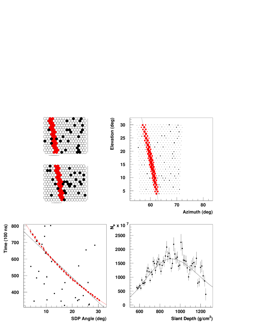
Figure 2: Display of an Event with a Reconstructed Energy of $2.4\times 10^{19}$ eV. The upper left part of this figure shows the two mirrors that triggered for this event. The upper right panel shows the azimuthal vs. elevation angles of triggered tubes, with a fitted shower-detector plane superimposed. The lower left panel shows the time of the tube hits in FADC time slices vs. the angle of the tube measured along the track, with two fits superimposed: a straight line and the result of the time fit. The lower right quarter shows the number of charged particles in the shower as a function of slant depth (in g/cm²), with the fit to the Gaisser-Hillas formula (Eq 2) superimposed.

In a monocular determination of the shower geometry, the angle of the shower within the shower detector plane is determined from the time plot of the active tubes (see the lower left quadrant of Figure 2). One can show that

$$t_{i}=t_{0}+\frac{R_{p}}{c}\tan\left(\frac{\pi-\psi-\chi_{i}}{2}\right)$$ (1)

where $t_{i}$ is the arrival time of light from shower segment $i$, $\chi_{i}$ is the angle in the plane containing the shower and detector from the ground to segment $i$, $t_{0}$ is the earliest possible arrival time, $R_{p}$ is the impact parameter of the shower, and $\psi$ is the angle the shower makes with the ground in the shower-detector plane. The geometry of the shower detector plane is shown in Figure 3. We measure $t_{i}$ and $\chi_{i}$, and need to fit for $t_{0}$, $\psi$ and $R_{p}$. $\psi$ and $R_{p}$ determine the geometry within the shower-detector plane. Since equation 1 is linear in $R_{p}$ and $t_{0}$, we fit for those variables for fixed values of $\psi$ from $5^{\circ}$ to $75^{\circ}$ in $1^{\circ}$ steps. The best geometry is chosen by minimizing $\chi^{2}$, and the uncertainty in $\psi$ from the angles which increase the $\chi^{2}$ by one.

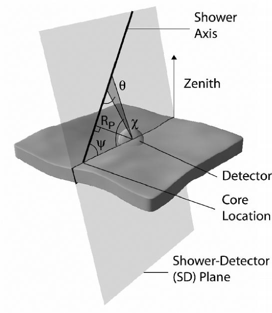
Figure 3: Illustration of monocular reconstruction of the shower geometry, showing the shower-detector plane, the impact parameter, $R_{p}$, and the in-plane angle shower angle, $\psi$.

Once the geometry of the shower is known, we can reconstruct the number of charged particles in the shower as a function of the slant depth of atmosphere through which the shower has passed. To do this, we collect the photoelectrons from tubes on the track into successive time bins, which are multiples of the FADC sampling period. Typically several tubes will contribute to each time bin. Systematic errors in calculating the acceptance of individual tubes tend to be offset by correlated errors in neighboring tubes, reducing the overall uncertainty in the acceptance calculation. We then correct for the sum of the acceptance of all the participating PMT’s and for the quantum efficiency of the phototubes, the mirror reflectivity and the transmission of the HiRes UV filter. This yields the flux of photons striking the mirror.

To convert the photon flux at the detector into the number of charged particles at the observed position of the shower[14], we first correct for the solid angle of the mirror with respect to the shower. We then correct for the amount of light lost due to scattering and absorption in the atmosphere. This includes light scattered by Raleigh scattering from air molecules, Mie scattering from aerosol particles and absorption due to ozone. The first calculation of the attenuation correction is done assuming that all the observed photons come from the fluorescence spectrum given in Bunner[15]. The solid angle and attenuation corrections give the photon flux at the observed portion of the shower. Finally, we calculate the charged particle multiplicity at the shower using the fluorescence yield measurements of Kakimoto et al[16].

The charged particle multiplicity distribution is fit to the Gaisser-Hillas profile function[17]:

$$N(X)=N_{max}(\frac{X-X_{0}}{X_{max}-X_{0}})^{\frac{X_{max}-X_{0}}{\lambda}}\exp(\frac{X_{max}-X}{\lambda}),$$ (2)

where $N(X)$ is the number of charged particles in the shower at slant depth $X$, $N_{max}$ is the number of particles at shower maximum, $X_{max}$ is the slant depth of the maximum, and $\lambda$ is a shower-development parameter. We have seen in previous measurements that the Gaisser-Hillas profile function fits extensive air showers very well[18]. Our fits are very insensitive to $X_{0}$ and $\lambda$ and we fix them at -60 and 70 g/cm², respectively. The $X_{0}$ value is chosen to agree with our fits to Corsika showers (see below).

We calculate the correction for scattered Čerenkov light as follows. We use the fitted Gaisser-Hillas function to simulate the development of the beam of Čerenkov photons accompanying the shower, and calculate the number of these photons scattered into our detector acceptance. The atmospheric attenuation is recalculated for the mixture of fluorescence and scattered Čerenkov photons, and the relative numbers of photoelectrons from fluorescence and Čerenkov sources are found after applying the filter transmission and quantum efficiency corrections using the appropriate spectra. The photoelectrons from Čerenkov photons are subtracted from the signal, and the charged particle multiplicity is recalculated again as described above. This iterative process is continued until stability is achieved. This Čerenkov correction is typically about 15%. The lower right part of Figure 2 shows the development profile of a shower after the correction has been performed, and the Gaisser-Hillas function fit to this profile.

We integrate the final fitted Gaisser-Hillas function over all $X$ and multiply by the average energy loss per particle (2.19 MeV/g/cm²) to determine the visible shower energy. The visible energy is then corrected for energy carried off by unobservable particles[19] to give the total shower energy.

Cuts are applied to select well-reconstructed events and to assure good resolution. The cuts used in the determination of the UHE cosmic ray spectrum are listed below:

• Angular speed $<11^{\circ}\ \mu s^{-1}$

• Selected tubes $\geq 7$

• 0.85 $<$ Tubes/degree $<$ 3.0

• Photoelectrons/degree $>$ 25

• Track length $>7^{\circ}$, or $>10^{\circ}$ for events extending above $17^{\circ}$ elevation

• Zenith angle $<60^{\circ}$

• 150 $<X_{max}<1200{\rm\ g/cm}^{2}$, and is visible in detector

• Average Čerenkov Correction $<$ 60%

• Geometry fit $\chi^{2}$/d.o.f. $<$ 10

• Profile fit $\chi^{2}$/d.o.f. $<$ 10

4 Development of the Monte Carlo Simulation Program

We calculated the aperture of the detector using two Monte Carlo simulation programs. First we generated a library of cosmic ray showers using the programs CORSIKA[20] and QGSJET[21]. We then use events from the library as input to a second program which calculates the response of the detector and writes out simulated events in the same format as the data. Finally, we analyze the Monte Carlo events using the same programs used for the data.

The shower library consists of 200 showers with proton and 200 showers with iron primaries generated for each combination of five fixed primary energies from $10^{16}$ eV to $10^{20}$ eV and three fixed zenith angles of the shower axis with a secant of 1.00, 1.25 and 1.50. Each shower is characterized by its depth of first interaction in the atmosphere, energy, zenith angle, type of primary particle, and the four parameters of a Gaisser-Hillas fit to its profile (the Gaisser-Hillas formula fits CORSIKA + QGSJET showers very well).

When we use these events, we must scale their parameters in energy from the (discrete) energies of the shower library to the continuous energy spectrum we throw in the detector-response Monte Carlo program. Figure 4 shows the energy dependence of the four Gaisser-Hillas parameters. In scaling the parameters of a shower we use the slopes shown in the four parts of this figure. Use of a shower library preserves the event-to-event fluctuations and correlations in the CORSIKA events.

Figure 4: Energy Dependence of Gaisser-Hillas Parameters. The four panels show (clockwise from upper left) the energy dependence of $N_{max},X_{max},\lambda$, and $X_{0}$ for showers at zenith angle of 36.9 degrees.

Since we change the geometry of the showers at random, one CORSIKA shower can be used over and over to create different events. This allows us to generate approximately 30 times as many events per minute with the shower library as we could directly with CORSIKA.

The detector-response program simulates the generation of fluorescence and Čerenkov light by the shower and the operation of the two HiRes detectors, including optics, trigger, electronics, and data acquisition. To generate an event, the program chooses the primary energy and the primary particle type from the spectrum and composition measured in stereoscopic mode by the Fly’s Eye experiment[4]. The zenith angle and distance to the shower are chosen randomly. An event from the shower library bin whose fixed energy and zenith angle are closest to the chosen values is then used to generate the profile of the shower’s development. We scale each of the four Gaisser-Hillas parameters to the thrown energy. The dependence of the Gaisser-Hillas parameters on zenith angle is quite weak, hence we simply use the three bins in zenith angle.

An accurate simulation of fluorescence and Čerenkov light is performed [19], including the shower profile, the average $dE/dx$ for each part of the shower, and atmospheric pressure, the width of the showers, the energy of particles that fall below the Corsika thresholds (we use 0.1 MeV for electrons and photons, 0.3 GeV for hadrons, and 0.7 GeV for muons), calorimetric energy, and the unobserved energy (mostly neutrinos and muons that strike the ground).

Previous publications describe how we calculate fluorescence and Čerenkov light emission, scattering, and transmission[14]. The fluorescence spectrum is taken from Bunner et al.[15], and the overall normalization from Kakimoto et al[16]. The response due to mirror reflectivity, HiRes filter transmission, and phototube quantum efficiency is included. A complete wavelength-dependent calculation is performed for all these effects in 16 wavelength bins between 290 and 410 nm.

To simulate the exact conditions of the experiment, we created a database of parameters that vary from night to night: live time, trigger logic, trigger gains and thresholds, and specific mirrors in operation. Two parameters which vary with time, but which we treated only in an average way, are the sky noise and atmospheric scattering of fluorescence light.

These parameters are read into the detector response programs individually for each event, allowing us to simulate precisely the detector settings recorded during data collection. Direct comparisons of Monte Carlo events and real data, such as those shown below, give us confidence in our detector response programs and prove that we understand our detectors.

The data that went into the comparison plots shown below were recorded by the HiRes-II-detector from 1 December 1999, through 4 May 2000. There are about 2100 events after cuts. The Monte Carlo sample contains about five times as many events. The first two graphs presented here (see Figures 5 and 6) show two basic geometric quantities: the zenith angle distribution and the distance to the shower mean (found by weighting each PMT that was on the track by the number of observed photoelectrons). The upper panels of the graphs show the data as open squares and histograms and the Monte Carlo as filled squares. The data and MC distributions have been normalized to the same area. In the lower panels, the ratio of data divided by MC and a linear fit to this ratio are shown. It can be seen from Figures 5 and 6 that the distributions of these geometric quantities agree very well. Figure 7 shows the $\chi^{2}$ of a linear fit to the time plot (such as is shown in the lower left quadrant of Figure 2). The agreement shows that the experimental resolution is well simulated in the Monte Carlo program.

An important non-geometric quantity is the amount of light that is seen by the detector. It can be characterized by the number of photoelectrons we receive per degree of track length. Figure 8 shows that the amount of light we see with our detectors and the amount of light we generate in our MC programs closely agree with each other. Figure 9 shows a histogram of the reconstructed energy of events.

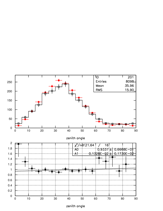
Figure 5: Zenith Angle of Cosmic Ray Showers. In the upper panel the data is shown as open squares and histogram and the Monte Carlo (which has been normalized to the number of data events) is shown as closed squares. The lower panel shows the ratio of data to Monte Carlo events.

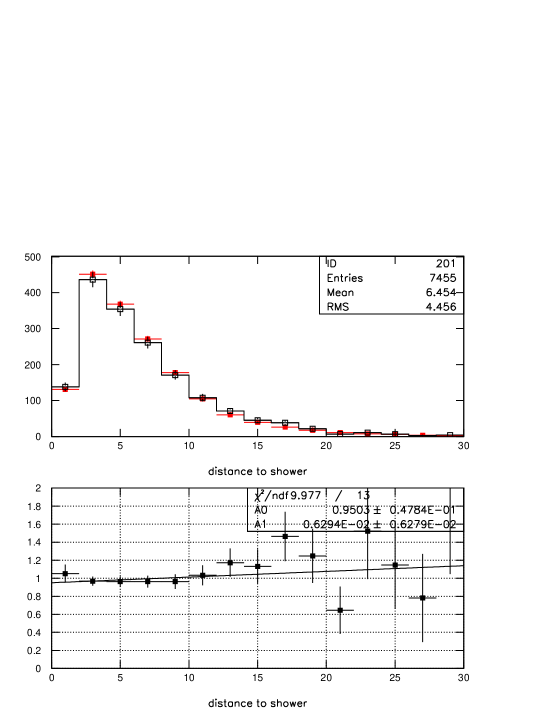
Figure 6: Distance from the Detector to the Shower Mean (weighted by photoelectrons). Again data is shown as open squares and histogram and Monte Carlo as closed squares, and the lower panel shows the data to Monte Carlo ratio.

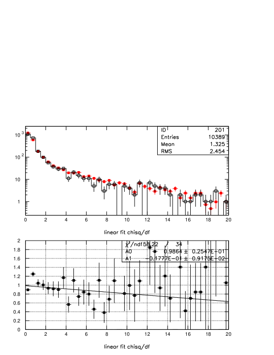
Figure 7: Comparison of data and MC for the $\chi^{2}$ of a linear fit to the time vs angle plot.

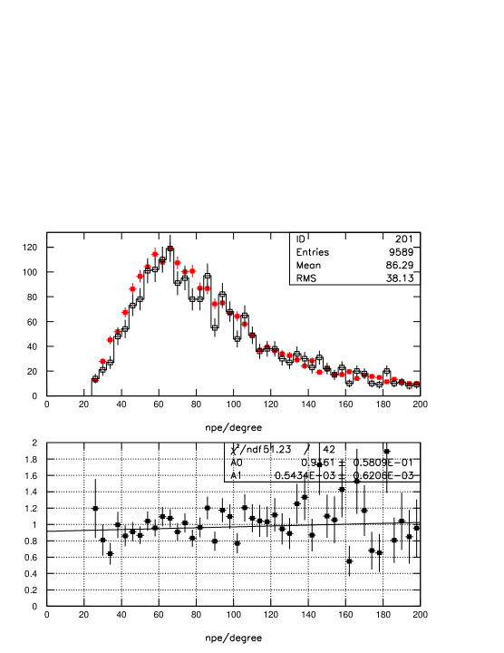
Figure 8: Comparison of data and MC for the photoelectrons per degree of track

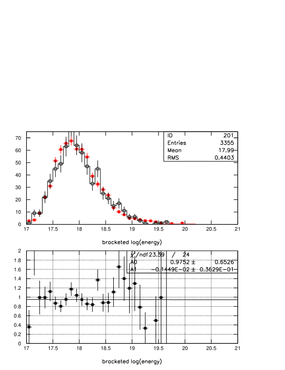
Figure 9: Comparison of data and MC for the reconstructed Energy

The excellent agreement between the data and Monte Carlo simulation in these plots is characteristic of our Monte Carlo as a whole and demonstrates that the Monte Carlo models the data well.

5 The UHE Cosmic Ray Spectrum

Having demonstrated that our MC models the detector accurately, we have confidence in using it to calculate the detector aperture. This aperture is shown in Figure 10.

Figure 10: Monte Carlo calculated aperture of the HiRes-II detector used for this spectrum measurement.

To make an accurate calculation of the flux of cosmic rays it is important to use a continuous Monte Carlo input spectrum in order to take account of the finite energy resolution of the detector. With this in mind, we define the flux, $J(E)$, as follows:

$$J(E)=N_{D}(E)\frac{N_{T}(E)}{N_{A}(E)}\frac{1}{\Delta EA\Omega T}$$ (3)

where $N_{D}(E)$ is the number of data events in energy bin $E$, $N_{T}(E)$ is the number of thrown MC events in energy bin $E$ binned by the thrown energy, $N_{A}(E)$ is the number of accepted MC events in energy bin $E$ binned by the reconstructed energy, $\Delta E$ is the width of energy bin $E$, $A$ is the area into which the MC generated events, $\Omega$ is the solid angle into which the MC generated events, and $T$ is the total running time of the detector. The MC generated events within a 35 km radius of the detector and with zenith angles from 0^∘ to $70^{\circ}$. For the data included in this paper, recorded from 1 December 1999 to 4 May 2000, the detector was live for 144 hours. This includes data only from nights with good weather. This time period represents the first period of stable running for the HiRes-II detector. After this period the trigger was changed considerably, so subsequent data have to be analyzed separately.

An important feature of Equation 3 is that when one has modeled the experimental resolution correctly and put in the correct thrown energy spectrum, $N_{T}(E)$, the ratio $N_{D}(E)/N_{A}(E)$ becomes a constant independent of energy. In this situation, one makes a first order correction for experimental resolution[22]; the spectrum one calculates has the shape of $N_{T}(E)$. The comparisons between data and Monte Carlo (see especially Figures 7 and 9) show that our modeling is accurate.

The measured spectrum, $J(E)$, is shown in Figure 11. The measured spectrum multiplied by $E^{3}$ is shown in Figure 12. For the latter, the average energy of the data events in each bin is used to compute the $E^{3}$ factor.

Panel a of Figure 12) shows the HiRes-II spectrum in comparison with two previous fluorescence experiments, Fly’s Eye[4] (stereo) and HiRes-MIA[23]. The agreement between the three is quite good. Since different methods were used to calibrate the three experiments, one expects slightly different results. The three results are all within the calibration uncertainties of each experiment. Panel b of Figure 12 shows the HiRes-II spectrum in comparison with three ground array experiments, Akeno[7], Haverah Park[8] and Yakutsk[9]. Differences in energy scale calibration between experiments are accentuated by the $E^{3}$ factor.

Figure 11: Flux of UHE Cosmic Rays measured by the HiRes-II detector.

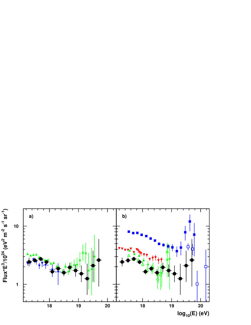
Figure 12: E³ times the HiRes-II UHE Cosmic Ray Flux (filled circles), focusing on the energy region just below the ankle. Panel a) includes the results of other fluorescence experiments: Fly’s Eye Stereo[4] (up triangles) and HiRes/MIA[23] (down triangles). Panel b) includes the results of various ground array experiments: Akeno[7] (down triangles), Haverah Park[8] proton analysis (filled up triangles) and iron analysis (open up triangles), and Yakutsk[9] trigger-500 (closed squares) and trigger-1000 data (open squares).

The Fly’s Eye experiment, in their stereo analysis, observed the ankle feature at $3\times 10^{18}$ eV. To test whether this feature is seen in the HiRes-II data, we fit the HiRes-II spectrum to both a single power law and to a double power law with a floating break point. The single power law fit results in a spectra index, $\gamma=-3.12\pm 0.04$, with a $\chi^{2}=14.1$ for 13 degrees of freedom. The double power law fit results in a spectral index, $\gamma_{1}=-3.16\pm 0.05$ below the break point, $\log_{10}E=18.5\pm 0.4$, and a spectral index, $\gamma_{2}=3.0\pm 0.2$, above the break point. The $\chi^{2}$ for this fit was 12.0 for 11 degrees of freedom. The $\chi^{2}$ was reduced by 2.1 while adding 2 parameters. Since the $\chi^{2}$ did not improve significantly, we cannot claim evidence for the ankle in the HiRes-II monocular data alone.

6 HiRes-I Analysis

In addition to the monocular data collected by the HiRes-II detector, we have a considerable amount of monocular data collected by HiRes-I. In this section we describe the differences between the two detectors and their analyses, and in the next section present both monocular spectra. For a more complete description of the HiRes-I detector and its analysis see references[10] and[24].

The most important differences between the HiRes-I and HiRes-II detectors are the time resolution and the number of mirrors. The HiRes-II time resolution is about a factor of two better than that of HiRes-I, and the one ring of mirrors at HiRes-I means that the tracks are shorter. These factors affect the resolution of the time vs. angle plot (a time plot for HiRes-II is shown is the lower left quadrant of Figure 2). A third difference between the two detectors’ data is that in this paper we are reporting data covering four years of running for HiRes-I (from 29 May 1997 to 7 Feb. 2003) and six months for HiRes-II.

In reconstructing the geometry of tracks seen by the HiRes-I detector, we wish to measure $R_{p}$ and $\psi$ from the curvature in the time plot (a HiRes-II time plot is displayed in the lower left quadrant of Figure 2). But the shorter tracks means the uncertainty in $R_{p}$ and $\psi$ are greater than we would wish for many events. To solve this problem, we add to our fitting procedure a constraint based on the longitudinal energy deposition profile of the event (for a HiRes-II longitudinal profile plot see the lower right quadrant of Figure 2). From previous experiments using fluorescence detectors[18], and from the HiRes-II analysis reported here, we know that the Gaisser-Hillas formula in Equation 2 fits our events very well. While $X_{max}$ varies from event to event and depends logarithmically on the atomic weight of the nucleus and initial energy, the shape of the shower is largely independent of these. Therefore, we use the fact that the shower width does not change with energy or composition to constrain the fit.

The profile-constrained geometry fit proceeds by first calculating a combined $\chi^{2}$ for the time and profile fits. Each phototube on the track makes one contribution to the time fit and one to the profile fit. A map of $\chi^{2}$ is made in six steps in $X_{max}$ and 180 steps in $\psi$. The $X_{max}$ values used are 685, 720, 755, 790, 825, and 960 g/cm². These values span the range of $X_{max}$ values expected for our energy range. The $\psi$ values range from 1 to 180 degrees. For each of the map points, the fit is performed with the Gaisser-Hillas parameter $X_{0}$ fixed to -60 g/cm². In the vicinity of the minimum of the $\chi^{2}$ map a finer search is performed, which includes varying the orientation of the shower-detector plane within bounds of the fired photomultiplier tube apertures. To ensure that the reconstruction process has been accurate, we demand that:

• The Čerenkov light contribution to the observed flux be less than 20%,

• The track length be greater than 7.9 degrees,

• The depth of the first observed point be less than 1000 g/cm²,

• Angular speed $<3.4^{\circ}\ \mu s^{-1}$,

• The average effective mirror area seen by the hit tubes for the event $>0.9$ m²,

• $\psi<120^{\circ}$.

In a Monte Carlo study of the profile-constrained geometry fit, we find that the method works well. However, it introduces a small bias into the reconstructed energy. The bias is 15% at $3\times 10^{18}$ eV and falls to 5% at $3\times 10^{19}$ eV. Figure 13 shows the reconstructed energy divided by the Monte Carlo thrown energy at $3\times 10^{18}$ eV. The bias is evident from the fact that the peak does not occur at 1. Superimposed upon this plot is a similar plot determined from our stereo data. Here the stereo information was used to precisely determine the geometry of the event, but the energy was reconstructed using only information from HiRes-I. Stereo geometry is like the Monte Carlo in that in both cases the geometry is well known. Thus, it is a good test of geometric effects in reconstruction. The two curves agree very well. The shift was parameterized and a correction applied to the data. In Figure 14, the corrected energy from the profile-constrained geometry fit is compared to the energy calculated using stereo geometry.

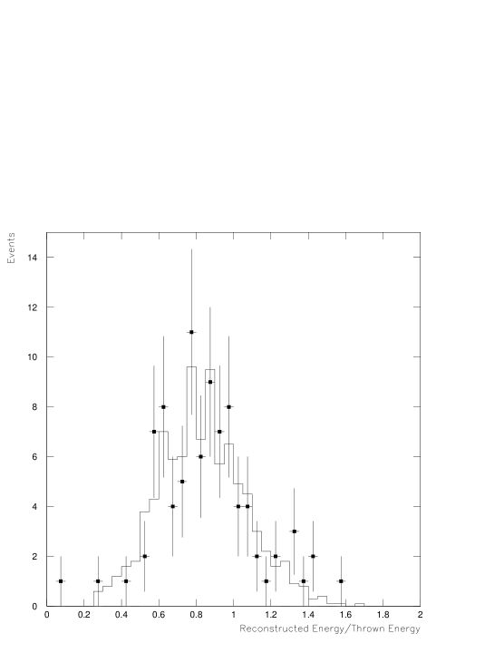
Figure 13: Ratio of HiRes-I reconstructed energy to thrown energy. The histogram is for Monte Carlo events. The black points show stereo events from the data where the Monte Carlo thrown energy has been replaced with the energy calculated from the stereo geometric reconstruction.

Figure 14: Scatter-plot of energy reconstructed by HiRes-I using the profile constrained geometry fit versus the energy reconstructed by HiRes-I using the stereo geometry for a set of stereo events.

Our Monte Carlo describes the HiRes-I data well. As an example, Figure 15 is a comparison between data and Monte Carlo of $R_{p}$, the impact parameter of showers, for events where $18.4<\log{E(eV)}<18.6$. The agreement is excellent.

Figure 15: Comparison between data and Monte Carlo for $R_{p}$, the impact parameter of showers, for events where $18.4<\log{E(eV)}<18.6$

7 Systematic Uncertainties

The largest sources of systematic uncertainty in this experiment are atmospheric modeling, the absolute calibration of the detector in units of photons, the absolute yield of the fluorescence process, and the correction for unobserved energy in the shower.

To test the sensitivity of the flux measurement at HiRes-II to uncertainties in atmospheric conditions we reanalyzed the data and generated new Monte Carlo samples with new conditions: we first changed the aerosol horizontal extinction length from 22 to 20 km, then we changed the aerosol scale height from 1.1 km to 0.7 km. The extinction length change corresponds to one standard deviation. For the scale height change we used the RMS of the scale height distribution, and thus made a conservative estimate of the systematic uncertainty from this source. These two variables are related since the aerosol column depth is equal to their product (for an exponential atmospheric model). Changing the horizontal extinction length had little effect, raising the normalization of $J(E)$ by $(4\pm 6)$%. The change in aerosol scale height had a larger effect, lowering $J(E)$ on average by $(15\pm 5)$%. We also raised the scale height and found a symmetric change in $J(E)$.

The systematic uncertainties in the HiRes-I data from atmospheric conditions are similar to those for HiRes-II. We found the reconstructed geometries of HiRes-I events above $10^{18.5}$ eV to be insensitive to changes in either the aerosol extinction length or the aerosol scale height, and we saw a maximum change in the energy of $\pm{13}$% at $10^{20}$ eV, decreasing to $\pm{6}$% at $10^{18.5}$ eV. Taking the average energy shift, 9%, the systematic uncertainty in flux from atmospheric effects at HiRes-I becomes $\pm{15}$%.

The systematic uncertainty from the absolute calibration of the detector is equal to 10% and is independent of energy[12]. The absolute uncertainty in the fluorescence yield is 10% and is independent of energy[16]. The uncertainty in the correction for unobserved energy in the shower is 5%[19]. Adding the uncertainties in quadrature yields a net systematic uncertainty on $J(E)$, averaged over energy, of 31%.

8 Discussion

In Figure 16, the monocular spectra from both the HiRes-I and HiRes-II detectors are shown[25]. In the energy range where both detectors’ data have good statistical power the results agree with each other very well. The highest energy HiRes-I data point corresponds to two events reconstructed at $1.0$ and $1.5\times 10^{20}$ eV.

We now fit the combined HiRes-I and HiRes-II monocular spectra to both a single power law fit and a double power law fit with a floating break point. The single power law fit results in a spectra index, $\gamma=-3.07\pm 0.02$, with a $\chi^{2}=67.8$ for 31 degrees of freedom. This is not an acceptable fit. The double power law fit results in a spectral index, $\gamma_{1}=-3.17\pm 0.03$ below the break point, $\log_{10}E=18.65\pm 0.05$, and a spectral index, $\gamma_{2}=2.89\pm 0.04$, above the break point. The $\chi^{2}$ for this fit was 41.1 for 29 degrees of freedom. The large improvement in the $\chi^{2}$ (26.7 while adding only two parameters) indicates strong evidence for the ankle being present in the combined HiRes monocular data.

The latest results of the AGASA experiment are also shown in this figure[5]. Below about $1\times 10^{20}$ eV the AGASA results are consistently a factor of two higher than ours. Above this energy their data points diverge from the trend of our data. Since the vertical axis in Figure 16 is $E^{3}\times J(E)$ a modest change in the energy scale would bring the experiments into considerably better agreement. For example lowering the AGASA energy scale by 30% would bring their points down by a factor of 2, move them to the left by 0.15 in $\log(E)$, and reduce the discrepancy between the two experiments. Such a change is within the systematic uncertainties of each experiment.

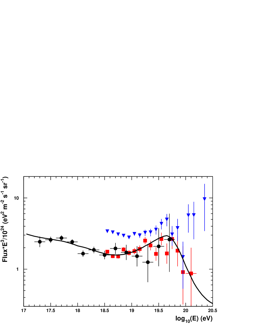
Figure 16: E³ times the UHE Cosmic Ray Flux. Results from the HiRes-I and HiRes-II detectors, and the AGASA experiment are shown. Also shown is a fit to the data assuming a model, described in the text, of galactic and extragalactic sources.

In the energy range, $18.7<\log{E}<19.8$ the HiRes data is fit by an $E^{-2.8}$ power law. The three highest-energy data points do not lie along an extension of that power law. Such an extension would predict that 25.3 events would occur above $\log{E}=19.8$ while only 10 were seen. The Poisson statistics probability of observing 10 or fewer events while expecting 25.3 is $4.9\times 10^{-4}$.

On the other hand, our data are consistent with the prediction of a GZK cutoff. As an example of what one would expect we have fit the data to a model that consists of two sources for cosmic rays, galactic and extragalactic, which includes the GZK threshold[26]. We use the extragalactic propagation model of Berezinsky, Gazizov, and Grigorieva[27], modified to take account of discrete energy losses of protons as in the paper by Blanton, Blasi and Olinto[28], and assume that protons come from sources distributed uniformly following the expansion of the universe, and lose energy by pion and $e^{+}e^{-}$ production from the cosmic microwave background radiation, as well as from the expansion of the universe. Since the measured composition[29, 30] changes from heavy to light within our energy range, we approximate the galactic component of cosmic rays as being the fraction of iron. We take this fraction to be 55% at $10^{17}$ eV, decreasing linearly with $\log{E}$ to 20% at $10^{17}$ eV, then decreasing to zero at $10^{20}$ eV. The model includes an end to the extragalactic input spectrum at $1\times 10^{21}$ eV. The fitting parameters of the model are the normalization and power law index (at the source) of extragalactic cosmic rays. The power law index in the fit was -2.4. The fit is excellent with $\chi^{2}$ of 32.6 for 31 degrees of freedom. In this model, the peak at $\log{E}$ of 19.8 is due to fitted $E^{-2.4}$ input spectrum being cut off at the pion production threshold, the ankle is due to energy losses from $e^{+}e^{-}$ production, and the second knee comes from the $e^{+}e^{-}$ production threshold.

9 Conclusions

We have measured the flux of UHE cosmic rays with the FADC detector of the HiRes experiment. Use of Flash ADC information allowed us to reduce systematic errors in reconstruction of events. We developed our Monte Carlo simulation programs to very accurately model the experiment, and calculated the exposure of the experiment in a way that takes into account the experimental resolution. The result reported here is in good agreement with the cosmic ray flux measurement made with the HiRes-I detector. The latter measurement is based on a largely statistically independent data set, with only a limited number of stereo events in common to both analyses. The result reported here is also consistent with the flux measured by the Fly’s Eye experiment using the stereo reconstruction technique. Above $10^{20}$eV our data is significantly different from that of the AGASA experiment. The ankle is not seen in the HiRes-II monocular alone, but is apparent in the combined HiRes-I and HiRes-II data. We have fit our data to a model incorporating both galactic and extragalactic sources of cosmic rays, which includes the GZK cutoff, and find good agreement.

10 Acknowledgements

This work is supported by US NSF grants PHY-9321949, PHY-9322298, PHY-0098826, PHY-0245428, PHY-0305516, PHY-0307098, by the DOE grant FG03-92ER40732, and by the Australian Research Council. We gratefully acknowledge the contributions from the technical staffs of our home institutions. The cooperation of Colonels E. Fischer and G. Harter, the US Army, and the Dugway Proving Ground staff is appreciated.

References

- [1] R.J. Protheroe, Topics in Cosmic Ray Astrophysics (ed. M.A. DuVernois, Nova Science Publishing, NY, 1999) and astro-ph/9812055.
- [2] K. Greisen, Phys. Rev. Lett. 16, 748 (1966); G. T. Zatsepin and V. A. Kuzmin, Pis’ma Zh. Eksp. Teor. Fiz. 4, 114 (1966) [JETP Lett. 4, 78 (1966)].
-
[3]
J. Linsley, Phys. Rev. Lett. 10, 146 (1963)
and Proc. 8th Int. Cosmic Ray Conf. 4, 295 (1963).
M.A. Lawrence, R.J.O. Reid, and A.A. Watson, J. Phys. G Nucl. Part. Phys. 17, 733 (1991) and references therein.
B.N. Afanasiev et al., Proc. Tokyo Workshop on Techniques for the Study of Extremely High Energy Cosmic Rays (ed. M. Nagano, Inst. for Cosmic Ray Research, Univ. of Tokyo), 35 (1993). - [4] D. J. Bird et al., Phys. Rev. Lett. 71, 3401 (1993) and Astrophys. J. 441, 144 (1995). See also T. Abu-Zayyad et al., Astrophys. J. 557, 686 (2001).
- [5] M Takeda et al., Astropart. Phys. 19, 447 (2003).
- [6] A.A. Watson, Proc. 25th Int. Cosmic Ray Conf. (Durban), 8, 257 (1997) and references therein.
- [7] M. Nagano et al., J. Phys. G. 10, 1295 (1984) and M. Nagano et al., J. Phys. G. 17, 733 (1991).
- [8] M. Ave et al., Proc. 27th Int. Cosmic Ray Conf. (Hamburg) 1, 381 (2001). See also astro-ph/0112253.
- [9] M.I. Pravdin et al., Proc. 26th Int. Cosmic Ray Conf. (Salt Lake City), 3, 292 (1999) and M.I. Pravdin et al., Proc. 28th Int. Cosmic Ray Conf. (Tuskuba), 389 (2003).
- [10] T. Abu-Zayyad et al., Proc. 26th Int. Cosmic Ray Conf. (Salt Lake City), 5, 349 (1999).
- [11] J. Boyer, B. Knapp, E. Mannel, and M. Seman, Nucl. Instr. Meth. A482, 457 (2002).
- [12] R.U. Abassi et al., to be submitted to Nucl. Instr. Meth.
- [13] R.U. Abassi et al., in preparation, and http://www.cosmic-ray.org/atmos/.
- [14] R. Baltrusaitis et al., Nucl. Inst. and Meth. A240, 410 (1985). See also P. Sokolsky, “Introduction to Ultrahigh Energy Cosmic Ray Physics,” (Cambridge University Press, 1990).
- [15] A. N. Bunner, Ph.D. Thesis, Cornell University, Ithaca, NY (1964).
- [16] F. Kakimoto et al., Nucl. Instr. Meth. A372, 527 (1996). See also G. Davidson and R. O’Neil, J. Chem. Phys. 41, 3946 (1964).
- [17] T. K. Gaisser and A. M. Hillas, Proc. 15th Int. Cosmic Ray Conf. (Plovdiv), 8 353, (1977).
- [18] T. Abu-Zayyad et al., Astropart. Phys. 16, 1 (2001).
- [19] C. Song et al., Astropart. Phys. 14, 7 (2000). See also J. Linsley, Proc. 18th ICRC, Bangalore, India, 12, 144 (1983) and R.M. Baltrusaitis et al., Proc. 19th ICRC, La Jolla, USA, 7, 159 (1985).
- [20] Heck, D., Knapp, J., Capdevielle, J. N., Schatz, G., Thouw, T., Report FZKA 6019 (1998), Forschungszentrum Karlsruhe; http://www-ik3.fzk.de/ heck/corsika/physics_description/ corsika_phys.html
- [21] N. N. Kalmykov, S. S. Ostapchenko, A. I. Pavlov, Nucl. Phys. B (Proc. Suppl.) 52B, 17 (1997).
- [22] G. Cowan, “Statistical Data Analysis,” Oxford Univ. Press, NY, (1998); see Chapter 11.
- [23] T. Abu-Zayyad et al., Astrophys. J. 557, 686 (2001).
- [24] R.U. Abassi et al., to be submitted to Astropart. Phys.
- [25] R.U. Abassi et al., accepted by Phys. Rev. Lett., astro-ph/0208243.
- [26] See R.U. Abassi et al., in preparation. See also E. Waxman, Astrophys. J. Lett. 452, L1 (1995); and J.N. Bahcall and E. Waxman, Phys. Lett. B556, 1 (2003).
- [27] V. Berezinsky, A.Z. Gazizov, S.I Grigorieva, hep-ph/0204357. See also S.T. Scully and F.W. Stecker, Astropart. Phys. 16, 271 (2002).
- [28] M. Blanton, P. Blasi and A.V. Olinto, Astropart. Phys. 15, 275 (2001).
- [29] T. Abu-Zayyad et al., Phys. Rev. Lett. 84, 4276, (2000).
- [30] R. Abbasi et al., submitted to Ap. J., astro-ph/0407622.