O and Ne K absorption edge structures and interstellar abundance
towards Cyg X-2

Abstract

We have studied the O and Ne absorption features in the X-ray spectrum of Cyg X-2 observed with the Chandra LETG. The O absorption edge is represented by the sum of three absorption-edge components within the limit of the energy resolution and the photon counting statistics. Two of them are due to the atomic O; their energies correspond to two distinct spin states of photo-ionized O atoms. The remaining edge component is considered to represent compound forms of oxide dust grains. Since Cyg X-2 is about 1.4 kpc above the galactic disk, the H column densities can be determined by radio (21 cm and CO emission line) and ${\rm H}_{\alpha}$ observations with relatively small uncertainties. Thus the O abundance relative to H can be determined from the absorption edges. We found that the dust scattering can affect the apparent depth of the edge of the compound forms. We determined the amplitude of the effect, which we consider is the largest possible correction factor. The ratio of column densities of O in atomic to compound forms and the O total abundance were respectively determined to be in the range $1.7^{+3.0}_{-0.9}$ to $2.8^{+5.1}_{-1.5}$ (ratio), and $0.63\pm 0.12$ solar to $0.74\pm 0.14$ solar (total), taking into account the uncertainties in the dust-scattering correction and in the ionized H column density. We also determined the Ne abundance from the absorption edge to be $0.75\pm 0.20$ solar. These abundance values are smaller than the widely-used solar values but consistent with the latest estimates of solar abundance.

1 Introduction

The metal abundance in the interstellar medium (ISM) is an important parameter for the understanding of the chemical evolution of the Universe. However, large uncertainties remain in our knowledge of this abundance. The solar abundance is sometimes regarded as the average of our Galaxy. However, UV absorption lines due to interstellar gas and optical absorption lines in the atmosphere of young B-stars have indicated that the metal abundance in the ISM of our Galaxy is on average about two thirds of the solar abundance (Savage & Sembach, 1996; Snow & Witt, 1996). However, both methods contain uncertainties because the former method is only sensitive to matter in atomic forms, while the abundance of B-star atmospheres may be different from the ISM. Indeed, Sofia & Meyer (2001) recently claimed that B-star abundances are lower than the ISM abundance and that the solar abundance is close to the ISM abundance. Moreover, the O solar abundance itself is not determined well. Recent values by Grevesse & Sauval (1998) and Holweger (2001) are significantly lower than the values in the widely used table of Anders & Grevesse (1989).

High resolution X-ray spectroscopy of absorption features due to the interstellar matter is a powerful tool to measure the amount of interstellar metal. It is sensitive to both the atomic (gas) and compound (molecular and dust grain) forms and can distinguish them by the chemical shifts. There are absorption lines and edges of many elements in the X-ray energy range. We can determine the column densities of these elements in different forms separately, integrating towards the X-ray source. However, the observation requires both high energy resolution and good statistics. Schatternburg & Canizares (1986) determined the O column density towards the Crab nebula with the transmission grating on the Einstein observatory. They could not separate atomic and compound forms. Also they were not able to determine the O abundance since the H column density towards the Crab nebula was not known. Paerels et al. (2001) analyzed the O and Ne absorption structures of the X-ray binary X0614+091 observed with the low energy transmission grating (LETG) on the Chandra observatory. They successfully separated the absorption features of O in atomic and compound forms. They also determined the abundance ratio of Ne to O. However, they could not determine the O abundance because the H column density toward the source is not known. Schulz et al. (2002) determined the column densities of O, Ne, Mg, Si, and Fe towards Cyg X-1 with the Chandra high energy transmission grating (HETG) data. They discussed the abundances of O, Ne, and Fe. However, it was necessary to assume the abundances of all other elements to be solar, in order to estimate the H column density towards Cyg X-1 from the X-ray spectrum.

In this paper we analyze the spectrum of Cyg X-2 obtained with the Chandra LETG and HRC (High Resolution Camera)-I. Cyg X-2 is a Low-Mass X-ray Binary (LMXB) located at ($l$,$b$)= ($87.33^{\circ}$,$-11.32^{\circ}$) and its distance is determined to be 7.2 kpc from the optical counterpart and X-ray burst with mass ejection (Cowley, Crampton, & Hutchings, 1979; Smale, 1998; Orosz & Kuulkers, 1999). Smale (1998) claimed a distance of 11.6 kpc, however, this is because he assumed the Eddington luminosity for a hydrogen rich atmosphere. If we assume a helium rich atmosphere, which is more realistic for type-I bursts (Lewin, van Paradijs, & Taam, 1995), the distance is consistent with 7.2 kpc. Adopting this distance, Cyg X-2 is located $\sim$ 1.4 kpc above the Galactic disk. Thus the H column density towards Cyg X-2 can be estimated from 21 cm (H I), CO (${\rm H}_{2}$), and ${\rm H}_{\alpha}$ (H II) observations with relatively small errors. Because of the featureless X-ray spectrum of the LMXB, the high brightness, and the well-determined H column density to the source, Cyg X-2 is one of the best X-ray sources for the study of the interstellar abundance with X-ray absorption.

In the next section, we will first discuss the H column density towards Cyg X-2. Then in the following sections we will show the observational results and discuss the O and Ne abundances and the uncertainties of the present results.

Throughout this paper, we quote single parameter errors at the 90 % confidence level unless otherwise specified.

2 H column density towards Cyg X-2

Interstellar hydrogen is distributed in three different forms; atomic (H I), molecular (H₂), and ionic (H II).

The column density of atomic hydrogen is measured by the 21 cm radio emission. In the H I map of Dickey & Lockman (1990), the H column density ($N_{\rm H}$) is given at grid points of 0.8 degree separation. By interpolating between the values of nearby points, the column density in the direction of Cyg X-2 is estimated to be $N_{\rm H}(\mathrm{atom})$=$2.17\times 10^{21}~{}\mathrm{cm^{-2}}$. Since the scale height of atomic hydrogen is $\sim 140$ pc, the total column density of our galaxy can be regarded as the column density to Cyg X-2. The standard deviation of the $N_{\rm H}$ values within two degrees of Cyg X-2 is $0.1\times 10^{21}~{}\mathrm{cm^{-2}}$. The power spectra of the small-scale spatial fluctuation of the galactic $N_{\rm H}(\mathrm{atom})$ were measured for different directions (Crovisier & Dickey, 1983; Dickey et al., 2001). On the spatial scales less than 1 deg, the power-law index of the power spectra is in the range from $-3$ to $-4$. Assuming the same shape of the power spectrum for the spatial fluctuations in the vicinity of Cyg X-2, we estimate the rms amplitude of the spatial fluctuation less than 2 degrees to be $0.12\times 10^{21}~{}\mathrm{cm}^{-2}$ and regard this as the 1-$\sigma$ error of the estimation.

Miramond & Naylor (1995) determined the upper limit of molecular hydrogen column density towards Cyg X-2 from the upper limit of CO emission line in the direction of Cyg X-2 to be $0.05\times 10^{21}~{}\mathrm{cm}^{-2}$ (90 % significance level). According to them, the contribution of H₂ in $N_{\rm H}$ is smaller than $0.10\times 10^{21}~{}\mathrm{cm}^{-2}$.

The total neutral H column density ($N_{\mathrm{HI}}+2N_{\mathrm{H_{2}}}$) is thus estimated to be $2.17^{+0.22}_{-0.20}\times 10^{21}~{}\mathrm{cm^{-2}}.$ On the other hand, the reddening towards Cyg X-2 is determined to be $E(B-V)\simeq 0.4$ (McClintock et al., 1984). Combining this with the relation, $N_{\mathrm{HI}}+2N_{\mathrm{H_{2}}}=5.8\times 10^{21}~{}E(B-V)~{}\mathrm{atoms~{}cm^{-2}~{}mag^{-1}}$ (Bohlin, Savage, & Drake, 1978), we obtain $N_{\mathrm{HI}}+2N_{\mathrm{H_{2}}}\simeq 2.3\times 10^{21}~{}\mathrm{cm^{-2}},$ which is consistent with the above estimation.

A large fraction ($\sim 97$ %, Mathis, 2000) of ionized H atoms exists in the warm ionized interstellar medium (WIM) of temperature $T\sim 8000$ K, distributed in our galaxy with a scale height $h$ of $\sim 900$ pc and a volume filling factor $f$ of $\gtrsim 0.2$. In the WIM, oxygen is effectively ionized through the charge exchange process. The number densities of neutral/ionized oxygen and hydrogen are related to $N$(O II)$/N$ (O I) = (8/9) $N$(H II)$/N$(H I) (Field & Steigman, 1971). According to more recent model calculations by Sembach et al. (2000), the ionization fraction of Ne is also similar to that of H; in their ‘COMPOSITE’ model, the values of $\log(N(X^{i})/N(X_{\rm total}))$ where $X=$ H, O, or Ne and $i$ represents the ionization states are, respectively, $-0.73$ and $-0.09$ for H I and H II, $-0.71$ and $-0.09$ for O I and O II, and $-0.70$ and $-0.10$ for Ne I and Ne II. Therefore, $N(X_{\rm total})/N({\rm H}_{\rm total})=N(X^{0})/N$(H I) is a good approximation for gas-phase O and Ne and we do not need to consider ionized H when we calculate atomic O and Ne abundances.

On the other hand, since interstellar dust grains are thought to co-exist with the WIM, we need to take into account the column density of ionized H when we estimate the abundance of O in compound forms. We estimated it from the H_α emission line intensity in the direction of Cyg X-2 obtained from the Wisconsin H-Alpha Mapper (WHAM) survey (Haffner et al., in prep, ) . The intensity is $14.6\pm 3.8$ Rayleighs. From the line intensity, the total emission measure in the column towards Cyg X-2 is estimated to be $(1.28\pm 0.33)\times 10^{20}(T/8000~{}\mathrm{K})~{}\mathrm{cm}^{-5}$, where we applied an extinction correction factor of 1.3 assuming $R_{\rm v}=3.1$ (Mathis, 1990). Assuming the spatial distribution described above, the emission measure and the column density are respectively related to the local ionized H density in the galactic plane, $n_{0}$, by,

$$EM=f\cdot n_{0}^{2}\int_{0}^{\infty}\left[\exp\left(-\frac{x\sin b}{h}\right)\right]^{2}dx$$

and

$$N_{\rm H}(\mathrm{ion})=f\cdot n_{0}\int_{0}^{d}\exp\left(-\frac{x\sin b}{h}\right)dx,$$

where $d$ and $b$ are the distance and the galactic latitude of Cyg X-2, respectively. From these we obtain $N_{\rm H}(\mathrm{ion})=0.70\pm 0.18\times 10^{21}(f/0.2)^{1/2}~{}\mathrm{cm}^{-2}$. As a nominal value, we adopted $N_{\rm H}(\mathrm{ion})=0.70\pm 0.18\times 10^{21}~{}\mathrm{cm}^{-2}$ ($f=0.2,$ Mathis, 2000) and thus $N_{\rm H}(\mathrm{total})=2.87^{+0.25}_{-0.23}\times 10^{21}~{}\mathrm{cm}^{-2}.$ Even for $f=1$, $N_{\rm H}(\mathrm{ion})$ does not exceed $1.57\pm 0.40\times 10^{21}~{}\mathrm{cm}^{-2}.$

In Table 1, we summarize the H column densities estimated in this section.

3 Analysis and results

3.1 Data reduction

Cyg X-2 was observed with the LETG/HRC-I for 30 ks on 2000 April 24 (obsID 87). We retrieved the archival data from the CXC (Chandra X-ray Center). Cyg X-2 is known to show both intensity and spectral variations. However, since the X-ray flux varied only $\sim 20~{}\%$ during the observation and since we are interested only in the interstellar absorption features, we integrated all the data after the standard data screening.

Since the spectrum in the archival data we retrieved is known to contain some processing errors, we reprocessed the data according to the standard methods described in threads in CIAO 2.2.1 (CALDB 2.10). We first obtained the spectra of the positive and negative orders. Then we summed them, rebinned to 0.025 Å  bins, and subtracted the background. The background was only $\sim 2~{}\%$ of the source counts in the wavelength region we used in the later analysis.

HRC-I has almost no energy resolution. The spectrum we obtained contains photons not only of the first order dispersion but also of the higher orders. We subtracted the higher order spectra utilizing the method described in Paerels et al. (2001). The $m$-th order spectrum of photons with a wavelength of $\lambda$ appears in the wavelength bin, $\hat{\lambda}=m\lambda$, of the first order spectrum. Since the LETG/HRC-I system has no detection efficiency below the wavelength $\lambda_{0}$, where $\lambda_{0}=1$ Å, we can neglect the contribution of the $m$-th order spectrum in the wavelength range $\hat{\lambda}<m\lambda_{0}$. From the spectrum in the range $\lambda_{0}<\hat{\lambda}<2\lambda_{0}$ and the efficiency ratio of the second to the first order spectra, we can estimate the second order spectrum in the range $2\lambda_{0}<\hat{\lambda}<4\lambda_{0}$ and subtract it from the total spectrum to obtain the first order spectrum in $\lambda_{0}<\hat{\lambda}<3\lambda_{0}$. In the same manner, we can subtract higher order spectra from all the wavelength range. We calculated the efficiency ratio from the effective areas of the LETG/HRC-S system provided at the CALDB WWW page because the higher order efficiencies are not available for the LETG/HRC-I system and because the efficiency ratios are not dependent on the detector. The calibration files we used are updated compared to those used by Paerels et al. (2001). We show in Figure 1 the spectra with and without higher orders.

We estimated the statistical errors of the first order spectrum obtained with the above method considering the error propagations. Because of the error propagations, the statistics of the spectral bins are no longer completely independent. However, the increase of the statistical errors after the higher order subtraction is smaller than 3% in the wavelength ranges we use in the following analysis. We thus treat them to be independent in the spectral fittings.

According to the LETGS calibration report at the CXC , the wavelength calibration of LETGS spectra is accurate to 0.02 %. This is smaller by an order of magnitude than the statistical errors in the wavelengths determined in the following analyses.

3.2 O absorption structure and the optical depth

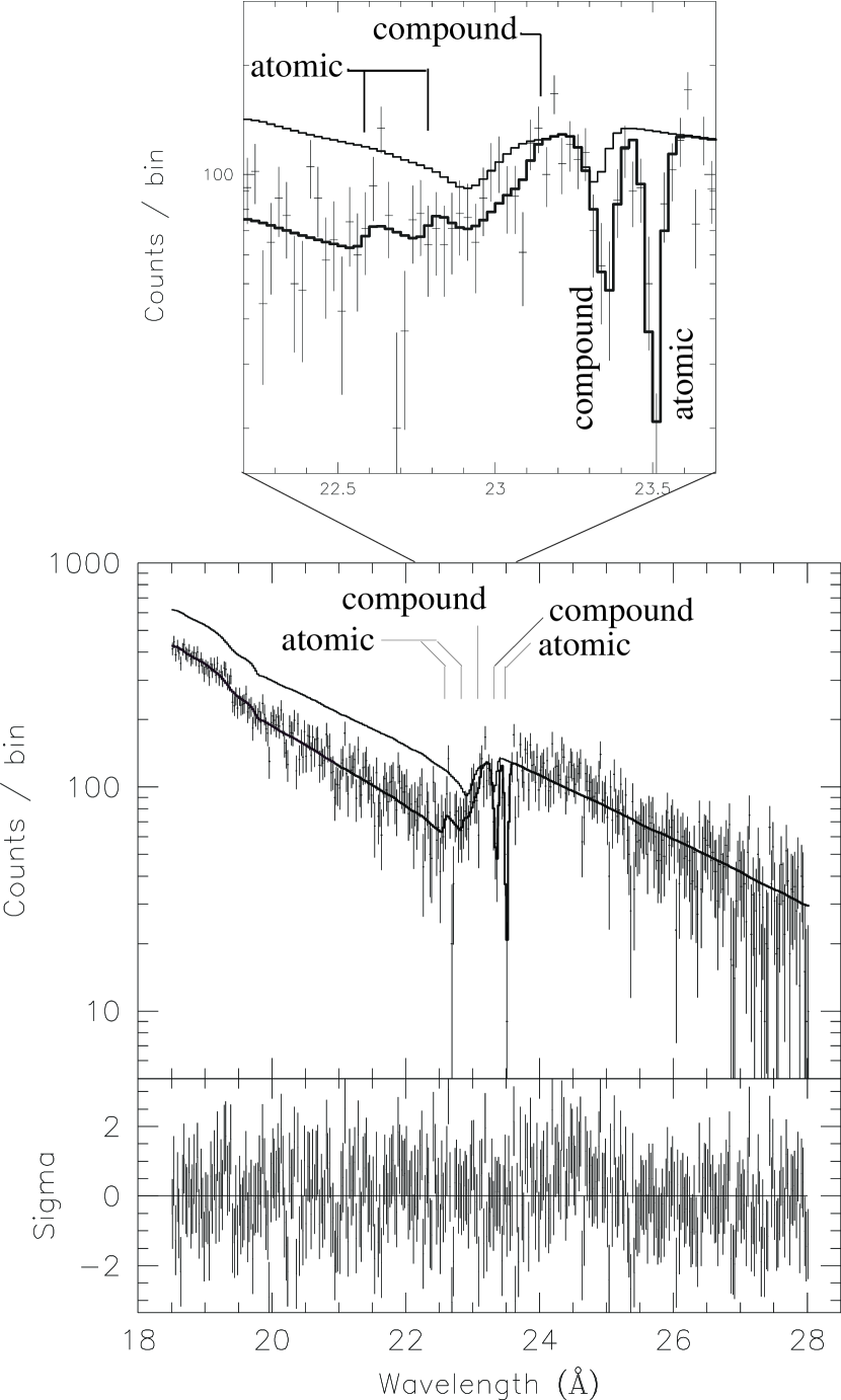
Figure 2: Spectral fit in the wavelength range including the O absorption structures. The whole wavelength range used in the spectral fits is shown in the lower graph, while in the upper graph the narrow wavelength range containing O edges and absorption lines is expanded. In the upper graph and in the upper panel of the lower graph, the observed 1st order spectrum is shown with data points with vertical bars which represent 1-$\sigma$ statistical errors. The best-fit model function of the three edge-component model (the last column of Table 2) convolved with the telescope and the detector response functions is shown with a thick line. The model function without O edges and absorption lines is shown with a thin line, in order to show the instrumental O absorption structure. Two absorption lines and an extended O edge clearly exist. In the lower panel of the lower graph, the residuals of the fit are shown

In the observed spectrum of Cyg X-2, we clearly found two absorption lines and an absorption edge near $\lambda\sim$ 23 Å besides the instrumental O absorption line and edge (see Figure 2). The centroid energies of the two absorption lines were determined to be $23.505\pm 0.007$ Å and $23.360\pm 0.014$ Å, and thus they were identified with the 1s–2p resonant lines of the atomic and compound O, respectively. However, since the absorption lines are saturated ($\tau\gg 1$), the absorption column densities cannot be determined accurately from the absorption lines. We thus focus on the absorption edge.

The absorption edge structure was extended compared to the instrumental O K-edge, which suggests that the edge structure consists of absorption edge components with different edge energies.

A complicated structure is expected for the absorption edge of an atomic O, firstly because photo-ionized O atoms take two distinct final states with different total spin numbers, and secondly because there are many absorption lines which cannot be resolved with the LETGS near the absorption edges (McLaughlin & Kirby, 1998). The theoretical values of edge energies calibrated with ground experiments are 544.03 eV (22.790 Å, spin 3/2) and 548.85 eV (22.590 Å, spin 1/2) (McLaughlin & Kirby, 1998). On the other hand, the edge energy of the compound O depends on the chemical state. Thus the absorption edge of the compound forms can have an extended structure. The edge energy must be lower than the edge energy of atomic O, but higher than the absorption line energy. According to Sevier (1979), the edge energy of O in metal oxide is $532.0\pm 0.4$ eV ($23.31\pm 0.02$ Å).

All the O edge structures may not be identified because the statistics and the energy resolution of the present data are limited. Thus, we first apply a rather simple model to the observed spectrum, then later try more and more complicated models.

We restricted the wavelength range of model fits in order to avoid the contributions of absorption edges of other elements. We did all the analysis described below with several different wavelength ranges. We found that the O absorption optical depth determined from the analysis is not dependent on the wavelength ranges of the fits, so long as the lower and upper limits of the range are within the ranges 17.5–19.0 Å and 27.0–29.0 Å, respectively. Thus we show here the results with the fitting range of 18.5 Å–28.0 Å.

We assumed a power-law function for the continuum spectrum. We also included the absorption by neutral matter represented by the tbabs model in the ‘sherpa’ program (Wilms, Allen, & McCray, 2000) with the O abundance fixed to 0. We included an O absorption edge with a separate absorption edge component represented by edge model in the sherpa program. We fixed the H column density of the tbabs absorption model to $2.17\times 10^{21}~{}\mathrm{cm^{-2}}$ and fixed the helium abundance to the solar value. We performed the fits with the abundances of other atoms fixed at several different values between 0.5 and 1.5 solar. We found that the dependence of the best-fit O absorption optical depths on the abundance of other elements is only about ten percent of the statistical errors. Thus we only show the results with the abundance of other elements fixed at the solar values.

In the first model, we included two oxygen edge components. We treated the edge energies and the optical depths of the two ‘edge’ components as free parameters. We represented the two O absorption lines with negative Gaussian functions. We fixed the centroid wavelengths to 23.505 Å  and 23.360 Å, and the widths to 0.04 Å. The free parameters of the fits were the two O edge energies and optical depths, the normalization factor and the power-law index of the continuum, and the normalization factors of the two Gaussian absorption lines.

We show the results of the fits in the first data column of Table 2. The best fit energies of the two edges were $22.76^{+0.13}_{-0.04}$ Å and $23.11^{+0.09}_{-0.03}$ Å, respectively. The former is consistent with the atomic O edge of the spin 3/2 final state within the statistical error. On the other hand, the latter is in the middle of the atomic and the instrumental O absorption edges. Thus, it is likely to represent an O edge of compound forms.

Next, in order to investigate possible complex structures of the edges and the model dependence of the absorption optical depths, we increased the number of edge components one by one. In the fits, we allowed both the energies and optical depths of all the edges to vary. In the second and third data columns of Table 2, the results are summarized. The $\chi^{2}$ value shows a significant improvement from the double to the three edge models (99.6 % confidence with an F-test). The edge energy of the third edge is 22.58 Å= 549.1 eV. This energy is close to the edge energy for a final spin 1/2. In the raw spectrum (Figure 2), we can find this edge structure. On the other hand, the $\chi^{2}$ value did not improve from the three-edge to the four-edge models. Thus we conclude that the observed O edge structure can be represented with the three-edge model within the limit of the present statistics and the energy resolution; two of the edges represent absorption by atomic O corresponding to the two different O-ion spin states, and the remaining one represents absorption by O in compound forms.

Finally, in order to determine the spectral parameters and their statistical errors for the three-edge model more precisely, we performed the spectral fit with the three-edge model with the two edge energies of the atomic O fixed at the theoretical values. In the last column of Table 2, we show the results. We estimated the statistical error for the total optical depth for the atomic O edge from the $\chi^{2}$ contour map to find the total optical depth of $0.43\pm 0.14$. The optical depth of compound forms is $0.26\pm 0.11$.

To estimate the column density of O from the absorption optical depth, we adopted the absorption cross section of Verner & Yakovlev (1995): $\sigma_{\mathrm{abs}}=4.98\times 10^{-19}~{}\mathrm{cm^{2}}$ both for atomic and compound forms. We obtained $N_{\rm O,atom}=8.6\pm 2.8\times 10^{17}~{}\mathrm{cm^{-2}}$ and $N_{\rm O,comp}=5.2\pm 2.2\times 10^{17}~{}\mathrm{cm^{-2}}$.

Assuming the $N_{\rm H}$ values of $2.17^{+0.22}_{-0.20}\times 10^{21}~{}\mathrm{cm^{-2}}$ for atomic O and $2.87^{+0.25}_{-0.23}\times 10^{21}~{}\mathrm{cm^{-2}}$ for compound forms, we estimate the abundance of O to be $0.47\pm 0.16$ solar (atomic), $0.21\pm 0.09$ solar (compound), and $0.68\pm 0.13$ solar (total), where we assumed the O solar abundance of $8.51\times 10^{-4}$ (Anders & Grevesse, 1989). The error of the total abundance was estimated from the $\chi^{2}$ contour map of the spectral fit, taking into account the difference of $N_{\rm H}$ values for gas and compound forms and their systematic errors.

3.3 Absorption structure of Ne

In the observed spectrum of Cyg X-2, we also clearly found an absorption edge at 14.3 Å, which is identified with the Ne K-edge (Figure 3). We performed spectral fits to the wavelength range of 12.0–15.5 Å. In addition to the edge, there is an absorption line at 14.6 Å. Because the line wavelength is close to the edge, we included an absorption line in the model function. We employed the model function similar to that used for the O features. We represented the Ne edge with a single edge model.

In Table 3, we show the results of the fit. The absorption edge wavelength was consistent with that of the neutral Ne (14.25 Å; Verner & Yakovlev, 1995). From the optical depth determined from the fit and the theoretical absorption cross section of Ne I (Verner & Yakovlev, 1995), we determined the column density and abundance of Ne to be $2.00\pm 0.51\times 10^{17}~{}\mathrm{cm^{-2}}$ and $0.75\pm 0.20$ times the solar abundance of Anders & Grevesse (1989).

Although the absorption-line energy, $14.599\pm 0.012$ Å, is close to the resonant line energy of Ne II (14.631 Å, Behar & Netzer, 2002), it is outside the 90% statistical error domain. Thus we can not unequivocally identify this absorption line. However, if we assume it is Ne II, the column density estimated from the line is $8.0\pm 2.4\times 10^{16}~{}\mathrm{cm^{-2}}$, which is about 1/3 of Ne I. Thus if the absorption line is due to Ne II, Ne II can be attributed to the WIM.

4 Discussion

We have analyzed the O and Ne absorption structures in the X-ray spectrum of Cyg X-2 observed with the Chandra LETG/HRC-I. The O edge is represented by the sum of three edge components within the limit of present statistics and energy resolution. Two edge components represent absorptions by atomic O; their edge energies are consistent with the theoretical values corresponding to the two distinct final O states of different spin numbers. The edge energy of the remaining edge is lower than the other two, and is likely to represent O in compound forms. From the depth of the edges, we estimated the O column densities with atomic and compound forms separately.

We tried a four-edge component model in the spectral fits. We find the sum of the optical depths of all the edge components does not change significantly from three to four edge models. Thus we conclude that the total O column density does not depend significantly on the number of edge components assumed in the spectral models. We estimated the atomic, compound, and total O abundances to be $0.47\pm 0.16$, $0.21\pm 0.09$, and $0.68\pm 0.13$ times the solar abundance of Anders & Grevesse (1989) respectively. The Ne edge is represented with a single edge model and the Ne abundance is estimated to be $0.75\pm 0.20$ solar. In the errors of abundance quoted above, we included the statistical errors of the spectral fits, and the systematic errors of $N_{\rm H}$ estimated from the spatial fluctuation of 21cm and ${\rm H}_{\alpha}$ emissions and the upper limit of CO emission.

There is an additional systematic error in the abundance of O in compound forms, arising from the uncertainty in the spatial distribution of the WIM. If we consider the extreme case in which its volume filling factor is 1, the O abundance reduces to $0.16\pm 0.07$ (compound form) and $0.63\pm 0.12$ (total).

It is very unlikely that the O and Ne absorption edges are associated with the circumstellar matter in the Cygnus X-2 binary system. Suppose that the absorption column of $N_{\rm H}\sim 2\times 10^{21}{\rm cm}^{-2}$ is located in a distance $r$ from the X-ray source. The ionization parameter, $\xi=L_{\rm X}/(nr^{2})\sim L_{\rm X}/(N_{\rm H}r)$ must be smaller than $\sim 10$ so that O is neutral (Kallman & McCray, 1982). With $L_{\rm X}=10^{38}$ erg sec^-1, we find $r\gtrsim 10^{16}$ cm. This is much larger than the size of the binary system ($\sim 10^{12}$ cm, Cowley, Crampton, & Hutchings, 1979) This is consistent with the facts that all emission and absorption line features found in LMXBs are from highly ionized atoms (e.g., Asai et al., 2000; Cottam et al., 2001) and that low-ionization emission lines from the Cyg X-2 system are from near the companion star (Cowley, Crampton, & Hutchings, 1979).

About one third of O contributing to the absorption edges is in compound form. Dust grains are considered to contribute to this component. In such a situation, the optical depth for dust scattering of X-rays is not negligible compared to the absorption if we assume a typical dust radius of $\sim 0.1~{}\mu$m. Scattered X-rays form an extended halo on the few arcminute scale (Hayakawa, 1970; Mauche & Gorenstein, 1986; Predehl & Schmitt, 1995). Since the scattering cross section is dependent on the X-ray energy, the energy spectrum of the unscattered X-rays is modified by scattering. However, if multiple scattering is negligible and if the spatial distribution of dust is uniform over the spatial scale corresponding to the dust halo, the energy spectrum of total photons, i.e., the sum of the unscattered core and the scattered halo, is not modified by dust scattering. This is not the case for the present energy spectrum obtained with the LETG, since we derived the energy spectrum only from the central $\sim$ 1 arc second of the X-ray image. Because the scattering cross sections show anomalous features around absorption edges (Mitsuda et al., 1990), the dust scattering will affect the estimation of the absorption column density; the scattering cross section is smaller at the energy just above the edge (at the wavelength shorter than the edge), while the absorption cross section is larger. This leads to an underestimation of the O absorption column density. We estimated the amplitude of this effect in the following way.

The total scattering cross section of an X-ray photon of a wavelength $\lambda$ with a dust grain of a radius $a$ is given by

$$\sigma_{\mathrm{dust,sc}}=2\pi a^{2}\left(\frac{2\pi a}{\lambda}\right)^{2}\left|\frac{Nr_{0}\lambda^{2}}{2\pi}(f_{1}+{\rm i}f_{2})\right|^{2},$$

under the Rayleigh-Gans approximation (van de Hulst, 1957), where $N$ is the number of atoms per unit volume, $r_{0}$ is the classical electron radius, and $f_{1}$ and $f_{2}$ are the atomic scattering factors (Henke, Gullikson, & Davis, 1993). The Rayleigh-Gans approximation is valid for $(2\pi a/\lambda)|Nr_{0}\lambda^{2}/(2\pi)(f_{1}+{\rm i}f_{2})|\ll 1$.

Because the factor $|f_{1}+{\rm i}f_{2}|$ becomes small near the absorption edge, the dust scattering cross section is reduced at the edge. Assuming typical chemical compositions and densities of dust grains ($\mathrm{FeSiO_{4}}$, $\mathrm{FeSiO_{3}}$, $\mathrm{Mg_{2}SiO_{4}}$ and $\mathrm{MgSiO_{3}}$), we estimate the reduction of the scattering cross section at the O edge to be in the range,

$$\Delta\sigma_{\mathrm{dust,sc}}=(0.53-0.93)\times 10^{-10}\left(\frac{a}{0.1~{}\mathrm{\mu m}}\right)^{4}~{}\mathrm{cm}^{2}.$$

Assuming the number density of dust to be proportional to $\propto a^{-3.5}$ with a cut off at $a_{\mathrm{max}}$ (Mathis, Rumpl, & Nordsieck, 1977), we calculate the reduction of the scattering cross section per O atom,

$$\Delta\sigma_{\mathrm{sc}}=(0.74-1.44)\times 10^{-19}\left(\frac{a_{\mathrm{max}}}{0.1~{}\mathrm{\mu m}}\right)~{}\mathrm{cm}^{2}.$$

Thus the reduction of scattering cross section can be a few tens of percent of the absorption cross section, $\sigma_{\mathrm{abs}}=4.98\times 10^{-19}~{}\mathrm{cm^{2}}$. The maximum grain radius contributing to X-ray scatterings has been estimated from the spatial size of dust scattering halos. Mauche & Gorenstein (1986) and Mitsuda et al. (1990) suggested $a_{\mathrm{max}}=0.05-0.1~{}\mathrm{\mu m}$, but recently Witt, Smith, & Dwek (2001) suggested the presence of grains with radii as large as $0.5\mathrm{\mu m}$. Adopting $a_{\mathrm{max}}=0.1~{}\mathrm{\mu m}$, and assuming that O of compound forms are all in dust grains, the column density of O of compound forms increases from $5.2\times 10^{17}~{}\mathrm{cm^{-2}}$ to $(6.1-7.3)\times 10^{17}~{}\mathrm{cm^{-2}}$. At the O edge energy, the Rayleigh-Gans approximation is valid only for $a_{\mathrm{max}}~{}\lesssim 0.1~{}\mathrm{\mu m}$ and the scattering cross section saturates at $a_{\mathrm{max}}\gtrsim 0.1~{}\mathrm{\mu m}$ (Alcock & Hatchett, 1978; Smith & Dwek, 1998). Thus the correction factor does not increase for larger grains and the correction factor we applied above can be regarded as the maximum correction.

The O abundance values calculated for four different cases (with and without correction for dust scattering, and two different values of the volume filling factor of the WIM) are summarized in Table 4. The total O abundance is between $0.63\pm 0.12$ and $0.74\pm 0.14$ times solar. On the other hand the Ne abundance is $0.75\pm 0.20$. Our results are more consistent with the recent solar abundances than the most widely used ‘old’ values. For example , the O and Ne solar abundances by Holweger (2001) are 0.65 and 0.81 times the values in Anders & Grevesse (1989), respectively.

Another important parameter we can estimate from the present X-ray observation is the gas to dust ratio of the O column densities, which is estimated to be $2.2^{+3.9}_{-1.1}$, $2.8^{+5.1}_{-1.5}$, $1.7^{+3.0}_{-0.9}$, and $2.2^{+4.0}_{-1.1}$ for cases 1 to 4 of Table 4, respectively. This should be compared with the value estimated from the gas abundance from interstellar UV absorption lines and the assumption that the total abundance is solar. Adopting the O gas abundance of Cartledge, Meyer, & Lauroesch (2001) and solar abundances by Anders & Grevesse (1989) and Holweger (2001), we obtain 0.7 and 1.7, respectively. Our result is again consistent with the latest solar abundance value.

For O, the present X-ray result contains an additional uncertainty due to the correction for dust scattering. We can avoid this if we include the spectrum from the scattering halo in the analysis. This requires non-dispersive high resolution spectrometers such as microcalorimeters, which will be used on board future X-ray missions, such as Astro-E2.

Figure 1: The Cyg X-2 spectrum obtained with the Chandra LETG/HRC-I. The raw LETG spectrum containing higher order photons is shown with a thin line, while the spectrum after higher-order subtraction (see text) is shown with a thick line.

Figure 3: Spectral fit in the wavelength range including the Ne absorption structures. The observed 1st order spectrum with 1-$\sigma$ error bars and the best fit model function convolved with telescope and detector response functions are shown in the upper panel, and the residuals of the fit are shown in the lower panel.

Table 1: Hydrogen column density to Cyg X-2

Form of H		H column density
H I		$2.17\pm 0.20\times 10^{21}~{}\mathrm{cm^{-2}}$
${\rm H}_{2}$		$<0.10\times 10^{21}~{}\mathrm{cm}^{-2}$
H II	(nominal)(3)	$0.70\pm 0.18\times 10^{21}~{}\mathrm{cm^{-2}}$
H II	(maximum)(4)	$1.57\pm 0.40\times 10^{21}~{}\mathrm{cm^{-2}}$
H I+${\rm H}_{2}$ (1)		$2.17^{+0.22}_{-0.20}\times 10^{21}~{}\mathrm{cm^{-2}}$
All forms (2)	(nominal)(3)	$2.87^{+0.25}_{-0.23}\times 10^{21}~{}\mathrm{cm^{-2}}$
All forms (2)	(maximum)(4)	$3.74\pm 0.45\times 10^{21}~{}\mathrm{cm^{-2}}$

Table 2: Results of spectral fits of O K-edge absorption features

Parameters		Two Edges	Three Edges	Four Edges(1)	Three with two fixed(2)
Power-law
normalization	(photons s-1 keV-1 cm-2@555.2 eV)	$2.52\pm 0.07$	$2.53\pm 0.07$	2.53	$2.53\pm 0.07$
photon index		$0.74\pm 0.17$	$0.69^{+0.18}_{-0.16}$	0.70	$0.71\pm 0.17$
Absorption line 1
Centroid	(eV)	527.48	527.48	527.48	527.48
	(Å)	(23.51)	(23.51)	(23.51)	(23.51)
Equivalent width	(eV)	$1.41\pm 0.24$	$1.41\pm 0.24$	1.41	$1.41\pm 0.24$
Absorption line 2
Centroid	(eV)	530.76	530.76	530.76	530.76
	(Å)	(23.36)	(23.36)	(23.36)	(23.36)
Equivalent width	(eV)	$0.97\pm 0.28$	$0.97\pm 0.28$	1.0	$0.97\pm 0.28$
Absorption Edge 1
Edge energy	(eV)	$536.4^{+0.8}_{-1.9}$	536.2(3)	536.2	$536.1\pm 1.5$
	(Å)	($23.11^{+0.09}_{-0.03})$	(23.12)	(23.13)	($23.13\pm 0.06$)
Optical depth		$0.27\pm 0.10$	$0.24\pm 0.12$	0.24	$0.26\pm 0.11$
Absorption Edge 2
Edge energy	(eV)	$544.8^{+0.8}_{-3.1}$	542.3(3)	542.3	544.03
	(Å)	($22.76^{+0.13}_{-0.04}$)	(22.86)	(22.86)	(22.79)
Optical depth		$0.41^{+0.10}_{-0.08}$	$0.24^{+0.29}_{-0.13}$	0.19	$0.23^{+0.16}_{-0.11}$
Absorption Edge 3
Edge energy	(eV)		549.1(3)	544.9	548.85
	(Å)		(22.58)	(22.75)	(22.59)
Optical depth			$0.22^{+0.13}_{-0.15}$	0.09	$0.20^{+0.15}_{-0.17}$
Absorption Edge 4
Edge energy	(eV)			549.2
	(Å)			(22.58)
Optical depth				0.18
$\chi^{2}$/dof		400.45/371	397.40/369	397.163/367	398.21/371

Table 3: Results of spectral fits of Ne K-Edge

Parameters		Best fit value
Power-law
normalization	(photons s-1 keV-1 cm-2@1keV)	$1.685\pm 0.023$
photon index		$1.328^{+0.070}_{-0.072}$
Absorption line
Centroid	(eV)	$849.24\pm 0.68$
	(Å)	($14.559\pm 0.012$)
Equivalent width	(eV)	$0.541\pm 0.160$
Absorption Edge
Edge energy	(eV)	$866\pm 5$
	(Å)	($14.31^{+0.08}_{-0.09}$)
Optical depth		$0.059\pm 0.015$
$\chi^{2}$/dof		149.724/133

Table 4: Summary of interstellar O and Ne abundances

Atom	Form	Case 1a	Case 2b	Case 3c	Case 4d
O	gas phase	$0.47\pm 0.16$	$\rightarrow$	$\rightarrow$	$\rightarrow$
	compound	$0.21\pm 0.09$	$0.16\pm 0.07$	$0.27\pm 0.12$	$0.21\pm 0.09$
	total	$0.66\pm 0.12$	$0.63\pm 0.12$	$0.74\pm 0.14$	$0.68\pm 0.14$
Ne		$0.75\pm 0.20$

Note. — All abundance values are in units of the solar values of Anders & Grevesse (1989).

References

- Anders & Grevesse (1989) Anders, E., & Grevesse, N. 1989, Geochim. Cosmochim. Acta., 53, 197
- Asai et al. (2000) Asai, K., Dotani, T., Nagase, F., & Mitsuda, K. 2000, ApJS, 131, 571
- Alcock & Hatchett (1978) Alcock, C., & Hatchett, S. 1978, ApJ, 222, 456
- Behar & Netzer (2002) Behar, E, & Netzer, H. 2002, ApJ, 570, 165
- Bohlin, Savage, & Drake (1978) Bohlin, R. C., Savage, B. D., & Drake, J. F. 1978, ApJ, 224, 132
- Cartledge, Meyer, & Lauroesch (2001) Cartledge, S. I. B., Meyer, D. M., & Lauroesch, J. T. 2001, ApJ, 562, 394
- Cottam et al. (2001) Cottam, J., Kahn, S. M., Brinkman, A. C., den Herder, J. W., & Erd, C. 2001, A&A, 365, L277
- Cowley, Crampton, & Hutchings (1979) Cowley, A. P., Crampton, D., & Hutchings, J. B. 1979, ApJ, 231, 539
- Crovisier & Dickey (1983) Crovisier, J., & Dickey, J. M. 1983, A&A, 122, 282
- Dickey & Lockman (1990) Dickey, J. M., & Lockman, F. J. 1990, ARA&A, 28, 215
- Dickey et al. (2001) Dickey, J. M., McClure-Griffiths, N. M., Stanimirović, S., Gaensler, B. M., & Green, A. J. 2001, ApJ, 561, 264
- Field & Steigman (1971) Field, G. B., & Steigman, G. 1971, ApJ, 166, 59
- Grevesse & Sauval (1998) Grevesse, N., & Sauval, A. J. 1998, Space Sci. Rec., 85, 161
- (14) Haffner, L. M., Reynolds, R. J., Tufte, S. L., et al., in preparation
- Hayakawa (1970) Hayakawa, S. 1970, Progr. Theor. Phys., 43, 1224
- Henke, Gullikson, & Davis (1993) Henke, B. L., Gullikson, E. M., & Davis, J. C. 1993, Atom. Data and Nuc. Data Tab., 54, No. 2
- Holweger (2001) Holweger, H. 2001, in Solar and Galactic Composition, ed. R. F. Wimmer-Schweingruber (Berlin: Springer)
- Kallman & McCray (1982) Kallman, R., & McCray, R. 1982, ApJS, 50, 263
- Lewin, van Paradijs, & Taam (1995) Lewin, W. H. G. van Paradijs, J, Taam, R. E. 1995, in Cambridge Astrophysics Series 26, X-ray Binaries, ed. W. H. G. Lewin, J. van Paradijs, & E. P. J. van den Heuvel (Cambridge: Cambridge University Press), 175
- Mathis, Rumpl, & Nordsieck (1977) Mathis, J. S., Rumpl, W., & Nordsieck, K. H. 1977 , ApJ, 217, 425
- Mathis (1990) Mathis, J. S. 1990, ARA&A, 28, 37
- Mathis (2000) Mathis, J. S. 2000, in Allens’ Astrophysical Quantities, forth edition, ed. N. Cox (AIP and Springer-Verlag), 523
- Mauche & Gorenstein (1986) Mauche, C. W., & Gorenstein, P. 1986, ApJ, 302, 371
- McClintock et al. (1984) McClintock, J. E., Petro, L. D., Hammerschlag-Hensberge, G., Proffitt, C. R., & Remillard, R. A. 1984, ApJ, 283, 794
- McLaughlin & Kirby (1998) McLaughlin, B. M., & Kirby, K. P. 1998, J. Phys. B: At. Mol. Opt. Phys., 31, 4991
- Miramond & Naylor (1995) Miramond, L. K., & Naylor, T. 1995, A&A, 296, 390
- Mitsuda et al. (1990) Mitsuda, K., et al. 1990, ApJ, 353, 480
- Orosz & Kuulkers (1999) Orosz, J. A., & Kuulkers, E. 1999, ApJ, 305, 132
- Paerels et al. (2001) Paerels, F., et al. 2001, ApJ, 546, 338
- Predehl & Schmitt (1995) Predehl, P., & Schmitt, J. H. M. M., 1995, A&A, 293, 889
- Savage & Sembach (1996) Savage, B. D., & Sembach, K. R. 1996, ARA&A, 34, 279
- Schatternburg & Canizares (1986) Schatternburg, M. L., & Canizares, C. R. 1986, ApJ, 301, 759
- Schulz et al. (2002) Schulz, N. S., Cui, W., Canizares, C. R., Marshall, H. L., Miller, J. M. & Lewin, W. H. G. 2002, ApJ, 565, 1141
- Sembach et al. (2000) Sembach, K. R., Howk, C., Ryans, R. S. I., & Keenan, F. P. 2000, ApJ, 528, 310
- Sevier (1979) Sevier, K. D., 1979, Atom. Data and Nuc. Data Tab., 24, 323
- Smale (1998) Smale, A. P. 1998, ApJ, 498, L141
- Smith & Dwek (1998) Smith, R. K., & Dwek, E. 1998, ApJ, 503, 831
- Snow & Witt (1996) Snow, T. P., & Witt, A. N. 1996, ApJ, 468, L65
- Sofia & Meyer (2001) Sofia, U. J., & Meyer, D. M. 2001, ApJ, 554, L221
- van de Hulst (1957) van de Hulst 1957, Light Scattering by Small Particles (New York: Dover)
- Verner & Yakovlev (1995) Verner, D. A., & Yakovlev, D. G. 1995, A&AS, 109, 125
- Wilms, Allen, & McCray (2000) Wilms, J., Allen, A., & McCray, R. 2000, ApJ, 542, 914
- Witt, Smith, & Dwek (2001) Witt, A. N., Smith, R. K., & Dwek, E. 2001, ApJ, 550, L201