Structure of pulsar beams: conal versus patchy

Structure of mean pulsar radiation patterns is discussed within the nested-cones and patchy beam models. Observational predictions of both these models are analyzed and compared with available data on pulsar waveforms. It is argued that observational properties of pulsar waveforms are highly consistent with the nested-cone model and, in general, inconsistent with the patchy beam model.

1 Introduction

One of the important questions in pulsar research is what the overall structure of the mean pulsar beam is and how this structure is related to highly fluctuating instantaneous pulsar radiation. It is difficult to reveal this structure as pulsar observations represent one-dimensional cuts through two-dimensional beams. However, some indirect methods have been applied in an attempt to resolve this problem and two major models of pulsar beams have emerged from this work. Rankin (1993), Gil et al. (1993) and Kramer et al. (1994) calculated the opening angles $\rho$ of emission corresponding to a pulse width $W$ measured at 10 and 50 percent of the maximum intensity. As a result, they obtained a binomial distribution of these angles, that is, for a given period $P$ one of the two preferred values was possible, following however a general $P^{-1/2}$ dependence. Such distribution is most naturally interpreted as an indication of two nested cones in the structure of mean pulsar beams. This interpretation is called a conal model of pulsar beams. An alternative model postulates that the mean pulsar beam is patchy (Lyne & Manchester, 1988, LM88 hreafter), with different components randomly distributed within an almost circular “window function” (Manchester, 1995; Han & Manchester, 2001). Such a model is apparently inconsistent with the binomial distribution of the opening angles inferred from measured pulse widths. In fact, unless putative patches are distributed along nested-circular patterns, the distribution of corresponding opening angles should be (for any given period) random rather than binomial.

Recently, Mitra & Deshpande (1999, MD99 hereafter) attempted to test both these rival models. They distributed locations of the profile components (measured as the peak-to-peak separation of the outer conal components in complex profile pulsars) on one quadrant of the beam represented on the common normalised scale (with $x$-axis and $y$-axis representing longitudes $\varphi$ and impact angles $\beta$, respectively; refer to Fig. 4 of MD99). They found that most of the peak intensity points are concentrated in narrow sections of the beam. This feature is a strong indication of the conal structure of the pulsar beam. It can be argued that if, indeed, the pulsar beams are patchy, then in such a case there is a high probability for the beam to be uniformly filled with peak intensity locations. Further in their analysis, they excluded the so-called conal single and conal double profiles (Rankin, 1983), which are thought to be exclusively grazing cuts of the line-of-sight at the beam boundary. They found that such exclusion in their sample led to the absence of points at high impact angles $\beta$, which is perfectly consistent with the nested cone model and inconsistent with the patchy beam model. In fact, within the patchy beam model there is no reason why the single and double profiles occur exclusively at high impact angles. Moreover, the midpoint of single and double profiles usually coincides with the fiducial phase, at which the multifrequency profiles align after being corrected for cold plasma dispersive delays. This property is natural within the conal model and inconsistent (in general) with the patchy beam model, since patches would have to be placed symmetrically with respect to the fiducial plane, containing both magnetic ${\bf m}$ and spin ${\bf\Omega}$ axes (Fig. 1). As argued by MD and independently by Gil & Sendyk (2000, GS00 hereafter) the “mean” average pulsar beam consists of up to three nested cones, centered on the global magnetic dipole axis.

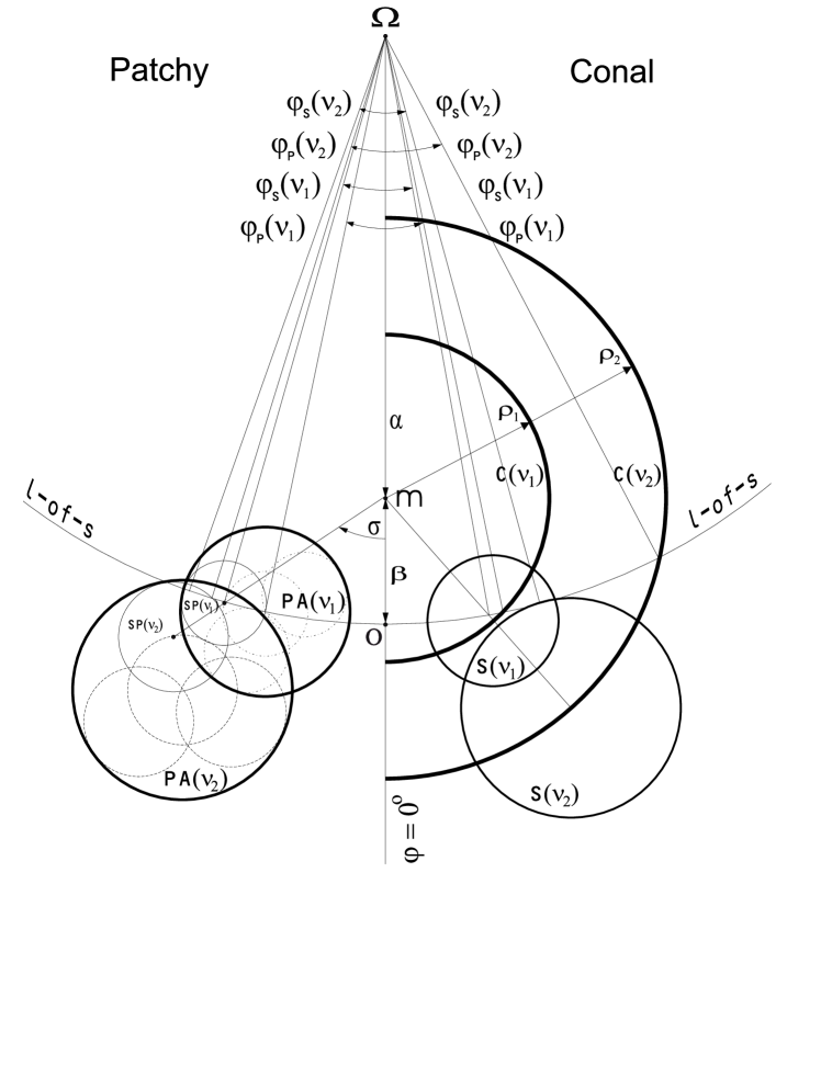
Figure 1: The beam emission patterns for both the conal model (illustrated on the right-hand side), and for the patchy beam model (illustrated on the left-hand side) are presented in this composite picture. The geometry of observation is determined in both models by the inclination angle $\alpha$ between the magnetic $\bf{m}$ and the spin $\bf\Omega$ axes and the impact angle $\beta$ of the closest approach of the line-of-sight (observer ${\bf O}$) to the magnetic axis $\bf{m}$. The fiducial plane containing the spin axis $\bf\Omega$, the magnetic axis $\bf{m}$ and the observer $\bf{O}$ defines the fiducial longitude $\varphi=0^{\circ}$ which is common for both models. All pulse phases ($\varphi_{s}$ - longitude of subpulse peak, $\varphi_{p}$ - longitude of profile component peak) are measured from this fiducial longitude, to the left from it in the patchy model and to the right from it in the conal model. In this paper we ignore the dispersive delays which are the only cause of frequency variation at or near the fiducial plane. The frequency-dependent position of any observed feature in the beam pattern is described by two angles: the opening angle $\rho(\nu)$ between the ${\bf m}$ axis and the line-of-sight (l-of-s) and by the azimuthal angle $\sigma$ between the fiducial plane and the plane of dipolar field lines associated with a particular feature. Within the conal model the subpulse emission is associated with the frequency dependent subpulse spots $S(\nu)$, which move circumpherentially to form a cone $C(\nu)$. Thus, the profile components are associated with the frequency dependent cones in the conal model, while within the patchy model the subpulse-associated spots $SP(\nu)$ occupy the patchy areas $PA(\nu)$ related to the profile components. The longitudes of subpulse peaks $\varphi_{s}(\nu)$ and profile peaks $\varphi_{p}(\nu)$ are marked, with $\nu_{1}>\nu_{2}$, in both models.

Observations of single pulses in strong pulsars show that longitudes of subpulses are weakly dependent on frequency as compared with longitudes of corresponding profile components (Izvekova et al., 1993; Gil et al., 2002). Within the conal model, the longitudes of profile components are determined by the intersection of the line of sight trajectory with the frequency-dependent cones of the maximum average intensity, while the longitudes of subpulses are determined by the intersection of the line-of-sight trajectory with subpulse-associated emission beams, which move across the average cones as frequency changes (Gil & Krawczyk, 1996). We demonstrate in this paper that the different frequency dependence of subpulse and profile component longitudes is a natural property of the conal model, and that both subpulses and profile components should demonstrate the same frequency dependence of their longitudes within the patchy model. We present both general qualitative arguments and detailed quantitative model calculations to support the above statements. For better understanding of our arguments, this paper should be studied along with the paper by Gil et al. (2002, GGGK hereafter), in which details of frequency dependence of emission patterns in PSR B0329$+$54 are discussed within the conal model of pulsar beams.

2 Geometry of pulsar radio beams

It is widely believed that narrow-band pulsar emission is relativistically beamed tangentially to dipolar magnetic field lines. Thus, the emission beaming geometry can be described by an opening angle $\rho=1^{\circ}.24\leavevmode\nobreak\ s\ r_{6}^{1/2}P^{-1/2}$, where $r_{6}=r(\nu)/R$ is the normalized emission altitude (in units of stellar radius $R=10^{6}$ cm). The mapping parameter $0\leq s=d/r_{p}\leq 1$ is determined by the locus of dipolar field lines on the polar cap ($s=0$ at the pole and $s=1$ at the polar cap edge), where $d$ is the distance from the magnetic axis $\bf{m}$ to the field line on the polar cap corresponding to a certain detail of the pulse profile (peak of subpulse or profile component), and $r_{p}=1.4\cdot 10^{4}P^{-1/2}$ cm is the canonical polar cap radius. According to the generally - accepted concept of the radius-to-frequency mapping, higher frequencies are emitted at lower altitudes $r(\nu)$ than lower frequencies. Kijak & Gil (1997, 1998) found a semi-empirical formula describing the altitude of emission region corresponding to a given frequency $\nu_{\rm GHz}$ (in GHz) which reads $r_{6}\approx 50\cdot\nu_{\rm GHz}^{-0.21}\cdot\tau_{6}^{-0.1}\cdot P^{0.33}$, where $\tau_{6}$ is the pulsar characteristic age in million years and $P$ is the pulsar period. This formula for emission altitudes is used in our model calculations.

To perform geometrical calculations of the radiation pattern one has to adopt a model of instantaneous energy distribution on the polar cap. Any specific intensity distribution can be transferred from the polar cap along dipolar field lines to the emission region, and then along straight lines (following the opening angles $\rho=1^{\circ}.24(d/r_{p})r_{6}^{1/2}P^{-1/2}$) to a given observer specified by the inclination and impact angles ($\alpha,\leavevmode\nobreak\ \beta$). We assume that at any instant the polar cap is populated by a number of features with a characteristic dimension ${\cal D}$, delivering to the magnetosphere corresponding plasma columns flowing along separate bundles of dipolar magnetic field lines. Each feature can be modelled by the Gaussian intensity distribution. Since the elementary pulsar radiation is relativistically beamed along the magnetic field lines, we can transform the feature-associated intensity pattern to the radio emission region and obtain the subpulse intensity $I$ observed at the longitude $\varphi$ in the form $I_{i}=\exp(-\kappa l_{i}^{2}(\varphi)/{\cal D}^{2})$ where the subscript $i$ lebels different features and $l_{i}^{2}(\varphi)=d^{2}(\varphi)+d_{i}^{2}-2d(\varphi)d_{i}\cdot\cos[\sigma(\varphi)-\sigma_{in}]$. Each features is located at the position (Fig. 1) described by the polar co-ordinates $d_{i}$ (distance from the pole) and $\sigma_{in}=\sigma_{io}+nD_{r}$ (magnetic azimuth angle), where the subscript $o$ refers to the initial position corresponding to the first pulse, $n$ is the sequential pulse number and $D_{r}$ is the drift rate. The instantaneous emission of the $n$-th pulse is described by $I_{n}(\varphi)=\Sigma_{i=1}I_{i}(\varphi)$, where the sum includes a number of adjacent features contributing significantly to the observed intensity, depends strongly on the inclination $\alpha$ and the impact $\beta$ angles, determining the cut of the line-of-sight tracjectory across the beam (Fig. 1). In fact, the running polar co-ordinates along the line-of-sight trajectory can be expressed in the form $d(\varphi)=[\rho(\varphi)/1^{\circ}.24]r_{p}r_{6}^{-1/2}P^{1/2}$ and $\sigma(\varphi)={\rm atan}\left\{\frac{(\sin\varphi\sin\alpha\sin(\alpha+\beta)}{\cos(\alpha+\beta)-\cos\alpha\cos\rho(\varphi)}\right\}$, and $\rho(\varphi)=2{\rm asin}\left\{\sin^{2}(\varphi/2)\sin\alpha\sin(\alpha+\beta)+\sin^{2}(\beta/2)\right\}$, (Gil et al., 1984). The average pulse profile is therefore $I(\varphi)=\frac{1}{N}\Sigma_{n=1}^{N}I_{n}(\varphi)$, where $N$ is the number of averaged single pulses. The geometry of pulsar radiation described above (for more details see Gil & Krawczyk, 1996, 1997, GGGK) can be applied to both conal and patchy beam models (Fig. 1).

We adopt a model of a pulsar beam in which the instantenous subpulse emission corresponds to a number of isolated subpulse beams, while the average emission reflects the conal structure resulting from circumferential motion of subpulse beams (Ruderman & Sutherland, 1975; Gil & Krawczyk, 1996, 1997; Gil et al., 2002). Therefore, the longitudes of subpulse peaks correspond to phases of interception of the subpulse beams by the line-of-sight trajectory, while the longitudes of profile component peaks are determined by the intersection of the line-of-sight trajectory with the average cones. The important point is that within such model the subpulse enhancements generally follow bundles of magnetic field lines different from those of enhancements corresponding to the profile components (Fig. 1 - right-hand side). On the contrary, within the patchy model both subpulse and profile component enhancements follow approximately the same bundles of field lines (Fig. 1 - left-hand side). This should be clear from the composite Fig. 1. In fact, subpulse enhancements are associated in both models with small subpulse spots $S$ following a narrow bundle of dipolar field lines, while the profile components correspond to the conical structures $C$ in the conal model, and to the narrow patches $PA$ enclosing subpulse spots in the patchy model. Because of the diverging nature of dipolar field lines controlling the plasma flow, all discussed emission features $S$ (spots), $SP$ (sub-patches), $PA$ (patches) and $C$ (cones) are frequency dependent, and two frequencies $\nu_{1}$ and $\nu_{2}$ are marked for each feature in Fig. 1.

Figure 2: Simulation of the distribution of separations $\Delta\varphi_{s}$ between subpulse peaks as compared with separation $\Delta\varphi_{p}$ between the component peaks (vertical solid lines) measured at two frequencies (400 and 1400 MHz) within the framework of the conal model (panel a) and various versions of patchy model (panels b - f). The number of pulses (out of the total number of 2000 simulated) is shown on the vertical axis and the separation in degrees of longitude is shown on the horizontal axis. The dashed vertical line going through panels b - f is shown to refer to the separation $\Delta\varphi_{p}=2^{\circ}.875$ in the pure conal model (panel a).

2.1 Conal model of pulsar beams

The frequency dependence of pulsar emission patterns within the angular beaming model of subpulse emission, and the related conal model for a mean pulsar beam is illustrated in the right-hand side of the composite Fig. 1. The subpulse-associated sub-beams corresponding to HPBW (half power beam width) of subpulse emission (thin small circles), which are called spots and marked by $S(\nu)$, perform a more or less organized circumferential motion around the magnetic axis $\bf{m}$, in which the azimuthal angle $\sigma$ varies with time, while the opening angle $\rho(\nu)$ remains constant. On average, this motion determines the cones (thick large circles) of the maximum mean intensity with the opening angles $\rho_{1}$ and $\rho_{2}$ at frequencies $\nu_{1}$ and $\nu_{2}$, respectively. The frequency-dependent longitude $\varphi_{p}(\nu)$ of the profile component is determined by the intersection of the line-of-sight with the average cone at the frequency-dependent opening angle $\rho(\nu)$. On the other hand, the frequency-dependent longitude $\varphi_{s}(\nu)$ of a subpulse peak is determined by the local maximum intensity along the cut of the line-of-sight through the subpulse spot $S(\nu)$. When the frequency changes from $\nu_{1}$ to $\nu_{2}$, the subpulse peak longitude changes from $\varphi_{s}(\nu_{1})$ to $\varphi_{s}(\nu_{2})$, while the corresponding profile peak longitude changes from $\varphi_{p}(\nu_{1})$ to $\varphi_{p}(\nu_{2})$. Note that the frequency separation $\Delta\varphi_{p}=\varphi_{p}(\nu_{2})-\varphi_{p}(\nu_{1})$ of profile peaks is generally larger than the frequency separation $\Delta\varphi_{s}=\varphi_{s}(\nu_{2})-\varphi_{s}(\nu_{1})$ of subpulse peaks. This is consistent with observations published by Izvekova et al. (1993), confirmed recently by GGGK. As we argue in the next section, within the patchy beam model $\Delta\varphi_{p}\approx\Delta\varphi_{s}$, which is quite different from the conal model in which $\Delta\varphi_{p}\stackrel{{\scriptstyle>}}{{{}_{\sim}}}\Delta\varphi_{s}$.

We now attempt to quantify our qualitative statements presented above. We use the geometrical method of transferring the instantaneous intensity distribution from the polar cap to the radio emission region along the dipolar field lines. To be able to compare the results of simulations with the observational data of PSR B0329+54 (GGGK) we adopt the following parameters $P=0.714$ s, $\dot{P}=2\cdot 10^{-15}$, $\alpha=20^{\circ}$, $\beta=4^{\circ}$, $\nu_{1}=0.4$ GHz and $\nu_{2}=1.4$ GHz. The conal model is represented by an arrangement of 12 equisized and equidistant sparks, each having the HPBW diameter ${\cal D}\sim 0.2r_{p}$, circulating around the magnetic pole at a distance of about 2/3 of the polar cap radius $r_{p}$. The results of simulations are presented in Fig. 2 (panel a). The vertical solid line at about $2.9^{\circ}$ represents the separation $\Delta\varphi_{p}$ between the peaks of the average component measured at the two frequencies. The distribution of the separations $\Delta\varphi_{s}$ of subpulse peaks measured at the two frequencies has a width of about $0.8^{\circ}$ and peaks around 1.1^∘. The apparent difference between the peak of subpulse separation and the component peak separation i.e. $\Delta\varphi_{p}-\Delta\varphi_{s}^{\rm peak}\sim 1.8^{\circ}$, as well as the width and somewhat skewed shape of the distribution, resemble the observational data quite well (see Fig.4 in GGGK, keeping in mind that zero position bin in their histograms corresponds to cases when $\Delta\varphi_{p}=\Delta\varphi_{s}$). We have taken into account only subpulses that corresponded to the same spark at both frequencies. In terms of the observational data this corresponds to subpulses correlating at two frequencies (refer to the CCF technique used in GGGK).

2.2 Patchy model of pulsar beams

Within the patchy model of pulsar beams (LM88; Manchester, 1995) the observed pulse profile is the product of a “source function” and a “window function”, which can be related to the energy/density distribution of plasma beams along different bundles of dipolar field lines and to properties of the emission mechanism, respectively. This model is illustrated schematically on the left-hand side of the composite Fig. 1. The subpulse-associated spots marked by $SP(\nu)$ corresponding to the HPBW of subpulse emission (thin small circles), occur within the limited areas $PA(\nu)$ called patches (the simplest and probably unrealistic model is when a patch $PA$ can accommodate just one sub-patch $SP$). The occurrence of $SP(\nu)$ within $PA(\nu)$ can be completely random, or more or less organized (including drifting). The dependence on frequency $\nu$ reflects the diverging nature of dipolar field lines, thus $\nu_{2}<\nu_{1}$. The bundle of field lines associated with a patch $PA(\nu)$ is only slightly larger than each bundle associated with $SP(\nu)$. This means that enhancements corresponding to subpulses and profile components follow approximately the same bundles of field lines. Thus, the frequency dependence of emission patterns in the patchy model (left-hand side of Fig. 1) should be different from that of the conal model (right-hand side of Fig. 1), in which subpulse enhancements (spots) and profile components (cones) generally follow quite different bundles of field lines. If the patch is relatively small as compared to the entire polar cap, then the frequency separation of the profile components $\Delta\varphi_{p}=\varphi_{p}(\nu_{2})-\varphi_{p}(\nu_{1})$ and that of subpulses $\Delta\varphi_{s}=\varphi_{s}(\nu_{2})-\varphi_{s}(\nu_{1})$ should be about the same. We demonstrate this below by means of geometrical simulations.

We have calculated a sequence of single pulses and average emission again for the case of PSR B0329+54, assuming that the subpatch $SP(\nu)$ is comparable in size with the spark associated emission in the conal model, and that the patch $PA(\nu)$ is twice larger than $SP(\nu)$. Thus, the projection of a patch onto the polar cap has a characteristic dimension $P\sim 2{\cal D}\sim 0.4r_{p}$. Such a patch encompasses about 30^∘ in magnetic azimuth (roughly corresponding to the scale presented in Fig.1 (left-hand side)). The results of simulations are presented in Fig. 2 (panel b). The solid vertical line at about 1^∘.25 represents the separation of the profile component associated with $PA(\nu)$ measured at the two frequencies. The narrow distribution of subpulse peak separations peaks exactly at the same value (we have again taken into account only subpulses associated with the same subpatches $SP(\nu)$ at both frequencies). It is worth noting that if we chose the sizes of $SP(\nu)$ and $PA(\nu)$ to be equal (which is the simplest and an unrealistic model of the patchy emission), the distribution would be represented by a delta function coinciding with the solid vertical line. The case presented in panel (b) is inconsistent with the frequency dependence of pulsar radiation patterns (GGGK and reference therein).

We now start to increase the azimuthal dimension of the patch $PA(\nu)$ along the cone, keeping the radial dimension the same (about 2 spark diameters ${\cal D}$ or about $0.4r_{p}$). Panels c - f in Fig. 2 correspond to the elongation factor 1.3, 1.5, 2.0 and 2.5, respectively. Thus, the maximum elongation is equivalent to the length scale comparable with the polar cap radius $r_{p}$. As one can easily notice from panels c - f, increasing elongation results in two effects: (1) the separation of the component peaks increases towards the value corresponding to the conal model (dashed vertical line) i.e $\Delta\varphi_{p}\to 3^{\circ}$, while the distribution of subpulse peak separations $\Delta\varphi_{s}$ gets broader and broader and peaks at correspondingly larger and larger distances from $\Delta\varphi_{p}$. Moreover, the skewed shape of the distribution becomes more and more apparent in panels (d) and (e), to such an extent that the case presented in panel (f) seems almost undistinguishable from the pure conal case presented in panel (a), except that the width of the distribution is too large compared with observations (see Fig. 4 in GGGK). Further increasing of the elongation factor beyond 2.5 (corresponding to 60^∘ of magnetic azimuth or 1/6 of the full cone) does not practically change the results of the simulations. This means that the unrealistic patches elongated to a large extent along circles centered on the magnetic axis would resemble the conal model. Although this conclusion seems trivial, it allows us to constrain some characteristics of both patchy and conal models. This is described in the two following paragraphs.

First we can ask: what is the probability that an adequately large and favourable patch elongated along a cone and corresponding to panel (f) mimics the conal model presented in panel (a) of Fig. 2. Of course, we have to take into account that another similar patch is required on the opposite side of the fiducial plane (see Fig.1) to account for the second outermost component of PSR B0329+54. Let us assume for simplicity that our elongated patch is a rectangular figure with the shorter side $A\approx 0.4r_{p}$ and the longer side $B\sim 1.0r_{p}$ (see above for an estimate of the dimensions). Thus, the surface area of such a patch $S_{patch}\approx A\cdot B=0.4r_{p}^{2}$ and the probability of its occurence in any location of the polar cap is ${\cal P}_{1}=S_{patch}/S_{cap}=0.4r_{p}^{2}/(\pi r_{p})^{2}\approx 0.13$. The probability of occurence of another such patch somewhere on the remaining part of the polar cap is ${\cal P}_{2}=S_{patch}/(S_{cap}-S_{patch})\approx 0.15$. To estimate the probability of the proper alignment along the cone, we can calculate a number of different independent orientations of our rectangular figure inscribed into a circle of the diameter approximately equal to $A=r_{p}$. One can easily show that the number of independent orientations is approximaly $2\pi(r_{p}/2)/(0.4r_{p})\sim 8$ and thus the probability of alignment along a cone ${\cal P}_{0}\sim 0.12$. So far, the resultant probability is ${\cal P}={\cal P}_{1}\cdot{\cal P}_{2}\cdot{\cal P}_{0}^{2}\approx 3\cdot 10^{-4}$. The requirement of having two such patches symmetricaly placed with respect to the fiducial plane only decreases the final probability. Thus, we can conclude that mimicking the conal radiation pattern by a specially arranged patchy distribution is extremly unlikely, at least in the case of PSR B0329+54 and other pulsars showing similar frequency dependence of emission patterns (GGGK and references therein).

We can now approach the results of our elongation exercise from a different angle. Since further elongation beyond the case presented in panel (f) does not change the obtained distribution, we can constrain the possible spread of the cone in the radial direction as compared with the ideal (and probably not realistic) case presented in panel (a). Remembering that the initial patch size $PA$ (panel b) was twice $SP$, with $SP$ corresponding to the spark size $\cal D$, we conclude that the realistic version of the cone can accommodate up to two sparks in radial dimension. This means that a locus of maximum intensity within the average pulsar beam has the form of a narrow ring rather than a circle.

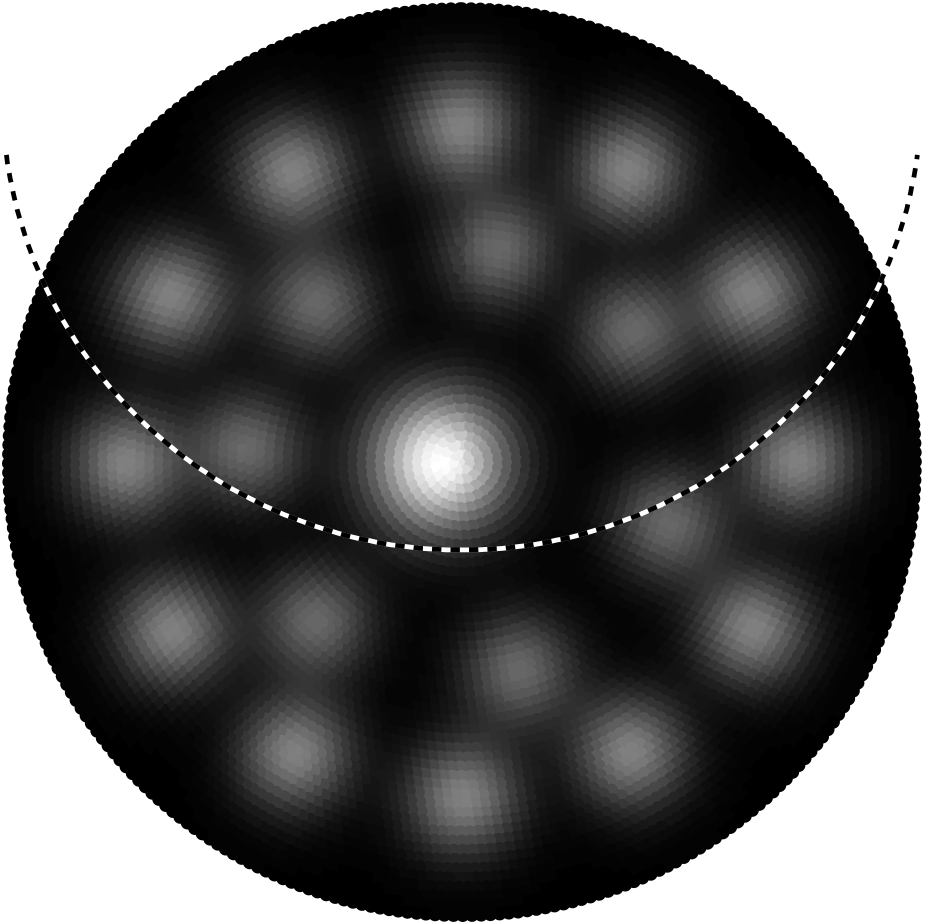
Figure 3: The proposed geometry of observation and the instantenous arrangement of sparks on the polar cap for conal model of pulsar beam of PSR J1834$-$0426. Notice that about 30% of the line-of-sight (l-of-s) trajectory covers the beam, resulting in very broad ($\sim 130^{\circ}$) profile of this pulsar.

2.3 Beam reconstruction techniques:

Recently Han & Manchester (2001; HM01 hereafter) attempted to reveal the shape of pulsar radio beams. They claim to have constructed a two-dimensional image of the “average” mean pulsar beam using a special technique applied to all available multi-component pulse profiles with good quality polarimetric data. They mapped the observed profile intensity onto the line-of-sight crossing the normalized polar cap at the normalized impact angle $\beta_{n}$ estimated from the polarization angle swing. To include a second dimension (perpendicular to the line-of-sight), they broadened the distribution in latitude applying a Gaussian to each longitudinal sample. Adding all pulsars together they obtained a global average beam pattern, which (after normalization to correct for the nonuniform distribution of $\beta_{n}$) they believe represents the global mean pulsar beam. HM01 concluded that their results are consistent with the patchy rather than conal beam model (see their Fig. 4). However, as we demonstrate in items (i)-(iv) below, their beam reconstruction technique is not general enough to reveal the true structure of pulsar beams.

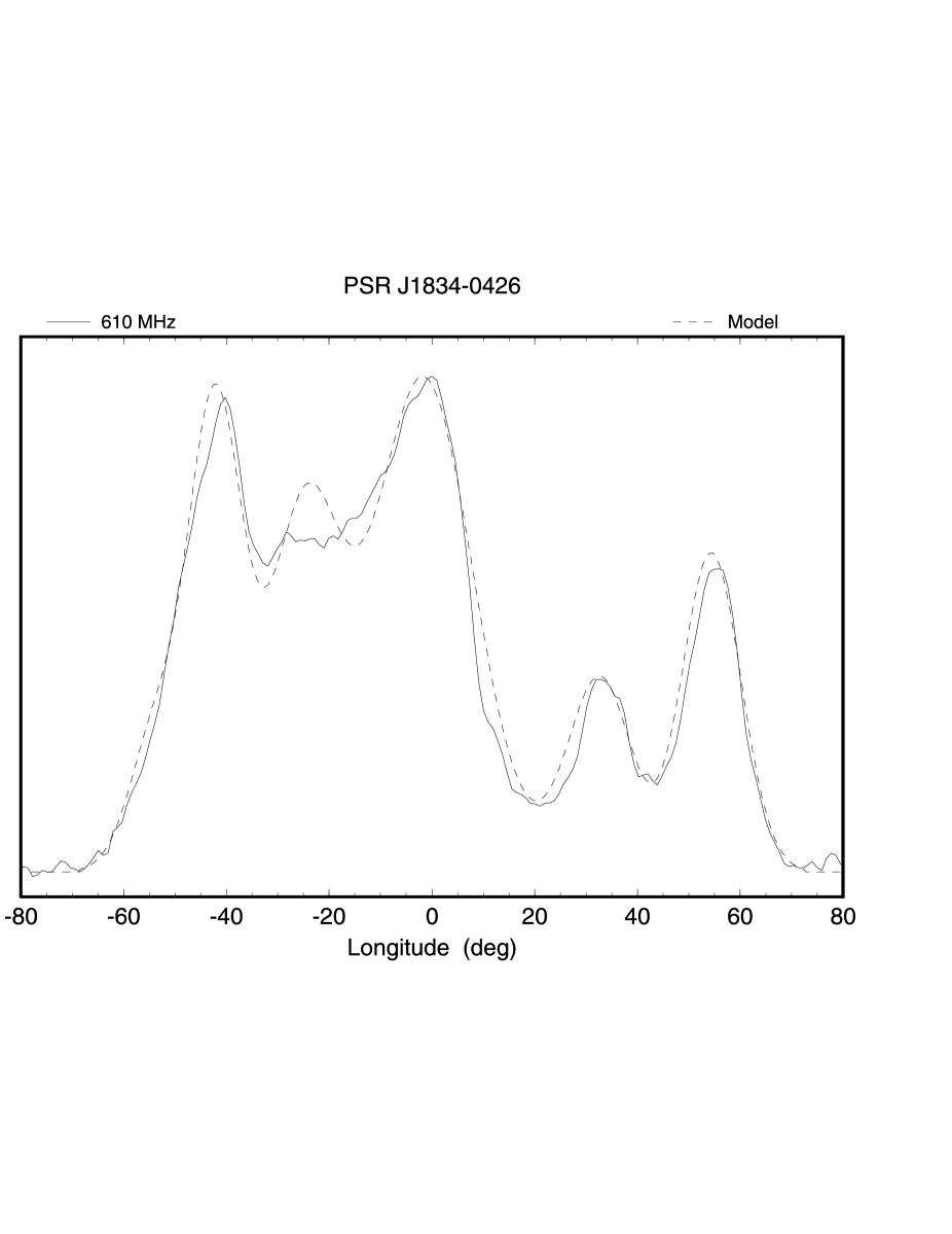
Figure 4: The observed (solid line) and simulated (dashed line) mean profile of PSR J1834$-$0426. The conal model calculations corresponding to 610 MHz were performed following the instantaneous energy distribution (presented in Fig. 3). The geometry of observations was determined by the inclination angle $\alpha=10^{\circ}$ and the impact angle $\beta=2^{\circ}.5$. The adopted emission altitude $r(610\leavevmode\nobreak\ {\rm MHz})\approx 30R$. The 610 MHz observational data (Gould & Lyne, 1998) were taken from the European Pulsar Network data base (http://www.mpifr-bonn.mpg.de/div/pulsar/data/)

(i) HM01 projected all emission features onto a normalized polar cap, ignoring the dependence of the beaming angles on the emission altitude, which most probably depends both on the radio frequency and on the pulsar period and its derivative (Kijak & Gil, 1997, 1998; Kijak, 2001). Taking into account the diverging nature of dipolar field lines with increasing altitudes, the projection of the emission pattern onto the polar cap must be performed more carefully. HM01 used data at frequencies between 600 MHz and 1.6 GHz, which probably takes care of frequency dependence of the opening angles $\rho(\nu)\propto r^{1/2}(\nu)\propto(\nu)^{-0.1}$. However, the period dependence $\rho(p)\propto P^{\sim 0.2}$ is stronger and can result in a broader spread of projections onto the normalized polar cap for short and long period pulsars, respectively.

(ii) A similar problem concerns the putative conal structure of pulsar beams which HM01 did not reject a priori. However, they assumed that adding the normalized polar caps of different pulsars would not smear the conal structure, if it existed. It seems that the conal patterns are almost certainly different in different pulsars. MD99 showed that the pulsar emission beams follow a nested cone structure with up to three distinct cones, although only one or more of the cones may be active in a given pulsar (see also Rankin, 1993; Gil et al., 1993). Also GS00 argued that the number of cones is a function of the basic pulsar parameters $P$ and $\dot{P}$.

(iii) The analysis of HM01 is based on the orthogonal normalized impact parameter $\beta_{n}=\beta_{90}/\rho_{90}$ , where $\beta_{90}$ and $\rho_{90}$ are the impact angle $\beta$ and the beam radius $\rho$ computed for the inclination angle $\alpha=90^{\circ}$ (LM88). The orthogonal normalized impact parameter $\beta_{n}$ differs from the actual normalized impact parameter $\beta/\rho$ in many aspects (e.g. Gil et al., 1993). We would like to emphasize here that $\beta/\rho$ depends on the pulsar period $P$, the inclination angle $\alpha$ and the observing frequency $\nu$. These dependences, which can affect the emission patterns, are not accounted for in the HM01 analysis based on the orthogonal impact parameter.

(iv) HM01 included the core components in their analysis. This is another possible source of confusion, since the core components are rather randomly placed with respect to the midpoint of the overall profile. For this reason MD99 excluded the core components from their analysis, which revealed a nested cone structure of pulsar beams.

Given the problems listed above, we conclude that the results of the HM01’s beam reconstruction are illusive. The lack of an apparent conal structure in their ’global’ pulsar beam does not exclude the existence of such structures in particular pulsars, expecially if they are determined by physical and geometrical factors, which may vary a great deal among different pulsars. HM01 demonstrated that the conal emission is not confined to a single region at the beam boundary. They also concluded that if multiple cones exist, they are at different radii relative to the beam radius in different pulsars. This is exactly what the multi-nested cone model of GS00 predicts. Both the number of cones and the relative radius of a given cone depend on a pulsar period and its derivative in their model.

As an example of pulsar modelling within the multi-nested cone scenario (GS00), we use the case of PSR J1834$-$0426. The patchy model for this pulsar was presented by HM01 (their Fig. 1). This pulsar has a very broad profile with the pulse width $W\sim 130$ degrees of longitude, which implies a small inclination angle $\alpha\ll 90^{\circ}$. Assuming a realistic emission altitude $r_{6}\sim 40$ (Kijak & Gil, 1997, 1998) we estimated the observational angles $\alpha\sim 10^{\circ}$ and $\beta\sim 2^{\circ}.5$ (consistent with $\alpha=7.9^{\circ}$ and $\beta=1.6^{\circ}$ given by LM88). Figure 3 shows an instantenous arrangement of sparks on the polar cap of PSR J1834$-$0426, obtained from the complexity parameter of GS00. The circumferential motion of these sparks results in the average structure of two nested cones (e.g. Fig. 6 in GGGK). Notice that about 35% of the line-of-sight trajectory stays within the beam, which leads to a broad $\sim 130^{\circ}$ average profile presented in Fig. 4.

3 Discussion and conclusions

In this paper we explore a geometrical method of pulsar radiation simulation, based on two well-justified assumptions: (i) the elementary coherent radio emission is narrow-band, and the emission altitude depends on both the frequency and the pulsar period, (ii) the emission is relativistically beamed tangently to dipolar magnetic field lines. We have considered two competitive models of the organization of pulsar emission beams: the conal model, in which enhancements related to subpulse emission in single pulses are distributed along the cones corresponding to maximum average intensity, and the patchy beam model in which subpulse enhancements corresponding to the component of the mean profile are confined to the patchy area limited both in azimuthal and radial dimensions. We examined the consistency of these rival models with the variety of observational data.

We have argued that a number of observational properties of pulsar radio emission, namely: (i) binomial distribution of the opening angles (Rankin, 1993; Gil et al., 1993; Kramer et al., 1994); (ii) high impact angles corresponding to single and double profile pulsars (MD), and (iii) different frequency dependence of a subpulse and corresponding profile component longitudes (Izvekova et al., 1993; Gil & Krawczyk, 1996; Gil et al., 2002), strongly support the conal model of pulsar beams. The alternative patchy beam model is inconsistent with these observational properties of pulsar radiation.

We have also demonstrated that the beam reconstruction technique developed by Han & Manchester (2001) is not capable of revealing the true structure of pulsar beams. In fact, their formalism assumes implicitely that neither the radio emission altitude nor the number of putative nested-cones and their locations within the pulsar depends on the pulsar period. The lack of an apparent conal structure in their ”global beam” does not exclude the conal beam model. Thus, the results of the HM01 analysis provide no strong evidence of patchy beam structure in pulsars.

We tend to favour the version of the conal model in which the relationship between the subpulse-associated beams and cones of the average emission is established through the phenomenon of the ${\bf E}\times{\bf B}$ drift (Ruderman & Sutherland, 1975; Deshpande & Rankin, 1999, 2001, GS00), which forces the spark filaments of plasma to rotate slowly around the magnetic axis. This “spark model” of radio pulsars was recently tested statistically by Fan et al. (2001). They showed, by means of Monte Carlo simulations, that various pulsar parameters can be reproduced if both the spark dimension and their mutual separation are approximately equal to the height $h$ of the polar gap (Ruderman & Sutherland, 1975, GS00), or consequently, the maximum number of sparks along the diameter of the polar cap with the radius $r_{p}$ is $N_{max}\sim r_{p}/h$. Thus, their conclusions are consistent with the assumptions used in this paper.

We note that evidence of a relationship between drifting subpulses and the conal structure of mean pulsar beams already exists in the literature. Hankins & Wolszczan (1987) examined three pulsars with triple average profiles showing subpulses drifting across the full pulse window (including the central component). They found that these pulsars are consistent with two nested cones of emission, each associated with a prominent subpulse drift. Moreover, Prószyński & Wolszczan (1986) showed that in complex profile pulsars there is a strong correlation between drifting subpulses associated with different profile components. Such correlations are natural within the ${\bf E}\times{\bf B}$ induced conal model, but inconsistent with the patchy model of pulsar beams.

Finally, we suggest that more pulsars should be observed in the single pulse, simultanenous dual frequency mode. Our simulation method illustrated and described in Fig. 2 can be adapted to the analysis of such data in order to ultimately discriminate between conal and patchy beam models in pulsars.