PX Andromedae: Superhumps and variable eclipse depth

Results of a photometric study of the SW Sex novalike PX And are presented. The periodogram analysis of the observations obtained in October 2000 reveals the presence of three signals with periods of 0$\aas@@fstack{d}$142, 4$\aas@@fstack{d}$8 and 0$\aas@@fstack{d}$207. The first two periods are recognized as ”negative superhumps” and the corresponding retrograde precession period of the accretion disk. The origin of the third periodic signal remains unknown. The observations in September-October 2001 point only to the presence of “negative superhumps” and possibly to the precession period. The origin of the “negative superhumps” is discussed and two possible mechanisms are suggested. All light curves show strong flickering activity and power spectra with a typical red noise shape. PX And shows eclipses with highly variable shape and depth. The analysis suggests that the eclipse depth is modulated with the precession period and two possible explanations of this phenomenon are discussed. An improved orbital ephemeris is also determined: $T_{\rm min}[HJD]=49238.83662(14)+0\aas@@fstack{d}146352739(11)E$.

1 Introduction

PX And is probably one of the most complicated SW Sex stars (Thorstensen et al. th91 (1991); Hellier & Robinson hel94 (1994); Still et al. still (1995)). Thorstensen et al. (th91 (1991)) reported shallow eclipses with highly variable eclipse depth and repeating with a period of $\sim$0$\aas@@fstack{d}$1463533. The authors assumed a steady-state accretion disk effective temperature distribution $T_{\rm eff}\sim r^{-3/4}$ and $q\simeq 0.46$, and adjusted the inclination and disk radius to match the width and depth of the mean eclipse. They obtained $i\simeq 73.8^{\circ}$ and $r_{\rm d}\simeq 0.6R_{L_{1}}$. No other system parameters estimations have been published and all authors used the above values. Apart from the distinctive characteristics of SW Sex stars (reviewed recently by Hellier helrev (2000)), PX And shows some other interesting peculiarities. Patterson (patt99 (1999)) reported PX And to show simultaneously “negative” and “positive” superhumps, and signals with typical periods of 4–5 days. This implies that PX And most probably possesses an eccentric and tilted accretion disk. In the view of the expected stream overflow (Hellier & Robinson hel94 (1994)) all this would result in very complex accretion structures.

In this paper we report the results of a photometric study of PX And.

2 Observations and data reduction

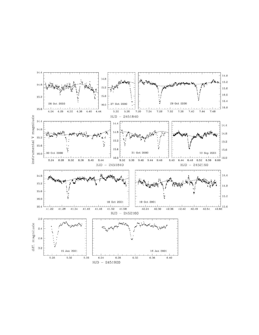
Figure 1: Observations of PX And. The best fits with the detected periods are overplotted. Note the different magnitude scale.

Photometric CCD observations of PX And were obtained with the 2.0-m telescope of Rozhen Observatory. A Photometrics 1024² CCD camera and a Johnson $V$ filter were used. The atmospheric conditions were stable with seeing $\sim$2${}^{{}^{\prime\prime}}$ and a 2$\times$2 binned camera was used. This resulted in $\sim 3$ pixels per FWHM and $\sim$13 s read-out dead-time. In total 8 runs were obtained in 2000 and 2001. The exposure time used was between 20 and 40 s. In addition, two unfiltered runs were obtained with the 1-m telescope at Hoher List Observatory. Some details of the observations are given in Table 1. After bias and flat-field corrections the photometry was done with the standard DAOPHOT aperture photometry procedures (Stetson ste (1987)). The magnitude of PX And was measured relatively to the star And1-5 ($V$=15.908) and And1-8 ($V$=16.613) served as a check (Henden & Honeycutt comp (1995)). The runs are shown in Fig. 1.

3 Results

3.1 The ephemeris

The observations cover 14 usable eclipses. The corresponding eclipse timings were determined by fitting Gaussian to the lower half of the eclipses and are given in Table 1. Combining them with the eclipse timings published by Li et al. (li (1990)), Hellier & Robinson (hel94 (1994)), Andronov et al. (andr (1994)) and Shakhvskoy et al. (shak (1995)) we determined the following orbital ephemeris:

$$T_{\rm min}[HJD]=49238.83662(14)+0\aas@@fstack{d}146352739(11)E.$$ (1)

3.2 Periodogram analysis

Table 1: CCD observations of PX And.

Date	Start	duration	mid-eclipse
	HJD-2450000	[hours]	[HJD]
Rozhen 2-m, Johnson $V$ filter
2000 Oct 26	1844.22	5.13	1844.35372
2000 Oct 27	1845.30	1.93	1845.37879:
2000 Oct 29	1847.21	7.10	1847.28135
			1847.42712
2000 Oct 30	1848.22	5.95	1848.30635
			1848.45240
2000 Oct 31	1849.33	4.50	1849.33129
			1849.47647
2001 Sep 13	2166.41	4.59	2166.47673
2001 Oct 18	2201.21	9.23	2201.30935
2001 Oct 19	2202.20	9.26	2202.33354
			2202.47930
Hoher List 1-m, unfiltered
2001 Jan 15	1925.28	1.72	1925.28667
2001 Jan 16	1926.24	3.67	1926.31250

3.2.1 Low-frequency periodicities

The mean out-of-eclipse magnitude of PX And shows large variations. The five October 2000 runs obtained within 6 nights suggest that the mean magnitude is modulated with a period of $\sim$5 days and a full amplitude of $\sim$0.5 mag. After the eclipses have been masked, the October 2000 data were searched for periodic brightness modulations by computing the Fourier transform. The complex spectral window of the data results in a power spectrum which is completely dominated by the aliases of the strong 5-days wave (Fig. 2$a$). The computed power spectrum was deconvolved with the spectral window by using the CLEAN algorithm (Roberts et al. rob (1987)). The CLEANed spectrum is shown in Fig. 2$b$. Apart from the strong low-frequency peak there are a number of peaks remaining after the cleaning. PX And has already been reported to show “negative superhumps” with a period of 0$\aas@@fstack{d}$1415 and cycles with periods of $4-5$ days (Patterson patt99 (1999); Center for Backyard Astrophysics (CBA) web site). The origin of these signals is not fully understood, but they are believed to be caused by a retrograde precession of an accretion disk which is tilted with respect to the orbital plane. In this model the relation between the orbital period $P_{\rm orb}$, the “negative superhumps” period $P^{-}_{\rm SH}$ and the precession period of the disk $P_{\rm prec}$ is given by

$$\frac{1}{P_{\rm prec}}=\frac{1}{P^{-}_{\rm SH}}-\frac{1}{P_{\rm orb}}.$$ (2)

If the peak at $P\simeq 0\aas@@fstack{d}142$ is associated with the “negative superhumps”, then the expected precession period of the disk is $\sim$4$\aas@@fstack{d}$8. Thus, the low-frequency wave seen in the data is most likely a manifestation of the disk precession. We note that CLEAN is an iterative algorithm, which is initiated with the assumption that the strongest peak in the power spectrum corresponds to a real periodicity in the data. Thus, to apply CLEAN algorithm to our PX And data we have to assume that the $\sim$5-days modulation is real. Although the baseline of our observation is short, they strongly indicate the presence of a $\sim$5-days modulation. In addition, CBA observations also reveal such a modulation. Thus, our assumption seems reasonable.

Figure 2: a–c) Periodogram analysis of the October 2000 runs. The detected periods are marked with the labelled arrows. The orbital period (the arrow without label) and the “positive superhumps” period reported by Patterson(patt99 (1999)) are also indicated. The peaks marked with “*” are artifacts from the cleaning and do not correspond to real periodicities in the data. d) Lomb-Scargle periodogram of the October 2001 runs.

To search for additional weaker signals, the $\sim$0$\aas@@fstack{d}$142 and $\sim$4$\aas@@fstack{d}$8 waves were subtracted from the data by performing a non-linear least-squares multi-sinusoidal fit with unknown amplitudes and phases. With observations over a baseline of only 6 days, $P_{\rm prec}$ could not be accurately determined; because of this $P_{\rm prec}$ was calculated from Eq. (2). The CLEANed spectrum of the residuals (not shown) shows that all strong peaks are removed. The only exception is the peak at $P\simeq 0\aas@@fstack{d}207$. The appearance of this peak is quite unusual because it could not be related to any clock in a system with $P_{\rm orb}$=0$\aas@@fstack{d}$146352739. This peak should be regarded with caution since the corresponding period is roughly equal to the mean duration of the runs. Peaks corresponding to periods of the order of the duration of the runs or harmonics of a period of 1 day may appear in the power spectrum because of the color difference between the target and the comparison star. The full amplitude of the 0$\aas@@fstack{d}$207 signal is however $\sim$0.15 mag; too large to be caused by the second-order extinction. Moreover, the second-order extinction in $V$ band is negligible. To check if this peak is not an artifact of the cleaning we applied several ways of pre-whitening. We subtracted fits with the $\sim$4$\aas@@fstack{d}$8 and $\sim$0$\aas@@fstack{d}$142 periods only, a fit with both periods but allowing them to vary in a narrow interval around peak center, etc. The results show that the peak at $P\simeq$0$\aas@@fstack{d}$207 is always present. We further estimated what is the probability for this peak to appear in the power spectrum by chance alone. This estimate is complicated by the fact that the noise in PX And light curves is red rather than white (Sec. 3.2.2). Because of this we applied the following procedure. We have generated 1000 artificial red noise time series sampled exactly as the observations, applied CLEAN to each of them and then estimated the probability to see peaks as strong as the peak at $\sim$0$\aas@@fstack{d}$207 by chance. The artificial time series were generated by the method suggested by Timmer & König (tim (1995)). This method allows one to generate random realizations of a given red noise process. The only input information needed is the power spectrum of the process. We used the mean red noise power spectrum shape derived in Sec. 3.2.2, which ensures that the artificial time series have on average the same power spectrum as the PX And light curves. The analysis of the CLEANed spectra of the artificial time series shows that the peak at 0$\aas@@fstack{d}$207 is statistically significant by more than 99%. Further, we examined whether the peak at 0$\aas@@fstack{d}$207 could be introduced in the CLEANed spectrum by the presence of the other two periodic signals, in conjunction with the red noise and the gaps in the data. To do this we added to the artificial red noise time series two sinusoids with periods of 4$\aas@@fstack{d}$8 and 0$\aas@@fstack{d}$142, and amplitudes and phases as determined from the fit of the original data. None of the CLEANed spectra of these time series show strong peaks around 0$\aas@@fstack{d}$207. This suggests that the presence of the 4$\aas@@fstack{d}$8 and 0$\aas@@fstack{d}$142 signals could not be the reason for the appearance of the 0$\aas@@fstack{d}$207 peak in the CLEANed spectrum of PX And data.

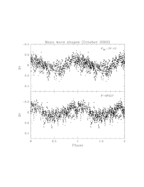
Figure 3: The October 2000 light curves folded with the 0$\aas@@fstack{d}$142 and 0$\aas@@fstack{d}$207 periods. Before the folding, the remaining two periodic signals were subtracted from the data.

In order to refine the periods we again performed a non-linear least-squares multi-sinusoidal fit to the data, but this time the periods were also allowed to vary in a narrow interval around the peaks maxima. $P^{-}_{\rm SH}$ and $P_{\rm prec}$ are not independent, so in the function used to fit the data they were coupled through Eq. (2). Thus, only $P^{-}_{\rm SH}$ and $P_{1}$=0$\aas@@fstack{d}$207 were varied. In that way the following periods were determined: $P^{-}_{\rm SH}$=0$\aas@@fstack{d}$142 $\pm$0.002, $P_{1}$=0$\aas@@fstack{d}$207 $\pm$0.004 and $P_{\rm prec}$=4$\aas@@fstack{d}$8 with semi-amplitudes of 0.086, 0.076 and 0.256 mag, respectively. The errors of $P^{-}_{\rm SH}$ and $P_{1}$ are estimated from the half-width at half-maximum of the central peak of the spectral window. A reliable error estimate of the 4$\aas@@fstack{d}$8 period is not possible mainly because the data set is short and covers only $\sim$1 cycle. The best fit is shown in Fig. 1 and the mean wave shapes of the ”negative superhumps” and 0$\aas@@fstack{d}$207 signal in Fig. 3. The CLEANed spectrum of the residuals (Fig. 2$c$) shows no peaks which implies that all peaks in the power spectrum are successfully accounted for by the fit with the detected periods.

Periodogram analysis was performed to the three runs obtained in 2001, after the subtraction of the mean of each run. The Lomb-Scargle periodogram (Scargle scar (1982)) is shown in Fig. 2$d$. The sparse distribution of the runs resulted in a complex alias structure of the periodogram. It is clear, however, that the strongest peak corresponds to a “negative superhump” with $P^{-}_{\rm SH}\simeq$0$\aas@@fstack{d}$141. This value of $P^{-}_{\rm SH}$ gives $P_{\rm prec}\simeq$3$\aas@@fstack{d}$8. The fit with these two periods is shown in Fig. 1. The corresponding semi-amplitudes are 0.069 and 0.21 mag. The 0$\aas@@fstack{d}$207 period is not detected in 2001. Note, however, that in both runs obtained on 18 and 19 October there is a slight increase of the out-of-eclipse magnitude, which might be a manifestation of a periodicity around 0$\aas@@fstack{d}$207.

Figure 4: Double logarithmic scale plot of the mean power spectrum after the subtraction of the low-frequency signals. Also shown is the best fit with Eq. (3).

3.2.2 High-frequency periodicities

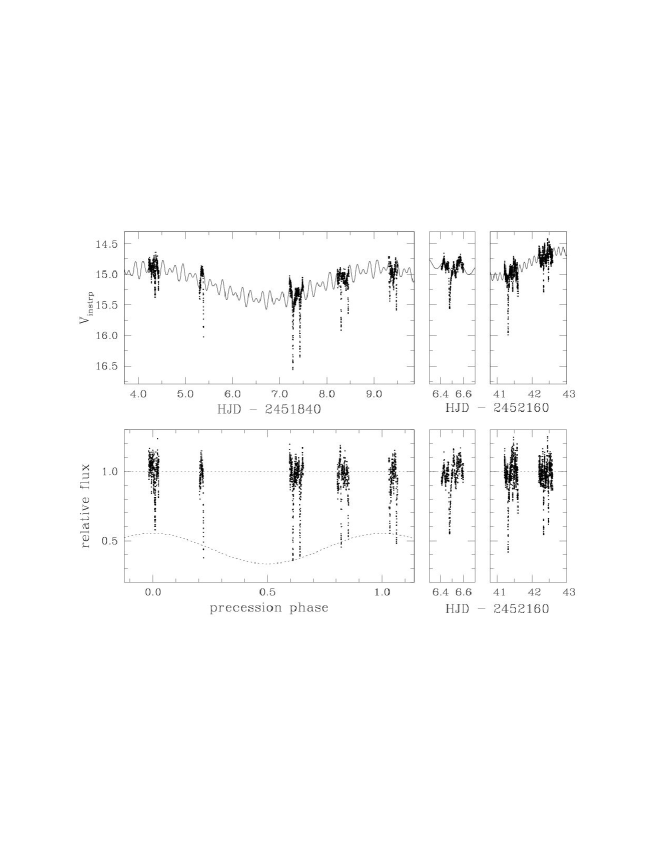
Figure 5: Upper row: $V$ band observations of PX And and the best fits with the detected periods. Lower row: The same data, but with the best fit subtracted and displayed in flux scale. The fit to the eclipse depths is also shown.

To search for high-frequency periodicities we subtracted the low-frequency signals from the data and calculated the power spectra. The periodograms show many peaks, but no coherent oscillations were detected. In double logarithmic scale the power decreases linearly with frequency (Fig. 4) and this is usually interpreted as a result of the flickering (Bruch bruch (1992)). The power spectrum can be described by the equation

$$P(f)=\frac{\alpha}{1+(2\pi\tau f)^{\gamma}}$$ (3)

with $\gamma$ being the slope of the linear part and $\tau$ may serve as an estimation of the mean duration of the dominant structures in the light curves. Equation (3) was fitted to the mean power spectrum yielding $\gamma$=1.71 and $\tau$=6 min. We also determined $\tau$ by means of autocorrelation function as described in Kraicheva et al. (1999b ). The mean value of $\tau\simeq$4 $\pm$1.5 min is slightly lower, but consistent with that determined from the fit of the mean power spectrum. The mean standard deviation in the light curves after the subtraction of the low-frequency signals is 0.061 $\pm$0.008 mag. This value is consistent with the standard deviation found in the light curves of TT Ari during the “negative superhumps” regime (Kraicheva et al. 1999a ). After switching to “positive superhumps”, the standard deviation in the TT Ari light curves decreased by a factor of 2. It would be interesting to compare this quantity in the novalikes showing only “negative” or “positive superhumps” to see if there is a systematic difference.

Figure 6: Eclipse depth as a function of the out-of-eclipse magnitude. Dots and open circles show the 2000 and 2001 data, respectively.

3.3 Variable eclipse depth

As first noticed by Thorstensen et al. (th91 (1991)) the eclipse depth in PX And is highly variable. The October 2000 runs leave the impression that the eclipse depth is modulated with the precession cycle (Fig. 5 upper row). This however could be a visual effect: the eclipses look deeper when they coincide with the superhumps minima. To verify this we have subtracted the best fit from the data and show the residuals in relative flux in the lower row of Fig. 5. The eclipse depth modulation with the precession period is evident even after the subtraction. Figure 6 shows the eclipse depth as a function of the mean out-of-eclipse magnitude. We fitted the eclipse depths with a sinusoid with the precession period. This shows that the eclipses are deepest at the minimum of the precession cycle. The mean eclipse depth is $\sim$0.56 ($\sim$0.89 mag) and the amplitude of the variation is $\sim$0.11. Thus, the eclipses we see are on average much deeper than the value of 0.5 mag reported by Thorstensen et al. (th91 (1991)). In Figs. 5 and 6 one can also find hints that in 2001 PX And was $\sim$0.2 mag brighter than in 2000.

4 Discussion

The origin of the “negative superhumps” is still an open question. The most plausible model is based on the assumption of a retrograde precession of a tilted accretion disk. While the ”positive superhumps” have been simulated numerically since the work of Whitehurst (wh (1988)), there are some difficulties to simulate the ”negative superhumps”. In fact, all attempts to simulate “negative superhumps” failed in the sense that they were not able to produce a significant tilt starting from a disk lying in the orbital plane (Murray & Armitage mur (1998); Wood et al. wood (2000)). Once tilted, however, the accretion disk starts precessing in retrograde direction (Larwood et al. lar (1996); Wood et al. wood (2000)) thus giving two additional clocks: $P_{\rm prec}$ in inertial co-ordinate system and $P^{-}_{\rm SH}$ in a system co-rotating with the binary. $P_{\rm prec}$ is typically a few days and thus $P^{-}_{\rm SH}$ is slightly shorter than the orbital period. The angle at which the accretion disk is seen from the Earth is modulated with the precession period, giving brightness modulations with $P_{\rm prec}$. Taking into account foreshortening and limb-darkening, one can estimate the disk tilt needed to produce the observed amplitude of the 4$\aas@@fstack{d}$8 modulation in PX And. With a limb-darkening coefficient $u=0.6$ the tilt angle is between 2.5^∘ and 3^∘, depending on the assumed system inclination. For comparison the simulations of Wood et al. (wood (2000)) were performed with a tilt angle of 5^∘.

Figure 7: A sketch of the system configuration at $\phi_{\rm prec}$=0.13 and $\phi_{\rm orb}$=0. The disk edge marked with the dashed line lays below the orbital plane. Also shown are the expected position of the SLS, shadow of the secondary, accretion stream and re-impact zone.

The mechanism generating the “negative superhump” light itself is however rather uncertain. According to the simulations of Wood et al. (wood (2000)) the two opposite parts of the disk which are most displaced from the orbital plane are tidally heated by the secondary. The heating is maximal when these parts point to the secondary and this happens twice per superhump cycle. Wood et al. (wood (2000)) find that the tidal stress is asymmetric with respect to the disk mid-plane and the disk surface facing the orbital plane is more heated. Thus, if the disk is optically thick the observer sees only one side and a modulation with the superhump period is observed. Let us define precession phase $\phi_{\rm prec}$ to be zero at the maximum of the 4$\aas@@fstack{d}$8 cycle, i.e. when the disk is most nearly face-on. The relative phasing between the periodic signals determined from the fit shows that the maxima of the superhumps coincide with the eclipses at $\phi_{\rm prec}\simeq$0.13. Figure 7 shows a sketch of the system configuration in eclipse at $\phi_{\rm prec}=0.13$. The expected position of the superhump light source (SLS) according to Wood et al. (wood (2000)) and the line of nodes are also shown. The dashed line marks the part of the disk which lays below the orbital plane. According to the simulations of Wood et al. (wood (2000)) the ”negative superhumps” maxima occur when the region labelled as ”SLS” in Fig. 7 lies on the line connecting the two system components, which means that the superhumps maxima will coincide with the eclipses at $\phi_{\rm prec}=0$. Our results show that in PX And this is not exactly the case and the superhumps maxima are observed $\sim 0.13P_{\rm SH}^{-}$ later.

There is another mechanism which could generate “negative superhumps” and at the same time account for the delay. Patterson (patt99 (1999)) noticed that most of the SW Sex novalikes show “negative superhumps” and this could naturally explain the accretion stream overflow thought to be responsible for the SW Sex phenomenon (Hellier & Robinson hel94 (1994)). In a system with a precessing tilted accretion disk, the amount of gas in the overflowing stream will vary with the “negative superhumps” period. Correspondingly, the intensity of the spot (shown in Fig. 7) formed where the overflowing stream re-impacts the disk should be modulated and might be the “negative” SLS. A similar model was proposed by Hessman et al. (hess (1992)) for the origin of ”positive superhumps”. The maximal overflowing is expected to take place when the most displaced part of the disk points to the accretion stream. The intensity of the re-impact spot will however reach its maximum later when the gas in the stream reaches the re-impact zone (the moment shown in Fig. 7). This means that the gas in the accretion stream which at the moment shown in Fig. 7 is near the re-impact zone, has passed over the disk edge earlier, when the system configuration was different and the most displaced part of the disk pointed to the accretion stream.

Let the gas in the overflowing stream travels from the outer disk edge to the re-impact zone in the time $\Delta t$. Then, because in co-ordinate system rotating with the binary the line of nodes precesses with period $P^{-}_{\rm SH}$, at the superhumps maxima the displaced part of the disk will not point to the accretion stream but will be rotated with respect to it by an angle $\theta\simeq 360\Delta t/P^{-}_{\rm SH}$ deg. Figure 7 shows that in the case of PX And $\theta\simeq 0.15\times 360=54^{\circ}$. Therefore, in order to observe the maxima of the “negative superhumps” at $\phi_{\rm prec}\simeq$0.13 and $\phi_{\rm orb}\simeq$0 the travel time from the outer disk edge to the re-impact zone has to be $\sim 30$ min. This is slightly longer than expected (Warner & Peters war (1972)), but we have to take into account that the velocity of the incoming gas is most probably reduced by the first impact with the accretion disk. This model for the origin of the “negative” SLS can be independently checked by tracking the intensity of the high-velocity $s$-wave observed in the spectra of SW Sex novalikes.

The origin of the 0$\aas@@fstack{d}$207 signal is quite uncertain. The corresponding peak in the power spectrum could not be a result of an amplitude modulation of the “negative superhumps”. If this is the case, the power spectrum should show two additional peaks. The secondary crosses the line of nodes twice per superhump cycle. The time between three consecutive passages coincides within 1.5% with the observed period. It is however not clear how this would produce periodic brightness modulations, moreover with the observed amplitude of $\sim$0.15 mag.

The most puzzling observation of PX And is its highly variable eclipse depth. Our observations suggest that the eclipse depth is modulated with the precession period (Figs. 5 and 6), indicating that this phenomenon could be related to the disk precession. In the precessing tilted accretion disk model, in some particular combinations of $q$ and $i$ the eclipsed area of the disk is expected to vary with the precession period and thus to modulate the eclipse depth. We have simulated eclipses of a tilted precessing disk which showed that the eclipse depth indeed varied but with a very low amplitude of 2-3%, which is insufficient to explain the observations.

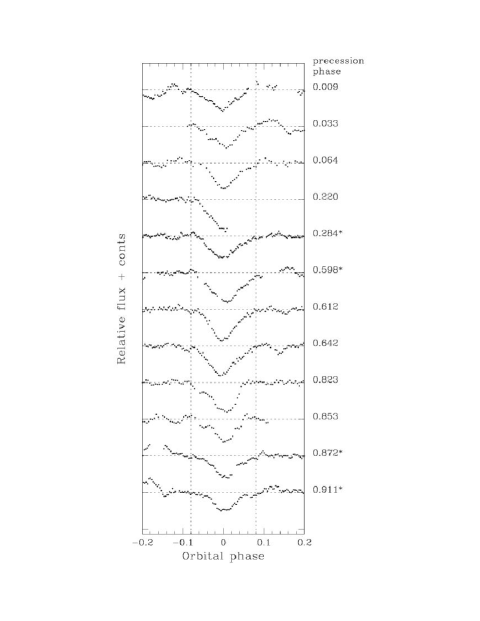
Figure 8: Normalized $V$ band eclipses of PX And. “*” mark the eclipses obtained in 2001.

The relatively shallow eclipses show that the accretion disk in PX And is not totally eclipsed. In this case, if there is a significant constant light source which is totally eclipsed, the eclipse depth will be modulated since different fraction of the total light emitted by the system will be eclipsed at different precession phases. The deepest eclipses are expected at the precession cycle minima, as observed. As the constant light source must be eclipsed, its most likely location is close to the white dwarf. The white dwarf itself could not be the source of the constant light as it does not contribute significantly to the total system light. The most obvious candidate is the inner hot part of the disk. Since the brightness modulation with the precession cycle comes from more or less pure geometrical considerations it is not clear why the emission of the inner parts of the disc could be constant. One possible explanation might be that the inner part of the disk is not tilted or is less tilted than the outer part. In this case the emission from the inner disk will be constant. Another source of the constant light could be the emission from the boundary layer between the disk and the white dwarf surface. This however is not very likely since the temperature of the boundary layer is thought to be rather high to emit significantly in the optical wavelengths. Of course, there exists the possibility that the eclipse depth modulation with the precession cycle is an artifact. If some flickering peaks occur during the eclipse (which is likely because the accretion disk in PX And is not totally eclipsed), this will decrease the observed eclipse depth. Figure 8 shows that some eclipses are indeed badly affected by the flickering. Because of the small number of eclipses covered this might introduce a spurious modulation. But since the correlation between eclipse depth and mean magnitude is good, we suggest that the eclipse depth modulation with the precession cycle is real.

Figure 9: Eclipse depth as a function of $F_{\rm mod}/F_{\rm const}$ (see text for details). Dots and open circles show the 2000 and 2001 data, respectively.

There is another way to modulate the eclipse depth. As the SLS is non-uniformly distributed over the disk surface and the accretion disk is not totally eclipsed, there are two extreme possibilities when the SLS is (i) totally and (ii) never eclipsed. In both cases the eclipse depth will depend on the actual superhump light at the moment of eclipse, but will have opposite behavior. If the SLS is totally eclipsed, then the deepest eclipses will be observed when superhump maxima coincide with the eclipses. If the SLS is never eclipsed, the eclipse depth will be affected in a way analogous to the veiling of the absorption lines in T Tau stars. In these stars the additional emission in the continuum reduces the observed depth of the absorption lines. Then the eclipses will be deepest when superhump minima coincide with the eclipses. Using the parameters of the periodic signals obtained from the multi-sinusoidal fit, we calculated the total contribution of the modulated part of the flux to the unmodulated one, $F_{\rm mod}/F_{\rm const}$, at the moments of the eclipses. $F_{\rm const}$ is modulated with the precession cycle and hence may be thought to be constant on the superhump time scale. The $\sim$0$\aas@@fstack{d}$207 signal was included in the calculations for 2000. The reason is that the eclipse depth variation observed in the 2000 data is rather high to be explained if only the “negative” SLS is involved. Figure 9 shows the eclipse depth $d_{\rm e}$ as a function of $F_{\rm mod}/F_{\rm const}$. Although the scatter is large, one should keep in mind that any flickering near the mid-eclipses will decrease the eclipse depth and will move the points in Fig. 9 downward. If a small number of eclipses are observed then this could easily obscure any correlation. Despite the large scatter, there are some hints of an inverse correlation in Fig. 9. This suggests that the SLS is not eclipsed. In Fig. 9 is also shown an arbitrary curve defined by the equation:

$$d_{\rm e}=\frac{d_{\rm e,0}}{1+F_{\rm mod}/F_{\rm const}}$$ (4)

which gives the eclipse depth as a function of the additional modulated light in the case when this light is not eclipsed. Here, $d_{\rm e,0}$ is the eclipse depth if $F_{\rm mod}=0$.

Although mathematically the veiling could explain the eclipse depth changes, there are many uncertainties with this interpretation. Most of them are related to the unknown place of origin of the periodic signals. If the conclusion of Wood et al. (wood (2000)) about where the “negative superhumps” are generated is correct, then the “negative” SLS should be at least partially eclipsed. This suggests that the stream overflow could be the mechanism generating the “negative superhumps” in PX And. Moreover, in a system with grazing eclipses the re-impact zone is not eclipsed. Apart of this, the origin of the $\sim$0$\aas@@fstack{d}$207 signal is unknown and it is not clear if its source is eclipsed or not. Thus, the question why the eclipse depth in PX And varies remains open and we have only pointed to some of the possible explanations.

Thorstensen et al. (th91 (1991)) have estimated $q$, $i$ and the disk radius of PX And by fitting a mean eclipse. It should be noted however that the observations of Thorstensen et al. (th91 (1991)) point to an average eclipse depth of $\sim 0.5$ mag while our observations show much deeper eclipses. It is clear that the highly variable shape and depth of eclipses could affect significantly any attempt to estimate the system parameters of PX And. Because of this we have not attempted such an estimation from the eclipse profiles. It would also not be correct to define so called ”mean” eclipse and to analyze it with the eclipse mapping technique. Moreover, a large part of the accretion disk in PX And is not eclipsed. The eclipse mapping algorithm could be easily modified to allow analysis of tilted accretion disks. To use this technique however one will need to average at least several eclipses at given precession phase in order to reduce the influence of flickering and other noise.

Generally, if a given cataclysmic variable shows “positive superhumps” one could estimate $q$ using the existing $\epsilon^{+}(q)$ relations ($\epsilon^{+}=(P_{\rm sh}^{+}-P_{\rm orb})/P_{\rm orb}$). Patterson (patt99 (1999)) reported that PX And shows “positive superhumps” with $\epsilon^{+}\simeq$0.09 and this could be used to estimate $q$. Recently, Montgomery (mon (2001)) published an analytic $\epsilon^{+}(q)$ expression which takes into account the pressure effect. Applying this relation (Eq. (8) in Montgomery mon (2001)) to PX And we obtain $q\simeq$0.27. Although this value of $q$ is more plausible for a system showing ”positive superhumps”, one should keep in mind that the peak in the power spectrum of the CBA data is very weak. The ”negative superhumps” are much more confidently detected, but unfortunately an $\epsilon^{-}(q)$ relation for the ”negative superhumps” has not been established yet. Patterson (patt99 (1999)) noticed that $\epsilon^{-}\simeq-0.5\,\epsilon^{+}$. Our periodogram analysis yields $\epsilon^{-}\simeq-0.029$, hence $\epsilon^{+}\simeq 0.058$. From Montgomery (mon (2001)) relation, one obtains $q\simeq 0.18$. This is not an unrealistic value but we cannot be sure that the relation $\epsilon^{-}\simeq-0.5\,\epsilon^{+}$ holds true for PX And.

Based on the analysis of our new photometric observations and on the results of Patterson (patt99 (1999)) we can with no doubt place the novalike PX And among the cataclysmic variables showing permanent ”negative superhumps”. The observations of the star in 2000 show two unusual features: the presence of another superhump with a period of $\sim$0$\aas@@fstack{d}$207 and a modulation of the eclipse depth with the precession period of the accretion disk. Our 2001 observations are however limited in time coverage and it is difficult to say if these two phenomena are typical of the star or are a peculiarity of this particular data set only. As a suggestion for future work we recommend performing a multi-site photometric observations covering several precession cycles. If the modulation of the eclipse depth with the precession period is confirmed, this phenomenon could be further studied by analysis of the eclipse profiles at different precession phases.

- (1) Andronov, I.L., Borisov, G.V, Chinarova, L.L, et al. 1994, Odessa Astronomical Publications 7, 166
- (2) Bruch, A. 1992, A&A 266, 237
- (3) Hellier, C., & Robinson, E.L. 1994, ApJ Lett. 431, 107
- (4) Hellier, C. 1998, PASP 110, 420
- (5) Hellier, C. 2000, NewAR 44, 131
- (6) Henden, A.A., & Honeycutt, R.K. 1995, PASP 107, 324
- (7) Hessman, F.V, Mantel, K.-H., Barwing, H., & Schoembs, R 1992, A&A 263, 147
- (8) Kraicheva, Z., Stanishev. V., Genkov, V., & Iliev L 1999a, A&A 351, 607
- (9) Kraicheva, Z., Stanishev, V., & Genkov, V. 1999b, A&AS 134, 263
- (10) Larwood, J.D., Nelson, R.P., Papaloizou, J.C.B., & Terquem, C. 1996, MNRAS 282, 597
- (11) Li, Y., Jiang, Zh.-J., Chen, J.-Sh., & Wei, M. Zh. 1990, IBVS 3434
- (12) Montgomery, M.M. 2001, MNRAS 325, 761
- (13) Murray, J.R., & Armigate, P.J. 1998, MNRAS 300, 561
- (14) Patterson, J. 1998, PASP 110, 1132
- (15) Patterson, J. 1999, in: Disk Instabilities in Close Binary Systems. 25 Years of the Disk-Instability Model, Proceedings of the Disk-Instability Workshop held on 27-30 October, 1998, Kyoto, Japan. Edited by S. Mineshige and J. C. Wheeler. Frontiers Science Series No. 26. Universal Academy Press, Inc., p.61
- (16) Roberts, D., Lehár, J., & Dreher, J. 1987, AJ 93, 963
- (17) Shakhvskoy, N.M, Kolesnikov, S.V., & Andronov, I.L 1995, in: Cataclysmic Variables, Proceedings of the conference held in Abano Terme, Italy, 20-24 June 1994 Publisher: Dordrecht Kluwer Academic Publishers, Edited by A. Bianchini, M. della Valle, and M. Orio. Astrophysics and Space Science Library, Vol. 205, p.187
- (18) Scargle, J.D. 1982, ApJ 263, 835
- (19) Stetson, P. 1987, PASP 99, 191
- (20) Still, M.D., Dhillon, V.S., & Jones, D.H.P. 1995, MNRAS 273, 863
- (21) Thorstensen, J.R., Ringwald, F.A., Wade, R.A., Schmidt, G,D., & Norsworthy, J.E. 1991, AJ 102, 272
- (22) Timmer, J., & König, M. 1995, A&A 300, 707
- (23) Warner, B., & Peters, W. 1972, MNRAS 160, 15
- (24) Whitehurst, R. 1988 MNRAS 232, 35
- (25) Wood, M.A., Montgomery, M.M., & Simpson, J.C. 2000, ApJ Lett. 535, 39