The REFLEX Galaxy Cluster Survey VII: $\Omega_{m}$ and $\sigma_{8}$ from cluster abundance and large-scale clustering

For the first time the large-scale clustering and the mean abundance of galaxy clusters are analysed simultaneously to get precise constraints on the normalized cosmic matter density $\Omega_{m}$ and the linear theory RMS fluctuations in mass $\sigma_{8}$. A self-consistent likelihood analysis is described which combines, in a natural and optimal manner, a battery of sensitive cosmological tests where observational data are represented by the (Karhunen-Loéve) eigenvectors of the sample correlation matrix. This method breaks the degeneracy between $\Omega_{m}$ and $\sigma_{8}$. The cosmological tests are performed with the ROSAT ESO Flux-Limited X-ray (REFLEX) cluster sample. The computations assume cosmologically flat geometries and a non-evolving cluster population mainly over the redshift range $0<z<0.3$. The REFLEX sample gives the cosmological constraints and their $1\sigma$ random errors of $\Omega_{m}\,=\,0.341\,^{+0.031}_{-0.029}$ and $\sigma_{8}\,=\,0.711\,^{+0.039}_{-0.031}$. Possible systematic errors are evaluated by estimating the effects of uncertainties in the value of the Hubble constant, the baryon density, the spectral slope of the initial scalar fluctuations, the mass/X-ray luminosity relation and its intrinsic scatter, the biasing scheme, and the cluster mass density profile. All these contributions sum up to total systematic errors of $\sigma_{\Omega_{m}}=^{+0.087}_{-0.071}$ and $\sigma_{\sigma_{8}}=^{+0.120}_{-0.162}$.

1 Introduction

Several observational arguments suggest that we live in a geometrically flat Universe in a phase of accelerated cosmic expansion (Riess et al. 1998, Perlmutter et al. 1999, Stompor et al. 2001, Netterfield et al. 2002, Pryke et al. 2002, Sievers et al. 2002). Strong indications for a low cosmic matter density come from, e.g., the abundance of galaxy clusters (e.g., Carlberg et al. 1996, Viana & Liddle 1996, Bahcall & Fan 1998, Eke et al. 1998, Henry 2000, Borgani et al. 2001, Reiprich & Böhringer 2002, hereafter RB02), and from the large-scale distribution of clusters (e.g. Collins et al. 2000, Schuecker et al. 2001, hereafter Paper I) and galaxies (e.g., Percival et al. 2001, Szalay et al. 2001). A recent overview including also new results on gravitational dynamics, weak lensing and the baryon mass fraction in clusters of galaxies can be found in Peebles & Ratra (2002).

With the present investigation we are improving the constraints on the matter density $\Omega_{m}$ and the linear theory RMS matter fluctuations $\sigma_{8}$ in comoving spheres with $8\,h^{-1}\,{\rm Mpc}$ radius. We base our approach on observational estimates of spatial clustering and abundance of galaxy clusters. Simultaneous constraints on $\Omega_{m}$ and $\sigma_{8}$ are derived under the assumption of a flat geometry of the Universe. Cluster abundances although almost insensitive to the cosmological constant $\Omega_{\Lambda}$ are known to be quite sensitive to $\Omega_{m}$ and actually one of the best ways of measuring $\sigma_{8}$ (White et al. 1993, Eke et al. 1996, Kitayama & Suto 1997, Borgani et al. 1997, Mathiesen & Evrard 1998). Our method uses the statistical information of the present epoch large-scale structure to characterize the cosmological model. In comparison to other methods of the assessment of the large-scale structure e.g. through the galaxy distribution, the analysis of the galaxy cluster distribution has the advantage that it relies on astrophysics mostly governed by gravitation, so that cluster masses and biasing factors can be obtained from first principles, especially when the clusters are selected in X-rays (e.g., Borgani & Guzzo 2001).

We use the ROSAT ESO Flux-Limited X-ray (REFLEX) galaxy cluster sample. In the REFLEX survey special care was taken to get a well-controlled sample selection and a high completeness (Böhringer et al. 2001). The sample consists of the 452 X-ray brightest southern clusters with redshifts mainly below $z=0.3$, selected in X-rays from the ROSAT All-Sky Survey (RASS, Voges et al. 1999) and is confirmed by extensive optical follow-up observations within a large ESO Key Programme (Böhringer et al. 1998, Guzzo et al. 1999). The sample has been used to measure with unrivalled accuracy the cluster X-ray luminosity function (Böhringer et al. 2002), the spatial cluster-cluster correlation function (Collins et al. 2000), and its power spectrum (Paper I).

In order to get accurate constraints on $\Omega_{m}$ and $\sigma_{8}$ we use several independent cosmological tests based on the dependence of the cosmic matter power spectrum and the volume on the values of the cosmological parameters. On the one side we measure the spatial fluctuations of galaxy clusters. This test is known to be especially sensitive to the shape of the matter power spectrum on large scales. On the other side we measure the average abundance of clusters. This test is known to be especially sensitive to the normalization of the matter power spectrum on small scales. Finally and independent from the matter power spectrum, we count clusters to measure their abundance as a function of redshift and thus to measure the volume which again strongly depends on cosmology (redshift-volume test, e.g., Robertson & Noonan 1968).

A natural way to combine the different tests is offered by the Karhunen-Loéve (KL) eigenvector analysis. The method was first applied by Bond (1995) to analyse cosmic microwave background (CMB) temperature maps and translated by Vogeley & Szalay (1996) to the case of the spatial analysis of galaxies. The KL eigenvectors $\Psi$ are constructed in a way to obey orthogonality properties which allow unbiased studies of fluctuations up to the largest scales covered by a survey. The method avoids artifical correlations introduced by the survey window between different fluctuation modes, affecting under realistic conditions all power spectral analyses based on plane-wave expansions on large scales. Applications of the KL method to galaxy surveys can be found in Matsubara, Szalay & Landy (2000) and Szalay et al. (2001). Their KL tests are, however, still restricted to the analysis of the clustering properties of galaxies.

To determine a precise eigenvector base $\Psi$ which does not bias the final results, a more refined fiducial cosmological model has to be assumed which is already close to our best model fits (the construction of the fiducial model is described in Sect. 4): a pressure-less spatially flat Friedmann-Lemaître model, the cosmic matter density $\Omega_{m}=0.3$, the cosmological constant $\Omega_{\Lambda}=0.7$, the Hubble constant in the form $h=H_{0}/100\,{\rm km}\,{\rm s}^{-1}\,{\rm Mpc}^{-1}=0.7$, the linear RMS normalization $\sigma_{8}=0.75$, the spectral index of initial scalar fluctuations $n_{\rm S}=1.0$, the baryon density $\Omega_{b}h^{2}=0.020$, and the CMB temperature $T_{\rm CMB}=2.728$ K.

In our first KL study of the REFLEX sample we followed the approach of A. Szalay and collaborators, applying the KL method to the analysis of three-dimensional spatial fluctuations (Schuecker et al. 2002, hereafter Paper II). The resulting constraints on the matter density, $0.03<\Omega_{m}h^{2}<0.19$ (95% confidence interval), were found to be quite robust against major changes in the model assumptions.

The present investigation completes our previous KL study by utilizing now both the spatial fluctuations of galaxy clusters and their mean abundance to get constraints on $\Omega_{m}$ and $\sigma_{8}$. Some general features of the KL method relevant for the present work are outlined in Sect. 2. In Sect. 3 we briefly describe a model for the matter and cluster power spectrum already developed in Paper II. We further introduce a new theoretical model for the average cluster abundance which replaces the more phenomenological prescription used in Paper II. The REFLEX sample and the values of important model parameters are discussed in Sect. 4. Sect. 5 summarizes the cosmological constraints obtained with the REFLEX sample. In Sect. 6 we discuss the results and draw our basic conclusions. In the Appendix we derive equations used to relate cluster masses defined for different density contrast and background levels.

2 General method

Clusters of galaxies are counted in cells. The results are summarized in a vector $\@vec{D}$ with elements containing the counts obtained within the individual cells. Similarily, a second vector $\@vec{N}$ is introduced which contains the average (expected) model counts. The latter are the diagonal elements of a noise matrix $N$. After the equalization of the different noise in the cells by $N^{-1/2}$ (whitening) and the KL transformation into the $\Psi$ vectorbase, the values of the cosmological parameters are estimated by minimizing the differences $\Delta\@vec{B}\,=\,\@vec{B}\,-<\@vec{B}>$ between the KL coefficients $\@vec{B}\,=\,\Psi^{\rm T}\,N^{-1/2}\,\@vec{D}$ determined by the observed sample, and the expected KL coefficients $<\@vec{B}>\,=\,\Psi^{\rm T}\,N^{+1/2}$ determined by a cosmological model (see Paper II), where T denotes the transpose of a matrix.

More specifically, the columns of the unitary matrix $\Psi$ are the KL eigenvectors of the so-called whitened correlation matrix $R^{\prime}\,=\,N^{-1/2}\,R\,N^{-1/2}$, with the elements of $R$ given by $R_{ij}\,=\,N_{i}\,N_{j}\xi_{ij}\,+\,\delta_{ij}N_{i}$ and $\xi_{ij}\,=\,\frac{1}{V_{i}\,V_{j}}\,\int_{V_{i}}d^{3}\@vec{r}_{i}\,\int_{V_{j}}d^{3}\@vec{r}_{j}\,\xi(|\@vec{r}_{i}-\@vec{r}_{j}|)$. Here, $\xi$ is the cluster correlation function, and $V_{i}$ the volume of the $i$-th count cell centered at the comoving coordinate $\@vec{r}_{i}$.

The elements of $\Delta\@vec{B}$ show random cell-to-cell fluctuations caused by both the Poisson count noise and the large-scale distribution of the clusters. For the correct weighting of $\Delta\@vec{B}$ these fluctuations are taken into account. Note that the analysis of the fluctuations alone already gives useful cosmological constraints as described in our first KL analysis (Paper II).

A simple way to perform the minimization which also utilizes the cosmological information contained in the random fluctuations between the cells is suggested by the observed frequency distribution of the KL coefficients. For the REFLEX cluster survey we found (Paper II) that for large cell sizes, $\@vec{B}$ follows a Gaussian distribution with high statistical significance (new results are given in Fig. 6 of the present paper). A multivariate sample likelihood function of an assumed cosmological model should thus have the form

$${\cal L}(\@vec{B}|\@vec{x})\,=\,\frac{\exp\left[-\frac{1}{2}\,{\rm trace}\left(C^{-1}Z\right)\right]}{\sqrt{(2\pi)^{M}|{\rm det}C|}}\,,$$ (1)

with the sample covariance matrix $Z=\Delta\@vec{B}(\Delta\@vec{B})^{\rm T}$, the model covariance matrix of the KL coefficients $C\,=\,\Psi^{\rm T}\,R^{\prime}_{\rm model}\,\Psi$, and the parameter vector $\@vec{x}$ specifying the cosmological model. We assume as usual that the maximum of (1) determines the values of the model parameters which yield the highest probability of obtaining cluster abundances and fluctuations as large as observed. Note that in Paper II, $Z$ was fixed by a phenomenological background model (independent from any cosmological parameter) and only $C$ was regarded as a free model-dependent variable. In the present investigation both $Z$ and $C$ are computed with observed and modelled data in a consistent manner (see Sec. 3).

                                                                      

Figure 1: Likelihood contours ($1$-$3\sigma$ levels for two degrees of freedom) for models with $h=0.64$ (left) and $h=0.80$ (right). The remaining values of the cosmological parameters and model assumptions are the same as for the reference KL solution described in the main text (see also Table 1). Small stars mark the parameter values with the highest likelihoods.

                                                                      

Figure 2: Likelihood contours for models with $n_{\rm S}=0.9$ (left) and $n_{\rm S}=1.1$ (right). The values of the other parameters are given in Table 1.

                                                                      

Figure 3: Likelihood contours for models with $\Omega_{b}h^{2}=0.018$ (left) and $\Omega_{b}h^{2}=0.026$ (right). The values of the other parameters are given in Table 1.

                                                                      

Figure 4: Likelihood contours for biasing models of Sheth & Tormen (1999, left) and of Kaiser (1984, right). The former model yields the adopted reference solution. The values of the other parameters are given in Table 1.

                                                                      

Figure 5: Likelihood contours for mass/X-ray luminosity relations with $A=-20.055$, $\alpha=1.652$, $\sigma_{\rm eff}=19\%$ (left) and $A=-18.320$, $\alpha=1.538$, $\sigma_{\rm eff}=25\%$ (right); definition of $A$ and $\alpha$ as in RB02. The values of the other parameters are given in Table 1.

3 Model specifications

We briefly outline the model for the observed cluster power spectrum $P_{\rm obs}(k)$ described in more detail in Paper II and a new model for the average cluster abundance $\@vec{N}$ which replaces the empirical approach used in Paper II.

The Gaussianity of the KL coefficients $\@vec{B}$ measured with the REFLEX clusters on large scales together with the linearity of the KL transform suggest that the large-scale cosmic matter distribution is Gaussian as well and can thus be characterized by a (linear theory) matter power spectrum $P(k)$. We assume adiabatic scalar perturbations and a cold dark matter (CDM) plus baryon fluid as suggested by the observed power spectrum of CMB anisotropies (see recent CMB measurements mentioned in Sect. 1). The resulting $P(k)$ is determined by the transfer function $T_{x}(k)$, the spectral index $n_{\rm S}$ of the initial scalar fluctuations, and the normalization parameter $\sigma_{8}$. The corresponding transfer functions of Eisenstein & Hu (1998) are used, providing a more accurate description of the linear theory power spectrum than fitting equations of the kind given in Bardeen et al. (1986). Note that the $\sigma_{8}$ as introduced here reflects the amplitude of the power spectrum without any non-linear corrections.

Generally, $P_{\rm obs}(k)$ is an average over evolving matter power spectra and clusters with different values of the biasing parameter $b$. We summarize this using the prescription of Matarrese et al. (1997) and Moscardini et al. (2000). Note that the prescription implies that the observed mass and redshift-averaged cluster power spectrum has the same shape, i.e., functional form as the underlying matter power spectrum. In order to illustrate the sensitivity of the results to the biasing model we use for $b$ alternatively the model of Sheth & Tormen (1999) and Kaiser (1984). We verified the model of $P_{\rm obs}(k)$ (see Paper II) with a large set of cluster samples extracted from the Hubble Volume Simulations (e.g., Evrard et al. 2002 and the references given therein).

For the average cluster abundances the following model is used. For an unclustered distribution, the average number of clusters expected in a small cell centered at Right Ascension $\alpha$, Declination $\delta$, and redshift $z$, per unit redshift and solid angle $\omega$ is

$$\frac{dN(\alpha,\delta,z)}{dz\,d\omega}\,=\,\frac{c\,r^{2}(z)}{H(z)}\,\int_{M_{\rm lim}(\alpha,\delta,z)}^{\infty}\,dM\,\frac{dn(M,z)}{dM}\,,$$ (2)

with the usual notation $H(z)\,=\,H_{0}\,E(z)$ and $r(z)\,=\,c/H_{0}\int_{0}^{z}E^{-1}(z^{\prime})dz^{\prime}$. The average number of clusters expected in a KL cell thus is $N_{i}\,=\,\int_{V_{i}}dN$. Recent CMB measurements strongly suggest a flat space (see Sect. 1) so that $E^{2}(z)\,=\,\Omega_{m}(1+z)^{3}+\Omega_{\Lambda}$. The mass limit $M_{\rm lim}$ is obtained from the X-ray luminosity limit $L_{\rm min}$ at a given $(\alpha,\delta,z)$ and the empirical mass/X-ray luminosity relation of RB02 including its intrinsic scatter (see Sect. 4). They measured the masses within a radius with the average density contrast 200 related to the zero-redshift critical density $\rho_{c}$, assuming an Einstein-de Sitter (EdS) geometry.

For cosmological tests a mass function $dn/dM$ is needed which is form-invariant under different cosmologies. Jenkins et al. (2001) found from numerical simulations that

$$\frac{dn(M,z)}{dM}\,=\,-0.315\,\frac{\bar{\rho}(z)}{M}\,\frac{1}{\sigma(M)}\,\times$$

$$\hskip 35.56593pt\left|\frac{d\sigma(M)}{dM}\right|\,\exp\left\{-\left|0.61-\ln\left[\sigma(M,z)\right]\right|^{3.8}\right\}$$ (3)

obeys this invariance property when the masses $M$ are defined by a spherical overdensity of $18\pi^{2}$ related to the background matter density $\bar{\rho}=\Omega_{m}\,\rho_{c}$. The growth of cosmic structures introduces a redshift-dependent $\sigma$ in the mass function, giving the standard deviation of the matter density field smoothed by a spherical top-hat filter with the radius $R=[2GM/\Omega_{m}H^{2}]^{1/3}$.

In order to combine the empirical mass/X-ray luminosity relation and the mass function, two transformations of cluster masses are necessary which are described in Sect. 4 and Appendix A. Any change of the values of cosmological parameters thus changes both the observed mass/X-ray luminosity relation and the theoretical mass function. Note that the cosmology dependence of the observed mass/X-ray luminosity relation of RB02 results mainly in a change to the model-dependent virial radius, whereas for a fixed radius the dependence is significantly smaller.

4 The REFLEX sample and the values of important model parameters

The KL analysis is performed with a subsample of 426 clusters of the 452 REFLEX clusters. The clusters of the subsample are selected according to the following criteria. They are located within comoving distances $r\leq 1.0\,h^{-1}\,{\rm Gpc}$ ($z\leq 0.365$). The clusters have at least 10 X-ray source counts detected in the ROSAT energy band 0.5-2.0 keV, X-ray luminosities $L_{\rm X}\geq 2.5\times 10^{42}\,h^{-2}\,{\rm erg}\,{\rm s}^{-1}$ and X-ray fluxes $S_{\rm X}\geq 3.0\times 10^{-12}\,{\rm erg}\,{\rm s}^{-1}\,{\rm cm}^{-2}$ in the energy band $0.1$-$2.4$ keV. The clusters are located in an area of 4.24 sr in the southern hemisphere with Declination $\leq 2.5$ deg, excluding galactic latitudes $|b|\leq 20$ deg and some additional crowded fields like the Magellanic Clouds. More information about the sample construction can be found in Böhringer et al. (2001).

Several tests with observed and simulated data suggest that the REFLEX sample is at least 90% complete up to the lower X-ray luminosity limit given above (Böhringer et al. 2001, Schuecker et al. 2001). In the computation of the X-ray luminosities a $\beta$-model based correction is applied to correct the observed flux for the missing flux outside the observational apperature radius. The correction is on average about 10% and the correction procedure has been tested with Monte-Carlo simulations (Böhringer et al. 2002). For the cosmic $K$-corrections we use a refined Raymond-Smith code, where the X-ray temperatures $T_{\rm X}$ are estimated with the $L_{\rm X}$-$T_{\rm X}$ relation of Markevitch (1998) without ‘cooling flow’ corrections (ignoring higher-order effects caused by the fact that the latter relation was obtained for non-total X-ray luminosities).

For the transformation of the X-ray luminosity limit $L_{\rm min}(z)$ to the corresponding mass limit defined within an EdS geometry (see Sect. 3) the empirical mass/X-ray luminosity relation of RB02 is used with the particular parameter values $A=-20.055$ and $\alpha=1.652$ (following their notation). They measured the masses of 106 galaxy clusters with redshifts generally below $z=0.1$ mainly with ROSAT PSPC pointed observations and gas temperatures as published mainly from ASCA observations (assuming spherical symmetry, isothermality and hydrostatic equilibrium). The sample is large enough to give a statistically representative summary of the local mass/X-ray luminosity relation of massive clusters and a rough but useful estimate of its intrinsic scatter (see below). In order to test the sensitivity of the cosmological results on the representativity of the sample used to derive the mass/X-ray luminosity relation, we alternatively work with an empirical relation derived from a smaller subsample of 63 clusters of RB02 which is, though strictly flux-limited, significantly dominated by clusters with cooling flow signatures.

Having converted the X-ray luminosity limit in the way described above, the resulting mass limit is transformed with Eq. (12) in Appendix A into a mass system which is consistent with the actual values of the cosmological parameters. This transformation is necessary because the average density contrast used to define the maximum radius for the mass integration depends on the values of the cosmological parameters (see, e.g., Lahav et al. 1991). After a further transformation using (Eq. 13) these masses are in the system introduced by Jenkins et al. (2001) so that Eq. (2) can be integrated to give the expected average number of clusters.

To be more specific, the computations of the two transformations are based on a general relation between cluster mass and density threshold (see Eq. 8). We further assume that the redshift-dependency of the critical density contrast might introduce a possible redshift-dependency of the cluster masses virialized at $z$ (see, e.g., Eq. 12) which is of the form $M(z)\sim\,M(0)/E(z)$ with the $E(z)$ function already introduced in Sect. 3 (see also Mohr et al. 2000). Finally, the Jenkins et al. mass function is defined relative to the $\Omega_{m}$-dependent average mass density. The transformation of the masses (still defined relative to the critical – though cosmology-dependent – average density contrast) to the masses used for the Jenkins et al. mass function is accomplished via (13). For a given mass density profile (see below) all these mass transformations can be computed in a straightforward way, and they have to be re-computed every time when a new cosmological model is tested in the likelihood analysis.

The integration of the mass function includes a convolution which takes into account (i) the intrinsic scatter of the mass/X-ray luminosity relation (possibly caused by ‘cooling flows’ and cluster mergers) estimated to be about $\sigma_{M}=20\%$ in mass (see below), and (ii) the random flux (luminosity) errors of $\sigma_{L}=10$-$20\%$ of the REFLEX clusters (Böhringer et al. 2001) where the different error components are assumed to add quadratically. The intrinsic scatter is computed with the observed total mass scatter of about 50% of the empirical mass/X-ray luminosity relation and the individual mass measurement errors of about 30% (times a factor 1.5 described below) obtained with the total sample of 106 clusters of RB02.

However, the mass measurement error of about 30% is formal and assumes, e.g., a constant cluster temperature profile and a symmetric mass distribution, which is likely not the case. For example, Evrard et al. (1996) studied the accuracy of X-ray mass estimates using gasdynamic simulations and found for $\Omega_{m}=1$ and a critical density contrast of $250$ a ratio of 1.15 for the isothermal to the non-isothermal mass estimates and a related $1\sigma$ random mass error of 36%. Moreover, the Chandra observation of the elliptical cluster RBS797 (Jetzer et al. 2002) give differences between the masses derived under the assumption of spherical and ellipsoidal cluster shapes ranging from 10% (oblate) to 17% (prolate). More realistic mass errors could thus easily be larger than the given formal error by a factor of 1.5. Taking this factor into account we get the above-mentioned maximum estimate of the intrinsic scatter of $\sigma_{M}=20$%.

The effective scatter in mass, $\sigma_{\rm eff}=\sqrt{\sigma_{M}^{2}+(\sigma_{L}/\alpha)^{2}}$, includes also the scatter introduced by the flux errors of the REFLEX clusters. The range of expected $\sigma_{L}$ values from 10 and 20% yields, for $\sigma_{M}=20\%$, values between $\sigma_{\rm eff}=21$% and $23$%. In order to estimate the effects related to our incomplete knowledge of $\sigma_{M}$ contributing to $\sigma_{\rm eff}$ on the cosmological constraints, we finally assumed in our tests $\sigma_{\rm eff}$ values ranging from 19% to 28% with a default value of 25%.

For all mass transformations the Navarro et al. (1997) mass density profile is used with a redshift and mass-independent concentration parameter of $c=5$ typical for X-ray clusters of galaxies (see simulations of Navarro et al. 1997 and, e.g., the observed average value $c=5.2$ obtained by Allen et al. 2002). The sensitivity of this specific choice on the final results is tested by using alternatively $c=4$ and $c=6$. We thus assume that the REFLEX clusters do not show any significant evolution up to $z=0.3$ as suggested by the redshift-independent distribution of the comoving number densities of the REFLEX clusters (Paper I, see also Gioia et al. 2001 and Rosati et al. 2002). Therefore, all mass transformations derived in Appendix A and model mass functions are evaluated at the formal redshift $\bar{z}=0.0$ where the empirical mass/X-ray luminosity relation was referred to, or alternatively $\bar{z}=0.05$, that is the mean redshift of the cluster sample used to determine the relation.

The REFLEX clusters are counted in 360 cells (spherical coordinates): 6 angular bins in Right Ascension, 6 bins in Declination, and 10 bins along the comoving radial axis. With standard linear algebra codes (Press et al. 1989) we compute the eigenvectors and eigenvalues of the whitened correlation matrix $R^{\prime}$. Tests of the KL method based on 27 independent REFLEX-like cluster samples extracted from the Hubble Volume Simulation ensure the correct handling of the data (see Appendix of Paper II). The higher order KL modes obtained for the present investigation show an increasing number of zero-crossings and a decreasing amplitude (by definition). The same behaviour is found in our previous KL analysis (see Figs. 1 and 2 in Paper II) and is thus not illustrated again.

Finally, it should be noted that the model covariance matrix $C$ is not diagonal unless the fiducial model used to compute the KL eigenvectors is identical to the model used to compute $R^{\prime}$. However, we found that a change to another cosmology (e.g., EdS) has a small effect on the eigenvectors, slightly broadening the likelihood contours, but leaving the location of the likelihood maximum almost unchanged, as first noted in Vogeley & Szalay (1996). Tests show that for different initial values of $\Omega_{m}$ and $\sigma_{8}$, the KL solutions converge to similar $\Omega_{m}$ and $\sigma_{8}$ values which we then adopted as our fiducial cosmology (see Sect. 1). Hence, the fiducial cosmology is close to our final result (Sect. 5) so that the effects mentioned above are negligible.

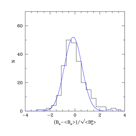
Figure 6: Histogram of the KL coefficients of the REFLEX cluster sample obtained with the reference solution (Eq. 4), and superposed unit-variance Gaussian profile shifted by $-0.14\sigma$ in order to get a better representation of the observed data. The coefficients are normalized by the eigenvalues of the REFLEX sample correlation matrix.

5 Results

Table 1 summarizes the basic results for $\Omega_{m}$ and $\sigma_{8}$ including their formal $1\sigma$ standard deviations obtained with the REFLEX cluster sample for different priors under the general assumption of a non-evolving cluster population and geometrically flat cosmologies. Typical likelihood contours are shown in Figs. 1 to 5. They illustrate the sensitivity of the analysis on important cosmological parameters. For the comparison of different KL solutions we use as reference the results obtained with $h=0.70$, $\Omega_{b}h^{2}=0.020$, $n_{\rm S}=1.0$, $\bar{z}=0.0$, $\sigma_{\rm eff}=25\,\%$, an empirical mass/X-ray luminosity relation with the parameters $A=-20.055$, $\alpha=1.652$ (denoted by M106), and the biasing model of Sheth & Tormen (1999), yielding (Fig. 4 left and the 8th row in Table 1)

$$\Omega_{m}\,=\,0.341\,^{+0.031}_{-0.028}\,,\quad\quad\sigma_{8}\,=\,0.711\,^{+0.039}_{-0.031}\,.$$ (4)

The $1\sigma$ random errors do not include cosmic variance. Compared to the results obtained by utilizing the cluster fluctuations only (Paper II), the present random errors are a factor of 2.0 smaller for $\Omega_{m}$ and a factor of 8.6 smaller for $\sigma_{8}$. This illustrates the importance of including the cluster abundance as a second criterion because it appears to be the main driver of the high accuracies reached in the present investigation. However, the results (4) are more sensitive to systematic errors compared to those solely obtained with the fluctuation analysis. Therefore, we have to evaluate the systematic errors introduced by the specific values of the priors and model assumptions in more detail.

As expected, small systematic differences ($\Delta\Omega_{m},\Delta\sigma_{8}$) are found when the Hubble constant $h$ (Freedman et al. 2001) and the spectral index of the initial scalar fluctuations $n_{\rm S}$ (see references given in Sect. 1) are changed within their respective $1\sigma$ ranges around the priors of the reference solution (see Figs. 1, 2). They are of the order of the $1\sigma$ random errors given in (4).

The systematics introduced by the $\Omega_{b}h^{2}$ ranges of, e.g., Pryke et al. (2002) appear comparatively small (see Fig. 3). A larger effect is expected when the full range $0.0095\leq\Omega_{b}h^{2}\leq 0.023$ obtained with standard Big Bang nucleosynthesis would have been used. However, the measurements of Deuterium in quasar absorption systems if primordial gives $\Omega_{b}h^{2}=0.020\pm 0.0015$, which is quite consistent with recent CMB estimates (see review of Sarkar 2002) and thus provides a good argument for the smaller confidence range adopted in the present investigation.

In order to test the stability of the results with respect to the biasing model two extreme cases are selected (see Fig. 4). The model of Sheth & Tormen (ST, 1999) although motivated by a Press-Schechter like prescription is calibrated with dark matter simulations. The pure statistical biasing model of Kaiser (KA, 1984) is mainly based on the Gaussianity of the cosmic matter field. On the large scales studied in the present investigation we do not expect large differences between the two models, as supported by the results obtained with the KL analysis (see Fig. 4 and Table 1).

Table 1. Constraints on $\Omega_{m}$ and $\sigma_{8}$ and their $1\sigma$ errors (without cosmic variance) obtained with the KL method for the REFLEX cluster sample assuming a flat space. $h$ Hubble constant. $\Omega_{b}h^{2}$: baryon density. $n_{\rm S}$ spectral index of initial scalar fluctuations. $b$ biasing model: ST Sheth & Tormen (1999); KA Kaiser (1984). $\sigma_{\rm eff}$ relative effective scatter of mass of the empirical mass/X-ray luminosity relation given in percent. $M/L$ empirical mass luminosity relation: $M/L=106$ corresponding to $A=-20.055$, $\alpha=1.652$ (obtained in RB02 with 106 clusters); $M/L=63$ corresponding to $A=-18.320$, $\alpha=1.538$ (obtained with 63 clusters). $\Omega_{m}$, $\sigma_{8}$ and their $\pm 1\sigma$ errors (no cosmic variance); $c$ concentration parameter of the NFW profile. $\Delta\Omega_{m}$ and $\Delta\sigma_{8}$: systematic differences in $\Omega_{m}$ and $\sigma_{8}$ between actual KL solution and reference solution.

$h$	$n_{\rm S}$	$\Omega_{b}h^{2}$	$b$	$\sigma_{\rm eff}$	$M/L$	$c$	$\Omega_{m}$	$+1\sigma$	$-1\sigma$	$\sigma_{8}$	$+1\sigma$	$-1\sigma$	$\Delta\Omega_{m}$	$\Delta\sigma_{8}$
$0.64$	$1.0$	$0.020$	ST	25%	106	5	$0.360$	$0.030$	$0.030$	$0.686$	$0.034$	$0.036$	$+0.019$	$-0.025$
$0.80$	$1.0$	$0.020$	ST	25%	106	5	$0.319$	$0.027$	$0.027$	$0.744$	$0.041$	$0.034$	$-0.022$	$+0.033$
$0.70$	$0.9$	$0.020$	ST	25%	106	5	$0.368$	$0.032$	$0.031$	$0.676$	$0.036$	$0.030$	$+0.027$	$-0.035$
$0.70$	$1.1$	$0.020$	ST	25%	106	5	$0.318$	$0.028$	$0.025$	$0.745$	$0.040$	$0.039$	$-0.023$	$+0.034$
$0.70$	$1.0$	$0.018$	ST	25%	106	5	$0.341$	$0.029$	$0.029$	$0.711$	$0.042$	$0.029$	$\pm 0.000$	$\pm 0.000$
$0.70$	$1.1$	$0.026$	ST	25%	106	5	$0.352$	$0.028$	$0.030$	$0.695$	$0.041$	$0.035$	$+0.011$	$-0.016$
$0.70$	$1.0$	$0.020$	KA	25%	106	5	$0.336$	$0.034$	$0.026$	$0.746$	$0.034$	$0.036$	$-0.005$	$+0.035$
$0.70$	$1.0$	$0.020$	ST	25%	106	5	$0.341$	$0.031$	$0.028$	$0.711$	$0.039$	$0.031$	$\pm 0.000$	$\pm 0.000$
$0.70$	$1.0$	$0.020$	ST	25%	63	5	$0.281$	$0.025$	$0.021$	$0.767$	$0.035$	$0.037$	$-0.060$	$+0.056$
$0.70$	$1.0$	$0.020$	ST	19%	106	5	$0.320$	$0.019$	$0.026$	$0.798$	$0.030$	$0.035$	$-0.021$	$+0.087$
$0.70$	$1.0$	$0.020$	ST	28%	106	5	$0.420$	$0.050$	$0.050$	$0.556$	$0.054$	$0.040$	$+0.079$	$-0.155$
$0.70$	$1.0$	$0.020$	ST	25%	106	4	$0.348$	$0.036$	$0.020$	$0.725$	$0.029$	$0.046$	$+0.007$	$+0.014$
$0.70$	$1.0$	$0.020$	ST	25%	106	6	$0.339$	$0.024$	$0.034$	$0.699$	$0.041$	$0.027$	$-0.002$	$-0.012$

More technically, we measured the systematics introduced by the assumption that the empirical mass/X-ray luminosity relation of RB02 is determined alternatively at the formal sample mean $\bar{z}=0.05$ and not at $\bar{z}=0.0$ yielding $\Delta\Omega_{m}=-0.004$ and $\Delta\sigma_{8}=+0.007$ (no figure). We further tested the sensitivity of the cosmological parameters on the effective scatter of the mass/X-ray luminosity relation by alternatively assuming instead of $\sigma_{\rm eff}=25\,\%$ the effective scatter of $\sigma_{\rm eff}=19\,\%$ and $28\,\%$ yielding $\Delta\Omega_{m}=-0.021$, $\Delta\sigma_{8}=+0.087$ (compare Fig. 4 left (25%) with Fig. 5 left (19%)) and $\Delta\Omega_{m}=+0.079$, $\Delta\sigma_{8}=-0.155$, respectively (no figure). We also tested the sensitivity of the cosmological parameters on the chosen mass/X-ray luminosity relation using instead of the default relation obtained with the extended RB02 sample of 106 clusters (denoted M106: $A=-20.055$, $\alpha=1.652$) a relation obtained with a strict flux-limited sample of 63 clusters (denoted M63: $A=-18.320$, $\alpha=1.538$) yielding $\Delta\Omega_{m}=-0.060$ and $\Delta\sigma_{8}=+0.056$ (compare Fig. 4 left (M106) with Fig. 5 right (M63)). Finally, we tested the effect of a value of the concentration parameter of the NFW mass density profile different from the default value $c=5$. For $c=4$ and $c=6$ we obtained $\Delta\Omega_{m}=+0.007$, $\Delta\sigma_{8}=+0.014$ and $\Delta\Omega_{m}=-0.002$, $\Delta\sigma_{8}=-0.012$, respectively (no figure).

For the correct determination of the confidence ranges caused by the combined effect of all uncertainties of the priors and model assumptions one has to analyse the complete 8-dimensional parameter space. The KL method is, however, quite computer-intensive so that the errors could only be evaluated in the following simplified manner. The approximate combined effect (conservative upper limit) is estimated by summing up the individual systematic errors. We obtain the maximum systematic errors of $\Delta\Omega_{m}=^{+0.143}_{-0.137}$ and $\Delta\sigma_{8}=^{+0.266}_{-0.243}$. A correlation of the systematics evaluated above is, however, quite unlikely. More realistic error estimates assume that the systematics are uncorrelated and that the squared $\Delta$’s can be regarded as the variances of error distributions assumed to be Gaussian. In this case the errors add quadratically and we obtain the final systematic errors

$$\sigma_{\Omega_{m}}\,=\,^{+0.087}_{-0.071}\,,\quad\quad\sigma_{\sigma_{8}}\,=\,^{+0.120}_{-0.162}\,.$$ (5)

Finally, we tested whether the Gaussianity assumed throughout the likelihood analysis is supported by the present measurements. Although the histogram of the normalized KL coefficients (Fig. 6) shows a small systematic shift of $0.14\sigma$ and some excess at large positive fluctuations relative to a zero-mean, unit-variance Gaussian profile, the latter distribution and the un-shifted observed distribution must be regarded as selected from the same parent distribution when tested on the $3\sigma$ confidence level (KS-test). The present measurements thus support the fundamental assumption of Gaussianity, although less significant compared to our first findings (see Paper II).

Figure 7: Likelihood contours obtained with the REFLEX cluster abundances only (center at $\Omega_{m}=0.32$ and $\sigma_{8}=0.71$). The comparison with Fig. 4 (left) obtained by using both cluster abundance and fluctuations shows that the KL method breaks the degeneracy between $\sigma_{8}$ and $\Omega_{m}$. Note the different scales of the diagrams.

6 Discussion and conclusions

In the present investigation cluster number counts and their spatial fluctuations are analysed for the first time simultaneously in order to constrain cosmological models. The test utilizes the complementarity of clustering and abundance of galaxy clusters and allows us to fully exploit the cosmological potential of the REFLEX survey of X-ray clusters (but see below).

For spatially flat cosmologies as suggested by all recent CMB measurements (Sect. 1) and for a non-evolving cluster population as suggested by the $z$-independent comoving REFLEX cluster number densities (Paper I), we obtain $\Omega_{m}=0.341$ for the cosmic matter density and $\sigma_{8}=0.711$ for the normalization of the matter power spectrum. The random errors range between 8-9% for $\Omega_{m}$ and 4-5% for $\sigma_{8}$, not including cosmic variance. Systematic errors can be identified and quantified so that the whole process appears to be well-controlled. Under the assumption that the systematics add quadratically the total systematic errors are found to be about 2.5 and four times larger than the random errors of $\Omega_{m}$ and $\sigma_{8}$, respectively.

Compared to the results obtained with the fluctuations only (Paper II), the combination of abundance and fluctuation measurements reduces the random errors of $\Omega_{m}$ by a factor of about two and of $\sigma_{8}$ by a factor of about nine. The main driver of the accuracy of the present results thus appears to be the cluster abundance, especially for $\sigma_{8}$ (but see below).

In contrast to many other cosmological parameter estimations we tested the assumed functional form of the sample likelihood function. As in Paper II we could verify Gaussianity on large scales – a fundamental property of the cosmic matter field. In this respect the present analysis appears to be fully consistent and self-contained.

                                                                      

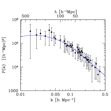
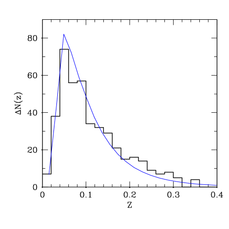
Figure 8: Comparison of the reference KL solution ($\Omega_{\rm tot}=1$, $\Omega_{m}=0.341$, $\Omega_{b}h^{2}=0.020$, $h=0.70$, $n_{\rm S}=1.0$, $\sigma_{8}=0.711$, $\sigma_{\rm eff}=25\%$, ST biasing) with REFLEX observations. Left: Power spectrum obtained with the flux-limited REFLEX sample (Paper I, points with $1\sigma$ error bars including cosmic variance) and the KL solution (continuous line). The theoretical model takes into account the effects of the different volumes covered by the present KL and the former Fourier analysis, includes the effects of the baryons, and is transformed into redshift space using the nonlinear model described in Paper I. In order to make the measured power spectrum less crowded adjacent power spectral densities and their errors were averaged. Right: Redshift histogram of the REFLEX subsample used here (steps) and the KL solution (continuous line).

The KL likelihood contours (Figs. 1 to 5) show some correlations between $\Omega_{m}$ and $\sigma_{8}$, probably indicating that the primordial part of the power spectrum is still less constrained by the REFLEX data. The correlations are, however, restricted to comparatively small $(\Omega_{m},\sigma_{8})$ ranges so that it does not make much sense to determine an $\Omega_{m}$-$\sigma_{8}$ relation from the data. Therefore, the degeneracy between $\Omega_{m}$ and $\sigma_{8}$ can be regarded as broken. The breaking of the degeneracy by the KL method using both cluster abundance and fluctuations is nicely seen when the KL reference results (Fig. 4, left) are compared with the likelihood contours obtained with the REFLEX cluster abundance only (Fig. 7).

Generally, likelihood analyses which optimize simultaneously two or more almost independent observational quantities like the power spectrum and the cluster abundance, try to find the best compromise between the individual observables and not necessarily the best fit of the different components. However, Fig.  8 shows that the best KL solution obtained with the REFLEX data is consistent with both the redshift histogram and the redshift-space power spectrum obtained with a standard Fourier method (Paper I). Note that the power spectrum was measured within a comparatively small volume to reduce correlations between different fluctuation modes. A further argument supporting the reliability of the present cosmological constraints is given by numerical fits of the amplitude of the observed power spectrum of three volume-limited REFLEX subsamples using $\Lambda$CDM models which yield $\sigma_{8}=0.70$ (Paper I). This result is at variance to the standard normalization of the $\Lambda$CDM model, but in very good agreement with the results of the present KL analysis.

The value of the cosmic matter density obtained with REFLEX is in good agreement with other recent independent measurements (see also Turner 2002). For example, Pryke et al. (2002) measured with DASI a matter density of $\Omega_{m}=0.40\pm 0.15$ for $h=0.72\pm 0.08$ and Sievers et al. (2002) measured with CBI $\Omega_{m}=0.62\pm 0.22$ (weak priors). Netterfield et al. (2002) obtained for flat geometries $\Omega_{m}=0.33\pm 0.05$, combining COBE-DMR, BOOMERANG, large-scale structure, and supernovae type Ia data. Sievers et al. (2002) found from the combination of COBE, BOOMERANG, MAXIMA-1, DASI, CBI, large-scale structure surveys, Hubble parameter determinations, and supernovae type Ia the value $\Omega_{m}=0.32\pm 0.06$. With the galaxy power spectrum of the 2dF Galaxy Redshift Survey and a new compilation of CMB data (COBE, BOOMERANG, MAXIMA-1, DASI, VSA see Scott et al. 2002, CBI see Mason et al. 2002), Percival et al. (2002) obtained for a flat cosmology $\Omega_{m}=0.313\pm 0.055$ (all $1\sigma$ errors without cosmic variance). Therefore, a significant number of independent applications appear to converge to a low matter density.

The linear theory $\sigma_{8}$ obtained with REFLEX is lower than the COBE normalization and most estimates from cluster abundance as summarized in, e.g., Table 6 in RB02. Note that values of the effective scatter $\sigma_{\rm eff}$ of the mass/X-ray luminosity relation larger than assumed here would increase this descrepancy even more. However, small $\sigma_{8}$ values were also obtained by Markevitch (1998) using a local cluster sample with ASCA X-ray temperatures and ROSAT X-ray luminosities, by Borgani et al. (2001) using the ROSAT Deep Cluster Survey, by Seljak (2001) from the empirical mass/X-ray temperature relation of nearby clusters, by Viana, Nichol & Liddle (2002) using SDSS/RASS data and the X-ray luminosity function of REFLEX clusters of galaxies, and by Bahcall et al. (2002) using clusters selected from SDSS data. In this context it is also interesting to note that the KL results are in very good agreement with the new constraints obtained by Lahav et al. (2002) from their simultaneous analysis of the amplitudes of the fluctuations probed by the 2dF Galaxy Redshift Survey and COBE, BOOMERANG, MAXIMA-1, DASI data, and with the constraints obtained with the KL analysis of the early Sloan Digital Sky Survey by Szalay et al. (2001) obtained under similar priors (as described in Lahav et al.). There is thus increasing observational evidence for a $\sigma_{8}$ value lower than previously, although some recent weak lensing results show a tendency for a higher $\sigma_{8}$ for given $\Omega_{m}$ (e.g., Hoekstra et al. 2002, van Waerbeke et al. 2002). Small $\sigma_{8}$ values help (James S. Bullock, private communication) to reduce the apparent problem of the $\Lambda$CDM model with the standard normalization to overpredict the number of low-mass satellite galaxies (Klypin et al. 1999, Moore et al. 1999).

In all the cosmological studies mentioned above including the present, various model corrections might change the final results by 10% to 30% so that more detailed analyses of possible sources of systematic errors are needed to get below this error level. Our tests for systematic errors show that the largest systematic errors are introduced by the mass/X-ray luminosity relation (as expected). In order to use the full potential of REFLEX-like cluster surveys it is thus important to have more precise measurement of this function, i.e., its shape, intrinsic scatter, redshift-dependency, etc. which are expected to be provided by detailed observations with the Chandra and XMM satellites. Future REFLEX papers will test carefully the residual effects of possible evolution of nearby clusters, the cosmological constant and related quantities (H. Böhringer et al., P. Schuecker et al., in preparation).

Regardless of these interim restrictions, the present investigation illustrates that large and fair samples of X-ray clusters of galaxies give quite clean measurements of the cosmological parameters. In addition to the abovementioned quality of $\sigma_{8}$ constraints traditionally obtained with clusters of galaxies, the $1\sigma$ random error for the matter density of $\sigma_{\Omega_{m}}=0.030$ obtained with the REFLEX data is already close to the random error of $\sigma_{\Omega_{m}}=0.010$ expected to be attainable with the CMB Planck Surveyor satellite and similar to $\sigma_{\Omega_{m}}=0.015$ attainable with the SNfactory plus SNAP supernovae satellite projects (see, e.g., Hannestad & Mörtsell 2002). Moreover, the cosmological constraints obtained with cluster data have degeneracies different from high-$z$ supernovae and CMB anisotropies (Holder, Haiman & Mohr 2001). Therefore, galaxy clusters can play a significant rôle in high precision measurements of cosmological parameters.

Appendix A Mass transformations

In this appendix we discuss mass transformations which are necessary when masses $M_{\Delta}$ are defined within radii $r_{\Delta}$ which correspond to different average density contrasts $\Delta$ and when average contrasts are related to different background densities. We are particularily interested in the relation between the masses used in the empirical mass/X-ray luminosity relation of Reiprich & Böhringer (2002) and the masses used in the theoretical mass function of Jenkins et al. (2001). To motivate the mass transformations we first assume an isothermal sphere at redshift $z=0$ and define a virial radius by

$$r_{\rm VIR}\,=\,\left[\frac{M_{\rm VIR}}{(4\pi/3)\Delta_{c}\,\rho_{c}}\right]^{1/3}\,,$$ (6)

with the average density contrast $\Delta_{c}$ which is $18\pi^{2}$ for the EdS case, and the critical EdS density $\rho_{c}=3H_{0}^{2}/8\pi G$. The virial relation then reads $G\,M_{\rm VIR}\,=\,a\,T_{\rm X}\,r_{\rm VIR}$, with $T_{\rm X}$ the temperature of the X-ray emitting gas and $a$ a structural constant. If massive clusters are simply re-scaled versions of low mass clusters (e.g., Neumann & Arnaud 2001) then $a$ is a universal constant and one obtains

$$M_{\rm VIR}\,=\,\left(\frac{a}{G}\right)^{3/2}\frac{1}{\sqrt{4\pi/3}}\,\frac{1}{\sqrt{\Delta_{c}}}\frac{1}{\sqrt{\rho_{c}}}\,\,T_{\rm X}^{3/2}\,.$$ (7)

The assumption of an isothermal sphere mass distribution thus yields for a given redshift and temperature the mass-density contrast relation $M_{\rm VIR}/M_{\Delta}=(\Delta/\Delta_{c})^{0.5}$. Deviations from isothermality changes this relation as can be seen in Horner et al. (1999) who found from spatially resolved temperature measurements the empirical relation $M_{\rm VIR}/M_{\Delta}=(\Delta/\Delta_{c})^{0.266}$, consistent with the mass density profile $\rho(r)\sim r^{-2.4}$. In order to be consistent with our reference to high-quality dark matter simulations we assume a Navarro, Frenk & White (NFW, 1997) profile. In this case we have to deal with a mass ratio $M_{\rm VIR}/M_{\Delta}\equiv\Pi(\Delta_{c},\Delta)$ which can only be obtained numerically using

$$\frac{M_{\Delta_{1}}}{M_{\Delta_{2}}}\,=\,\frac{\Delta_{1}}{\Delta_{2}}\,\cdot\,\left(\frac{r_{\Delta_{1}}}{r_{\Delta_{2}}}\right)^{3}\,,$$ (8)

$$\frac{M_{\Delta_{1}}}{M_{\Delta_{2}}}\,=\,\frac{\ln\left(1+c\,r_{\Delta_{1}}/r_{200}\right)\,-\,\frac{cr_{\Delta_{1}}/r_{200}}{1+c\,r_{\Delta_{1}}/r_{200}}}{\ln\left(1+c\,r_{\Delta_{2}}/r_{200}\right)\,-\,\frac{cr_{\Delta_{2}}/r_{200}}{1+c\,r_{\Delta_{2}}/r_{200}}}\,,$$ (9)

where $c$ is the concentration parameter which we assume to be independent of mass and redshift. Iterative solution for $r_{\Delta_{1}}/r_{\Delta_{2}}$ yields the mass ratio $\Pi$ where the normalization radius $r_{200}$ of the NFW profile cancels out. Due to its definition via a mass ratio, $\Pi$ has the property $\Pi(\Delta_{1},\Delta_{2})\cdot\Pi(\Delta_{2},\Delta_{3})=\Pi(\Delta_{1},\Delta_{3})$, yielding

$$\frac{M_{\rm VIR}(0)}{M_{200}^{\rm EdS}(0)}\,=\,\Pi\left(\Delta_{c}(0),\Delta_{c}^{\rm EdS}(0)=18\pi^{2}\right)\,.$$ (10)

The arguments indicate that the quantities are determined at redshift $z=0$. Note that the density contrast $\Delta_{c}^{\rm EdS}(0)$ approximately defines the same mass $M_{200}^{\rm EdS}$ as used in the empirical mass-luminosity relation of Reiprich & Böhringer.

With the function $E(z)$ defined in Sect. 3, a possible redshift-dependence might be introduced by $\rho_{c}(z)\sim E^{2}(z)$ and $\Delta_{c}(z)=18\pi^{2}+82\left[\Omega_{m}(z)-1\right]-39\left[\Omega_{m}(z)-1\right]^{2}$ with $\Omega_{m}(z)=\Omega_{m}(1+z)^{3}/E^{2}(z)$ for spatially flat geometries (Bryan & Norman 1998). For a given temperature we thus obtain

$$M_{\rm VIR}(z)\,=\,M_{\rm VIR}(0)\,\,\frac{\Pi\left(\Delta_{c}(z),\Delta_{c}(0)\right)}{E(z)}\,,$$ (11)

so that the relation between a virialized mass at redshift $z$ and the mass as defined in the empirical mass/X-ray luminosity relation becomes

$$M_{\rm VIR}(z)\,=\,M_{200}^{\rm EdS}(0)\,\cdot\,\Pi\left(\Delta_{c}(z),\Delta_{c}^{\rm EdS}(0)\right)\,\cdot\,\frac{1}{E(z)}\,.$$ (12)

Finally, we have to relate $M_{\rm VIR}(z)$ to the mass as defined in the universal mass function of Jenkins et al. (2001). Here, the masses are defined by the radius of the spherical overdensity of $18\pi^{2}$ with respect to the $\Omega_{m}$-dependent background density. Denoting this mass by $M_{\rm SO(180)}(z)$ we have

$$M_{\rm SO(180)}(z)\,=\,M_{\rm VIR}(z)\,\,\Omega_{m}(z)\,\,\tilde{r}^{3}\,,$$ (13)

where $\tilde{r}=r_{\rm SO(180)}/r_{\rm VIR}$ is obtained iteratively from the NFW mass density profile using

$$\ln(1+c\tilde{r})-1+\frac{1}{1+c\tilde{r}}=\Omega_{m}(z)\left[\ln(1+c)-\frac{c}{1+c}\right]\,.$$ (14)

In the main text a non-evolving cluster population is assumed so that the relevant equations are evaluated either at $z=0.0$ or alternatively at $z=0.05$.