Photometry Results for the Globular Clusters M10 and M12: Extinction Maps, Color-Magnitude Diagrams, and Variable Star Candidates

Abstract

We report on photometry results of the equatorial globular clusters (GCs) M10 and M12. These two clusters are part of our sample of GCs which we are probing for the existence of photometrically varying eclipsing binary stars. During the search for binaries in M10 and M12, we discovered the signature of differential reddening across the fields of the clusters. The effect is stronger for M10 than for M12. Using our previously described dereddening technique, we create differential extinction maps for the clusters which dramatically improve the appearance of the color-magnitude diagrams (CMDs). Comparison of our maps with the dust emissivity maps of Schlegel, Finkbeiner, & Davis (SFD) shows good agreement in terms of spatial extinction features. Several methods of adding an $E_{V-I}$ zero point to our differential maps are presented of which isochrone fitting proved to be the most successful. Our $E_{V-I}$ values fall within the range of widely varying literature values. More specifically, our reddening zero point estimate for M12 agrees well with the SFD estimate, whereas the one for M10 falls below the SFD value. Our search for variable stars in the clusters produced a total of five variables: three in M10 and two in M12. The M10 variables include a binary system of the W Ursa Majoris (W UMa) type, a background RR Lyrae star, and an SX Phoenicis pulsator, none of which is physically associated with M10. M12’s variables are two W UMa binaries, one of which is most likely a member of the cluster. We present the phased photometry lightcurves for the variable stars, estimate their distances, and show their locations in the fields and the CMDs of the GCs.

1 Introduction

Variable stars have historically served as important tools and “laboratories” in our understanding of star formation, the formation of stellar clusters, and the calibration of distance determination methods. In particular, the study of eclipsing binary stars (EBs) in a globular clusters (GC) may be used to obtain a value for the cluster’s distance and a constraint concerning turnoff masses of the GC stars (Paczyński, 1996).

Simply detecting EBs in the fields of GCs and confirming cluster membership is a straightforward - though data-intensive - task. These systems expand the relatively meager sample of EBs which are currently confirmed GC members (see for example Mateo, 1996; McVean et al., 1997; Rubenstein, 1997; Rucinski, 2000; Clement et al., 2001, and references therein). A statistical evaluation of the number of known member EBs in GCs can help in the determination of physical quantities such as the binary frequency in GCs as a parameter in the study of dynamical evolution of GCs (Hut et al., 1992).

Member stars of the clusters interact with each other, primarily toward the core of the GC where the stellar density is much higher than in the GC halo. Due to consequent redistribution of stellar kinetic energies and orbits, the core stars gradually diffuse into the halo which, as a result, grows in size. At the same time, the cluster core itself shrinks, and its density will theoretically reach infinitely high values in a finite period of time (10-20 $t_{relax}$, according to simulations, see Binney & Tremaine, 1987), a phenomenon known as core collapse. Binary stars will most likely be located toward the GC center due to the fact that a) they are more likely to form in regions of high stellar density, and b) they will sink toward the core due to their high masses after a few cluster relaxation times. Since the binding energy of one individual hard binary can be as high as a few to ten percent of the binding energy of the entire GC, they may act as an energy source (similar to the nuclear reaction inside the centers of stars) to halt core collapse. A binary fraction as low as 10% in the cluster core will suffice to cool the the central region of the GC by reversing the outward flow of energy toward the halo (Binney & Tremaine, 1987; Hut et al., 1992) and arrest core collapse.

An additional use of simply detecting member-EBs in GC lies in the calibration of absolute magnitudes of and corresponding distances to W Ursa Majoris (W UMa) binaries (Rucinski, 1994, 1995, 2000, see also Section 4.3).

The simultaneous analysis of photometric and spectroscopic data for individual EB systems can moreover provide a direct estimate of the distance to the system (Andersen, 1991; Paczyński, 1996), and thus, if the EB is a GC member, to the GC itself. The main sources of error in this distance determination are a) the relation between surface brightness and effective temperature of the binary and b) the precise determination of the interstellar reddening along the line of sight to the EB which can vary substantially across the field of view of the GC. The distance determination method itself, however, is free of intermediate calibration steps and can provide direct distances out to tens of kpc. In turn, the knowledge of the distances to GCs can then be used to calibrate a variety of other methods, such as the relation between luminosity and metallicity for RR Lyrae stars. The very same analysis can, in principle, be used to obtain the Population II masses of the individual components of the EB system (Paczyński, 1996) to provide a fundamental check of stellar models at low metallicities.

We are currently undertaking a survey of approximately 10 Galactic GCs with the aim of identifying photometrically variable EBs around or below the main-sequence turnoff (MSTO). Our observing strategy, aimed at detecting binaries in the period range of approximately 0.1 to 5 days (Hut et al., 1992) consists of repeated observations of a set of GCs during each night of an observing run. Multiple runs are helpful in detecting variables with a period of close to one day (or to a multiple thereof).

M10 (NGC 6254) and M12 (NGC 6218) are two equatorial clusters in our sample, located at $\alpha_{2000}=16^{h}57^{m}08.9^{s}$ and $\delta_{2000}=-4^{\circ}05^{{}^{\prime}}58^{{}^{\prime\prime}}$ ($l=15.14^{\circ}$ ; $b=23.08^{\circ}$), and at $\alpha_{2000}=16^{h}47^{m}14.5^{s}$ and $\delta_{2000}=-1^{\circ}56^{{}^{\prime}}52^{{}^{\prime\prime}}$ ($l=15.72^{\circ}$ ; $b=26.31^{\circ}$), respectively (Harris, 1996). They are nearby (M10: 4.4 kpc and M12: 4.9 kpc) which makes them attractive targets for monitoring studies. Both clusters have been probed for the existence of variable stars in the past (for a summary, see Clement et al., 2001). Previous studies searched for luminous variables on the red giant and/or horizontal branch of the clusters and therefore do not overlap with the magnitude range covered in this work.

Details on our photometry observations and basic data reductions are given in Section 2. We discuss how we correct for interstellar extinction along the line of sight to M10 and M12 in Section 3. Section 4 contains the description and the results of our search for variable stars in the clusters including the phased lightcurves for the variables in the cluster fields and our estimates concerning distances and cluster membership. The methods used for Sections 3 and 4 are outlined in detail in two previous publications, namely von Braun & Mateo (2001, BM01 hereafter) and von Braun & Mateo (2002, BM02 hereafter) , respectively. Finally, we summarize and conclude with Section 5.

2 Observations and Data Reductions

2.1 Observations

The observations for M10 and M12 were obtained during multiple runs between June 1995 and May 1999 at the Michigan-Dartmouth-MIT (MDM) Observatory’s 1.3m and the Las Campanas Observatory (LCO) 1m Swope Telescope. Tables 1 and 2 list the details. During all observing runs, we used $2048^{2}$ pix CCDs with different field sizes and standard Johnson-Cousins $VI$ filters. The number of epochs was about evenly divided between $V$ and $I$. During two runs, we took additional shorter (10s) exposures to complete the CMDs in the brighter regions (see Tables 1 & 2). These shorter observations were not used to look for variable stars because of infrequent time coverage. All exposures are centered on the cluster center itself. The reason for the rather large number of observing runs with relatively few epochs per run (compared to the other clusters in our sample) is the equatorial location of both M10 and M12. Consequently, neither cluster is ever located closer to the zenith than $30^{\circ}$ from MDM as well as from LCO. As a result, the clusters were observed for only up to $\sim$ 2 hours each per night when seeing conditions were good, with the rest of the time dedicated to other clusters in our sample.

2.2 Data Processing and Reduction

The details of the IRAF processing as well as the basic data reduction of the May 1998 data are described in BM01, section 2.1. The IRAF processing of the other data sets was performed in the same manner. All data were reduced using DoPHOT (Schechter, Mateo, & Saha, 1993) in fixed-position mode after aligning every image to a deep-photometry template image consisting of the best seeing frames for each filter from every run (see BM01). Aperture corrections and a variable PSF were fitted to the May 1998 data as second order polynomials in $x$ and $y$. Our astrometric solutions for both cluster fields, based on approximately 120 US Naval Observatory (USNO) reference stars (Monet et al., 1996), respectively, produced linear fits in $x$ and $y$ with a random mean scatter (rms) of around 0.2 arcsec, consistent with the USNO precision. Photometric calibration of the May 1998 data is described in BM01.

All other data were shifted to the coordinates and the photometric system of the May 1998 600s exposures, including the shorter exposures. In the process of combining the 10s exposures with the deep data, we fit for a zero point and color term to match the two sets, thereby effectively treating the deep data as photometric standards. Whenever we had two measurements for the same star, we kept the one with the lower photometric error associated with it (in most cases, this was the 600s measurement). The division between the two photometry sets occurs around $V\sim 17-17.5$. We note that we are sensitive to variable detection to a magnitude as bright as $V\sim 16.5$ since the CCDs we used have different quantum efficiencies and some of the observations were taken through thin layers of clouds.

Photometric results for every star, weighted by the inverse square of the DoPHOT photometric error for the respective measurement, were averaged with the only requirement that a star appear in approximately 20% or more of the epochs. This condition is much less stringent than its corresponding counterpart in the analysis of NGC 3201 (see BM01 and BM02) where we set this threshold to 75%. The reason for the difference lies in the varying field sizes of the CCDs used for M10 and M12 (see Tables 1 & 2). A larger field (LCO data) will obviously include more stars than a smaller one, whereas a higher spatial resolution (MDM data) allows us to get closer to the GC center with our reductions.

2.3 Photometry Results and Comparison to Previous Studies

Our photometry results are presented, in the form of CMDs, in Figures 1 (M10) and 2 (M12). Based on similarities between the undereddened CMDs of NGC 3201 (presented in BM01) and M10 it appears that M10 suffers from differential reddening across the field of view, as previously suggested by, e.g, Kennedy, Bates, & Kemp (1996). M10’s main sequence is broad, especially around the MSTO where the reddening vector (Cardelli, Clayton, & Mathis, 1989; Schlegel, Finkbeiner, & Davis, 1998) is approximately perpendicular to a hypothetical isochrone fit to this particular region. Its subgiant branch, giant branch, and horizontal branch (HB) display the same feature, whereas the fainter region of the main sequence ($V>20$), where the reddening vector is almost parallel an isochrone fit to the region, appears tighter. This behavior clearly rules out any sort of photometric error as the reason for the broadness of the CMD features since, in that case, one would observe well defined MSTO and subgiant branch regions and a main sequence which would flare up at fainter magnitudes. M12’s CMD, does not display the signature of differential extinction as strongly as M10, indicating that the effects of differential reddening across its field are small, despite the fact that the two clusters are separated by less than $3^{\circ}$ in the sky.

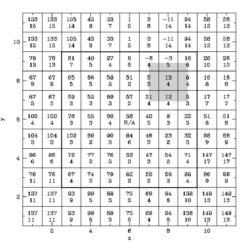
Figure 5: M10 – Differential $E_{V-I}$ values (top number) with associated errors (bottom number) relative to the average $E_{V-I}$ of the fiducial region (shown in grey for reference). Each pixel is about 140 arcsec on the side. The size and orientation of the field is the same as in Figure 3. The pixel in the map with an error value listed as N/A did not contain enough stars for a fit, due to saturation and crowding in the cluster center. Its $E_{V-I}$ was obtained by interpolation from neighboring pixels. The average reddening with respect to the fiducial region is $E_{V-I}=68\pm 41$ mmag for the entire field and $E_{V-I}=49\pm 28$ mmag for the inner part, shown in the image. The subregions in this inner part carry higher significance due to the higher number of cluster stars they contain. To obtain a map of absolute $E_{V-I}$ values, a reddening zero point has to be added to the pixel values. We discuss this zero point in Section 3.2. Finally, in order to get absolute values for $E_{B-V}$, one needs to multiply the absolute $E_{V-I}$ value (i.e., including zero point) by 0.7273 (Schlegel, Finkbeiner, & Davis, 1998).

In our photometry we estimate the MSTO of M10 to be around $V-I_{MSTO}\sim 0.88$ & $V_{MSTO}\sim 18.5$ (Figure 1), and the one of M12 to be at $V-I_{MSTO}\sim 0.84$ & $V_{MSTO}\sim 18.35$ (Figure 2). Two recent $VI$ studies present themselves as a means for photometry comparison: the extensive $VI$ GC-CMD catalog of Rosenberg et al. (2000, RB00 hereafter) and the Hubble Space Telescope (HST) study of M10, M22, and M55 of Piotto & Zoccali (1999, PZ99 hereafter). For M12 we find excellent agreement with RB00 for our photometry for both $(V-I)_{MSTO}$ and $V_{MSTO}$. For M10 our MSTO is slightly bluer and brighter than that of RB00 ($(V-I)_{MSTO}\sim 0.92$ & $V_{MSTO}\sim 18.6$). We attribute this to the fact that the region of M10 observed by RB00 lies to the East of the cluster center where we find higher differential extinction compared to the rest of the cluster field (see Section 3.1, and Figs. 3 and 5). Plotting our data which fall into the R00 field results in a location of the MSTO within 0.02 mags of the R00 MSTO which approaches the limits of the rms of the photometry.

The agreement between our M10 results and the HST photometry of PZ99, however, is not as good since their MSTO is at $(V-I)_{MSTO}>1$. As one can see in Figure 1, the range in our data does not extend to values redder than $(V-I)_{MSTO}\sim 0.95$. Since a direct star-by-star comparison between our data and PZ99 is not possible, we cannot give a good explanation for this discrepancy. One possible reason, however, might be a zero point drift in the HST photometry which has been noticed in studies such as Gallart et al. (1999), especially since PZ99’s photometry zero point is based on HST data.

In addition, we compared our MSTO magnitude to two $BV$ studies of M10 (Hurley, Richer, & Fahlman, 1989) and M12 (Sato, Richer, & Fahlman, 1989). The $V_{MSTO}$ for both M10 and M12 is estimated to be at 18.4, in good agreement with our results.

3 Dereddening

3.1 Differential Extinction

As mentioned above, the calibrated CMDs in Figures 1 and 2 show the effects of differential reddening across the respective field of view. In order to get precise magnitudes and intrinsic colors for potential GC-member binaries in the clusters, we created differential extinction maps for M10 and M12 from our data for these clusters. The method we used is outlined in detail in BM01, section 2.2 and figures 1-4. We will briefly review the most important steps here and outline the difference between the method used for NGC 3201 (BM01) and the one used here.

For each cluster, we chose a fiducial region in which little differential reddening occurred, whose overall extinction is low compared to the rest of the field, and which contained a sufficient number of stars to fit a polynomial to the main sequence for stars with $18.5<V<21$ and $0.7<V-I<1.4$. The field of view of each cluster was then divided into subregions of different sizes such that the number of stars in each of the subregions was large enough to produce a statistically significant result. For each of the subregions, an average offset between its stars and the polynomial fit along the reddening vector with slope 2.411 (Schlegel, Finkbeiner, & Davis, 1998, table 6, column 4 for Landolt filters) was calculated after $1\sigma$-outliers were deleted with an iteration. This calculated average offset corresponds to the differential $E_{V-I}$ of each star in the subregion with respect to the fiducial region, i.e., how much more extinction the stars in the subregions suffer than the ones in the fiducial region.

The slope of the reddening vector for the analysis of NGC 3201 in BM01 was 1.919, calculated using table 3 in Cardelli, Clayton, & Mathis (1989). The central wavelength of the $I$ filter in Cardelli, Clayton, & Mathis (1989) is around 9000 Å, whereas the filter used during the May 1998 LCO observing run has a $\lambda_{central}\sim 8100$ Å, closer to the value given in table 6 of Schlegel, Finkbeiner, & Davis (1998) for Landolt filters. As a result, the conversion between $E_{B-V}$ to $E_{V-I}$ changes to $E_{V-I}=1.375\times E_{B-V}$, and the slope of the reddening vector changes to $A_{V}/E_{V-I}=2.411$. We comment on the implications of this change in Section 3.2.4.

We present our results for M10 and M12 in the form of differential extinction maps in Figures 3 (M10) and 4 (M12). North is up and East is to the left (see coordinate grid on the figure included for reference). Dark corresponds to regions of higher extinction relative to the fiducial region. For reference we show the approximate locations of the cluster center and core radii (from Harris, 1996) as well as the fiducial regions of the clusters. The sizes of the pixels in these maps vary with stellar density from $\sim$ 140 arcsec on the side towards the center of the field to $\sim$ 280 arcsec on the side in the outer regions of the CCD. Compared to our analysis of NGC 3201 (BM01) the resolution of these extinction maps is lower by a factor of four (in area) due to the lower cluster-star density in these pixels.

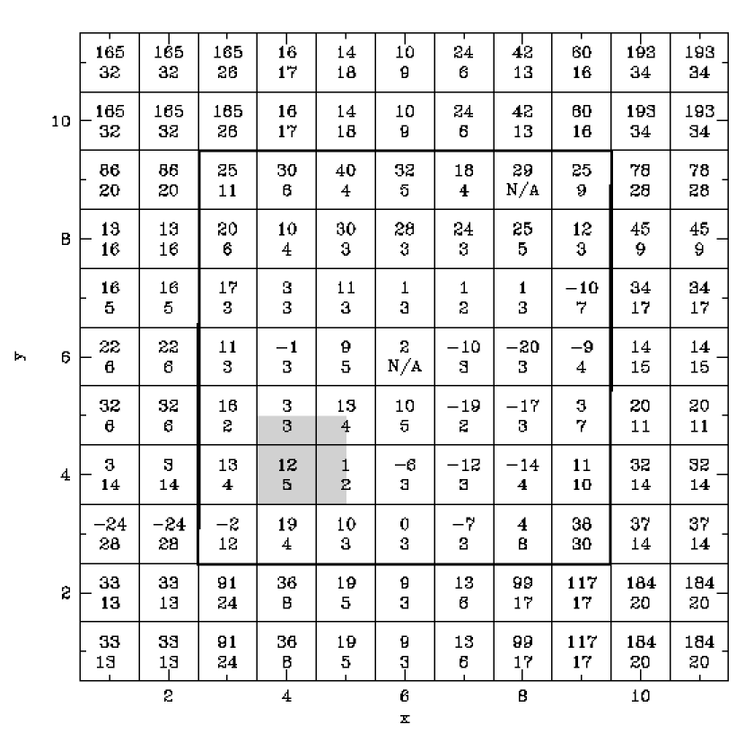
Figure 6: M12 – Differential $E_{V-I}$ values (top number) with associated errors (bottom number) relative to the average $E_{V-I}$ of the fiducial region (shown in grey for reference). Each pixel is about 140 arcsec on the side. The size and orientation of the field is the same as in Figure 4. The pixels in the map with error values listed as N/A did not contain enough stars for a fit. Their $E_{V-I}$ were obtained by interpolation from neighboring pixels. The average reddening with respect to the fiducial region is $E_{V-I}=40\pm 58$ mmag for the entire field and $E_{V-I}=9\pm 15$ mmag for the inner part (shown) of the field where the errors are smaller. To obtain a map of absolute $E_{V-I}$ values, a reddening zero point has to be added to the pixel values. We discuss this zero point in Section 3.2. Finally, in order to get absolute values for $E_{B-V}$, one needs to multiply the absolute $E_{V-I}$ value (i.e., including zero point) by 0.7273 (Schlegel, Finkbeiner, & Davis, 1998).

The average $E_{V-I}$ relative to the fiducial region (field minus fiducial) is $68\pm 41$ mmag for M10 and 40 $\pm$ 57 mmag for M12; the errors represent the standard deviation about the mean (BM01). The individual subregions’ average $E_{V-I}$ values in millimagnitudes relative to the fiducial region are shown as the top number in each of the pixels in the grids of Figures 5 and 6. The bottom number in each of the pixels corresponds to our estimate for the error in the mean for the corresponding $E_{V-I}$ value (see BM01, section 2.2, item 7 for a description of our error analysis). The location of the fiducial region is shown in grey in each of the two Figures. We further show the division between an outer “ring” of subregions and the inner part of the field. The inner subregions in each of the fields typically contain higher numbers of stars and have lower errors associated with them. The stellar density is especially low towards the corners of the fields. The average $E_{V-I}$ for only the inner part of the field compared to the fiducial region is $49\pm 28$ mmag for M10 and $9\pm 15$ mmag for M12.

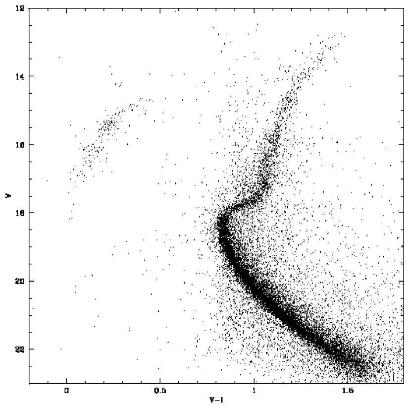
Figure 7: The internally dereddened CMD of M10. $V$ and $V-I$ indicate the location of the data points after the differential reddening with respect to the fiducial region was corrected for, i.e., after the inverse values of Fig. 5 were applied to the data. No reddening zero point is applied to the data in this plot. The improvement of the appearance of the CMD over Figure 1 is immediately obvious. The flaring of the data at $V\sim 17$ is most likely due to the low signal-to-noise of the 10s exposures at these magnitudes.

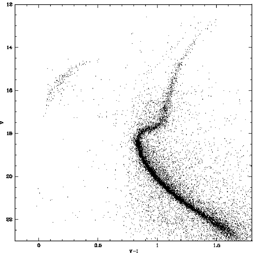
Figure 8: The internally dereddened CMD of M12. $V$ and $V-I$ indicate the location of the data points after the differential reddening with respect to the fiducial region was corrected for, i.e., after the inverse values of Fig. 6 were applied to the data. No reddening zero point is applied to the data in this plot. Note the improvement of the appearance of the CMD over Figure 2. The flaring of the data at $V\sim 17$ is most likely due to the low signal-to-noise of the 10s exposures at these magnitudes.

To illustrate the effects of our internal dereddening method, we show, in Figures 7 and 8, the CMDs after applying the extinction maps (differential reddening correction) to the data. The data points are now all shifted to the CMD-location of the stars in the respective fiducial region, that is, no absolute reddening zero point has been applied. The improvement is clearly visible in both cases and especially obvious for M10 (compare with Figures 1 and 2). The width of the main sequence of Fig. 7 has, by applying the differential reddening map, decreased to a fraction of its former value in Fig. 1. The subgiant, giant, and horizontal branches have become much more defined. Even M12’s main sequence is significantly tighter in Figure 8, and the scatter of the stars about its subgiant and horizontal branches is much lower than in Figure 2. In both differentially dereddened CMDs the small flaring of the data points at the faint end of the giant branch is most likely due to the low signal-to-noise of the 10s exposures at these magnitudes.

3.2 Reddening Zero Point Determination

At this point, our extinction values for M10 and M12 are differential, that is, they show $E_{V-I}$ with respect to a fiducial region in the respective cluster field. This fiducial region itself suffers some mean interstellar extinction. In order to a) make our reddening maps a useful tool, and b) determine intrinsic magnitudes and colors for binary system GC-member candidates, we need to determine this reddening zero point to add to our differential $E_{V-I}$ values. As described in BM01, this cannot be done using our data alone. We therefore use results from previous studies, as described below. We note that a direct comparison with literature values should be taken with caution since usually only a single numerical value for an average $E_{V-I}$ per cluster is given whereas our result is a map of extinction across the field of the cluster.

3.2.1 Using Basic Isochrone Fitting

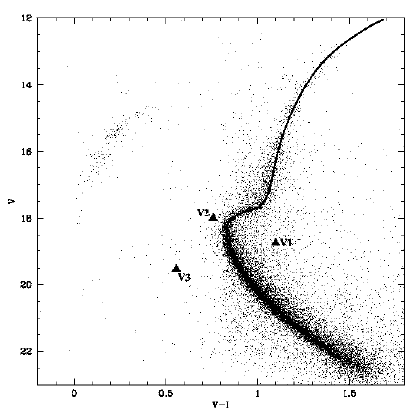
Figure 9: Differentially dereddened CMD of M10 with overlain VDB best-fit isochrone and locations of variable stars. For this fit: [Fe/H] = –1.54, age = 16 Gyrs, d = 5.1 kpc, and the $E_{V-I}$ zero point, to which any differential extinction has to be added, is 0.23. All CMD features are well traced out by the VDB isochrone. The 16 Gyr isochrone produced the better fit than the 18 Gyr one, but from the appearance of the CMD, it seems that perhaps a 17 Gyr VDB isochrone, if it were available, would produce an even better fit than the one shown here. We also show in this Figure the locations of the variable star candidates in the CMD of M10. The data presented, including the variable stars, are dereddened to the M10 fiducial region. No reddening zero point is applied. The variables are plotted at maximum brightness. From this figure alone, it seems that none of the variables we found in the field of M10 are members of the cluster. It should be noted that since we only use our 600s data for binary detection, we are not sensitive to variables brighter than $V\sim 16.5$.

The most straightforward method of determining the extinction zero point is fitting isochrones to our differentially dereddened data (as performed in BM01) . Thus, the obtained $E_{V-I}$ corresponds to the reddening zero point to add to the differential $E_{V-I}$-values (see BM01, section 4.2.1). We performed basic isochrone fitting using a set of isochrones provided by Don VandenBerg (D. VandenBerg 2000, private communication, based on evolutionary models by VandenBerg et al., 2000, hereafter VDB). Simultaneously fitting age, distance, and extinction produced the fits shown in Figures 9 (M10) and 10 (M12). For an estimate of [Fe/H], we used isochrones with values of [Fe/H] ranging from –1.14 to –2.31, straddling the cluster [Fe/H] values in Harris (1996) of –1.52 for M10 and –1.48 for M12.

M10

The isochrone fit for M10, shown in Figure 9, was obtained using the following parameters: [Fe/H] = –1.54, age = 16 Gyrs, d = 5.1 kpc ($V_{0}-M_{V}=13.55$), and the $E_{V-I}$ zero point, to which any differential extinction has to be added, is 230 mmag. All shapes of the CMD features are well traced out by the VDB isochrone. The 16 Gyr isochrone produced a slightly better fit than the 18 Gyr one, but from the appearance of the CMD, it seems that perhaps a 17 Gyr VDB isochrone, if it were available, would produce an even better fit than the one shown here. The value for [Fe/H] is similar to the Harris (1996) one of –1.52, whereas our distance estimate of 5.1 kpc is slightly higher than the Harris (1996) one of 4.4 kpc.

M12

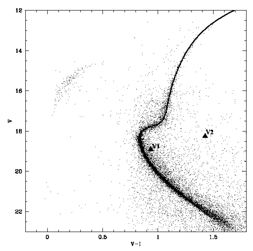
Figure 10: Differentially dereddened CMD of M12 with overlain VDB best-fit isochrone and locations of variable stars. For this fit: [Fe/H] = –1.54, age = 16 Gyrs, d = 4.9 kpc, and the $E_{V-I}$ zero point is 0.24. All features of the CMD, including the subgiant branch and the RGB, are very well traced out. The only minor deviation between the loci of the data points and the isochrone fit occurs at $V\sim 21.5$. The above isochrone parameters agree with the values for M12 in Harris (1996) and the SFD $E_{V-I}$ estimates for this region. Also shown are the locations of the variable star candidates in the CMD of M12. The data presented, including the variable stars, are dereddened to the M12 fiducial region. No reddening zero point is applied. The variables are plotted at maximum brightness. From this figure alone, it seems that the variable V1 is a cluster member whereas V2 is not. It should be noted that since we only use our 600s data for binary detection, we are not sensitive to variables brighter than $V\sim 16.5$.

Since M12’s undereddened CMD is very similar to the one of M10, apart from the much lower differential reddening, it is no surprise that the parameters for the VDB isochrone fit shown in Figure 10 are almost identical to the ones used for M10: [Fe/H] = –1.54, age = 16 Gyrs, d = 4.9 kpc ($V_{0}-M_{V}=13.46$), and the $E_{V-I}$ zero point is 240 mmag. Again all features of the CMD, including the subgiant branch and the RGB, are very well traced out. The only minor deviation between the loci of the data points and the isochrone fit occurs at $V\sim 21.5$. The above isochrone parameters agree with the values for M12 in Harris (1996).

3.2.2 Using SFD Maps

A second option in the determination of the reddening zero point is to simply calculate the average offset between our maps and the SFD dust maps. If the two maps trace out similar dust features, the offset between the maps should approximately be constant everywhere in the field. This average offset then corresponds to the estimate of the reddening zero point based on the comparison between our extinction maps and the SFD maps (based on dust emissivity).

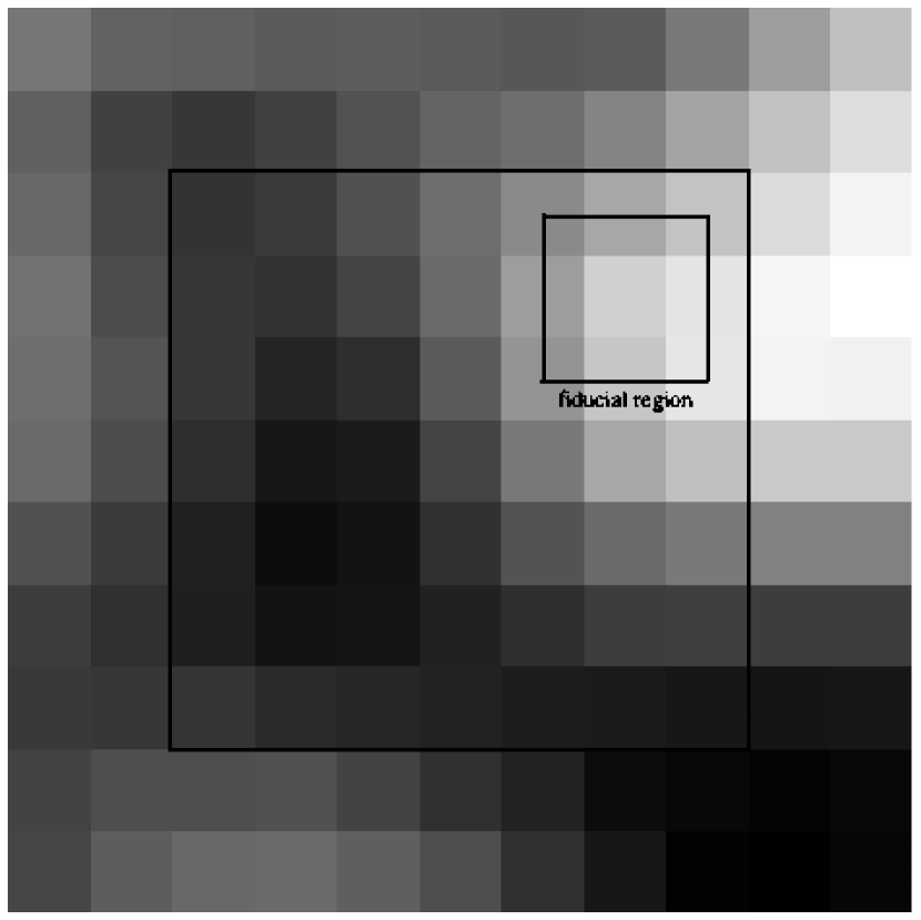
Figure 11: Graphical Representation of the SFD Map in the region of M10. The location of the fiducial region is given for reference. Orientation, size, and pixel sizes are the same as in Figures 3 and 5. Darker regions correspond to higher extinction. The extinction ranges from $E_{V-I}=344$ to 411 mmag. The average reddening is $E_{V-I}=387\pm 17$ mmag for the entire field and $E_{V-I}=389\pm 16$ mmag for the inner part of the field.

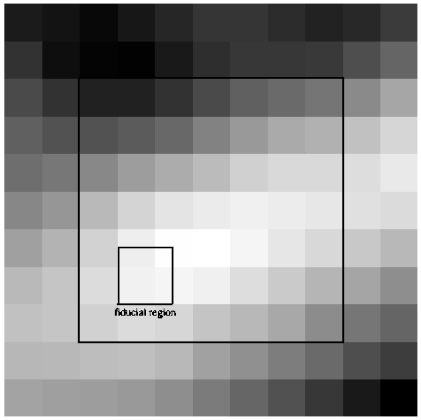
Figure 12: Graphical Representation of the SFD Map in the region of M12. The location of the fiducial region is given for reference. Orientation, size, and pixel sizes are the same as in Figures 4 and 6. Darker regions correspond to higher extinction. The extinction ranges from $E_{V-I}=241$ to 271 mmag. The average reddening is $E_{V-I}=254\pm 8$ mmag for the entire field and $E_{V-I}=250\pm 7$ mmag for the inner part of the field.

We show the pixel-interpolated SFD maps of our fields of view of M10 and M12 in Figures 11 and 12. The orientation and field sizes of Figures 11 and 12 are identical to the ones in Figures 3 and 4, respectively. As before, darker regions correspond to regions of higher extinction. We added the location of the fiducial region for reference in each Figure. For M10, the average reddening of the SFD map is $E_{V-I}=387\pm 17$ mmag for the whole field and $389\pm 16$ mmag for the inner region (see Figure 5). The errors represent the standard deviation about the mean. For M12, these values are $E_{V-I}=254\pm 8$ mmag for the whole field and $250\pm 7$ mmag for the inner region. Note that these numbers are estimates for the full extinction along the line of sight, i.e., they contain a reddening zero point. The SFD estimates agree well with Harris (1996) who quotes $E_{V-I}=382$ mmag for M10 and $E_{V-I}=258$ mmag for M12.

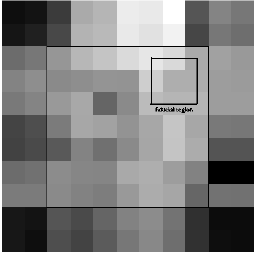
Figure 13: Graphical Representation of the difference between our extinction map for M10 (Fig. 3) and the SFD Map of the same region (Fig. 11). The location of the fiducial region is given for reference; the orientation, size, and pixel sizes are the same as in Figures 3 and 5. Darker regions correspond to areas where our maps indicate more differential extinction (relative to the fiducial region) than the SFD map. It is obvious that the especially the inner region is featureless, indicating good spatial agreement between the two maps. The pixels toward the edges of the map contain fewer cluster stars causing any calculated differential reddening to have a higher associated rms error which results in the “noisy” appearance of the ring around the inner region. The average reddening of the whole field is $E_{V-I}=319\pm 35$ mmag and $E_{V-I}=340\pm 16$ mmag for the inner region.

As a first step in the calculation of the average offset between the two independent reddening estimates, we subtracted our extinction maps from the SFD maps of the corresponding regions. The resulting images are shown in Figures 13 (M10) and 14 (M12). As in BM01, figure 7, darker regions correspond to areas where our maps indicate more differential extinction (relative to the fiducial region) than the corresponding SFD map. We show the locations of the fiducial regions as well as the border between inner and outer regions (see above) for reference.

M10

The difference map for M10 (Figure 13) indicates that our extinction map and the SFD map for M10 spatially agree quite well, particularly in the inner region of the image which basically shows no residual features at all. The determination of the differential extinction towards the edges of the map is less precise due to the lower number of cluster stars in these regions (see Figure 5) and thus appears more noisy. The average reddening of the whole field of Figure 13 (the difference map) is $E_{V-I}=319\pm 35$ mmag, whereas for only its inner region, it is $E_{V-I}=340\pm 16$ mmag. It is worth noting that for the inner region, the rms of this difference map of 16 mmag is smaller than the rms of our extinction map (28 mmag; see Figure 3) and equal to the rms the SFD map for M10 (16 mmag; see Figure 11), indicating that the features traced out by both maps are correlated.

The value 340 mmag corresponds to our estimate for the reddening zero point as determined by using the SFD maps. We were simply unable, however, to produce an isochrone that resulted in a fit to our data using this estimate of $E_{V-I}$, even when widely varying the values for distance, age, and [Fe/H] (see Section 3.2.3 for discussion). We therefore adopt our estimate of 230 mmag, as determined by the VDB isochrones, as the reddening zero point for M10 (see previous Subsection).

M12

Similar to M10, the two maps for M12 (Figures 4 and 12) agree well, resulting in a difference image (Figure 14) which is featureless except in the regions towards the corner of the image. The average reddening of the entire difference map (Figure 14) is $E_{V-I}=214\pm 53$ mmag, whereas for only its inner region, it is $E_{V-I}=241\pm 11$ mmag. The value 11 mmag as the rms is comparable to the rms of the SFD map (7 mmag; see Figure 12) and lower than the rms for our extinction map (15 mmag; see Figure 4), again indicating positive correlation between the features present in both maps. We calculate 241 mmag to be our estimate for the reddening zero point as determined by using the SFD maps. This value agrees very well with our results from the VDB isochrone fitting method (240 mmag; see above).

3.2.3 Comments on the Adopted Reddening Zero Point

The two independent estimates we obtain for an average $E_{V-I}$ (zero point plus differential) for each cluster are 389 mmag (by adding the SFD zero point to the average level of our extinction map) and 279 mmag (by using the VDB isochrone) for M10, and 250 mmag (using SFD zero point) and 249 mmag (using VDB isochrones) for M12. The reddening estimates in the literature for the two clusters vary more for M10 than for M12. Our results, along with some recent $E_{V-I}$ values for M10, are presented in Table 3, and for M12 in Table 4. It should be noted that all the literature values in Table 3 & 4 were obtained by converting their cited $E_{B-V}$ values to $E_{V-I}$ by using $E_{B-V}=0.7273\times E_{V-I}$ and an $R_{V}=3.1$ reddening law (Schlegel, Finkbeiner, & Davis, 1998).

As mentioned above we were not able to fit an isochrone to our data using the SFD reddening zero point for M10, even when lowering the metallicity to –2.31 (limit of the isochrones) and changing the values for the age of the isochrone or the distance of the cluster. In order to avoid the possibility of multiple factors conspiring against us (such as incorrect aperture corrections and/or calibration zero points), we compared our DoPHOT photometry results for 10 isolated stars (no close neighbors) with IRAF’s qphot magnitudes for the same stars. Within rms photometry errors, the results were identical, such that we found an average offset between $I_{DoPHOT}-I_{qphot}\sim 0.034$ and $V_{DoPHOT}-V_{qphot}\sim 0.005$.

We will therefore adopt 230 mmag as the reddening zero point for M10. Compared to literature values, we are thus below the SFD, Hurley, Richer, & Fahlman (1989), and Harris (1996) estimates, and slightly above the values in Burstein & Heiles (1982) and Arribas et al. (1990). For M12, our reddening estimate agrees very well with the SFD and Harris (1996) values, but is slighter higher than the Burstein & Heiles (1982) and slightly lower than the Sato, Richer, & Fahlman (1989) estimates.

The similarity in our $E_{V-I}$ values for the clusters may be somewhat unexpected due to the strong presence of differential reddening across the field of M10 which is not observed in M12. On the other hand, the two observed (undereddened) CMDs of the clusters are extremely similar to each other (confirmed also in Hurley, Richer, & Fahlman, 1989; Sato, Richer, & Fahlman, 1989; Rosenberg et al., 2000). Given the small difference between the values of [Fe/H] for M10 and M12, it therefore appears quite sensible that the estimates for age, distance, and reddening should be very similar for the two GCs.

3.2.4 Comments on the BM01 Reddening Zero Point for NGC 3201

As we mentioned in Section 3.1, we changed the value for the slope of the reddening vector from $A_{V}/E_{V-I}=1.919$ in BM01, based on Cardelli, Clayton, & Mathis (1989), to 2.411 for this work, based on Schlegel, Finkbeiner, & Davis (1998). The central wavelength for the $I$ filter used to establish the Cardelli, Clayton, & Mathis (1989) conversions is 9000 Å, whereas the filter used for the SFD conversions peaks closer to 8100 Å. Any instrumental $I$ magnitude will suffer higher extinction with shorter $I$ filter central wavelengths. Since reddening is not calculated until after the transformation to standard magnitudes is performed, the slope of the reddening vector has to be chosen according to the characteristics of the $I$ filter. The $I$ filter used during the LCO 1998 observing run has a central wavelength around 8200 Å, closer to the one used in SFD.

A recalculation of the reddening maps based on this “new” slope, however, produced results which were identical to the previously calculated ones. The values in the individual pixels of the extinction map grid (such as in figure 5 and 6) changed by only a few mmag from the values calculated in BM01. Similarly, refitted isochrones produced an identical reddening zero point. We therefore conclude that our reddening results for NGC 3201 (BM01) do not change as a result of this different slope of the reddening vector .

As another consequence of adopting a different central wavelength for the $I$ filter, however, the conversion between $E_{B-V}$ and $E_{V-I}$ changes from $E_{B-V}=1.546\times E_{V-I}$ for $\lambda_{central}\sim 9000$ Å to $E_{B-V}=1.375\times E_{V-I}$ for $\lambda_{central}\sim 8100$ Å. Thus, literature $E_{B-V}$ values will correspond to $E_{V-I}$ values which are different from the ones quoted in BM01. We show these updated literature values in Table 5. Qualitatively, the conclusions we reached in BM01 remain the same. Quantitatively, the agreement between our estimate for $E_{V-I}$ and the corresponding literature values is better than we stated in BM01. Our value falls less than 1 $\sigma$ below the Cacciari (1984) and Harris (1996) values (we quoted 1.5 $\sigma$ in BM01).

4 The Search For Variable Stars

The starting point for our analysis of the photometry data with respect to finding binaries and determining their periods were two databases. One contained the data on approximately 70 observational epochs per filter for M10 (600s exposure time each) of 20000 stars per image, the other the equivalent data for M12 consisting of about 100 600s epochs per filter with $\sim$ 14000 stars per image. Our data are sensitive to variables as bright as $V\sim 16.5$, slightly brighter than the previously mentioned division between 600s and 10s data in the CMDs, since observing conditions and CCD quantum efficiencies may vary between epochs or observing runs. Finally, we note that the variability detection and the period determination of variable stars are entirely independent of the differential dereddening described in Section 3.

4.1 Variability Detection

The criteria we set in order to extract variable star candidates from the list of stars in our database were described in detail in BM02, section 3.1. We will only briefly reiterate them here and mention any differences between BM02 and this work:

1. $\chi^{2}$ per degree of freedom, calculated based on the assumption that every star is a non-variable, has to be greater than 3.0. We furthermore set a $\sigma>$ 0.05 mag threshold for a star to be taken into consideration as a variable candidate, where $\sigma$ represents the variability in the lightcurve.

2. The star under investigation must appear in at least 40% of the epochs. The reason why this number is considerably lower than it was set in the analysis of NGC 3201 (BM02) is the same as in Section 2.2: the MDM data, which comprise a large fraction of the epochs (see Tables 1 & 2), were taken with CCDs with smaller field sizes than the LCO data.

3. The detected variability should not be due to only a few outliers (3-5% of the datapoints) causing the high $\chi^{2}$. Care was taken to avoid deleting possible detached eclipsing systems at this stage as we outlined in BM02, section 3.1.

4. The star under investigation should display a brightness variation in both filters, and the variability signal should be correlated in both filters (this algorithm is very similar to the one described in Welch & Stetson, 1993; Stetson, 1996).

Any measurement of stellar magnitude was weighted by the square of the inverse photometric error associated with it.

4.2 Period Determination

The final decision as to whether a star is a true variable candidate (and if so, what kind of variable star it is) was based on the inspection of the data phased by the correct period (the photometry lightcurve). A variety of algorithms to determine periods are used in astronomy, many of which are based on similar principles. Generally, a test statistic is defined as a function of the observations (random variables), and of a trial period (parameter of the statistic) by which the real-time observations are folded. For each trial period and a given set of observations the test statistic returns a single number. One may therefore plot the value of the test statistic against trial period (or its corresponding frequency) in what is called a periodogram (Schwarzenberg-Czerny, 1989). Periodic oscillations in the observations will show up as features (resembling spectral lines) in the periodogram.

The initial estimates of the periods of all our variable star candidates which survived the steps outlined in the previous Subsection were determined by two independent algorithms:

• the minimum-string-length method, based on a technique by Lafler & Kinman (1965) and described in Stetson (1996). The test statistic in this method is the length of a hypothetical piece of string connecting consecutive data points in a magnitude vs phase plot. For an incorrect period estimate, the data points will most likely be scattered, resulting in a long string length. When the trial period is very close to the true period, however, the string length will be short since any two data points consecutive in phase will be very close to each other in magnitude.

• the Analysis of Variance (AoV) method, described in detail in Schwarzenberg-Czerny (1989). The basic code for this algorithm was supplied to us by Andrzej Udalski (private communication, 1998). For this method, the entire dataset is folded by a test period and then divided into bins in phase. The test statistic is the ratio of two variances. The numerator is the variance of the averages of the bins about the mean of the entire dataset, which obviously is high if a star is a variable. The denominator is the sum of variances within the individual bins, which is small if the test period is the correct period. For a pure noise signal, this ratio (the AoV statistic) is 1. For a periodic signal its value is small for incorrect trial periods and large for the correct trial period.

A final tweaking of the precision in the period for a candidate was then done by hand whenever necessary, based on the appearance of the lightcurve.

As in BM02, we note that we did not systematically address the issue of completeness in our analysis. The choice of parameters for the steps outlined above was made mainly based on hindsight (e.g., all of our candidates’ $\chi^{2}$ values are well in excess of 100) or trial and error (e.g., the analysis of a set of phased lightcurves before and after a reduction criterion was applied). Any assessment of incompleteness due to other effects, such as period, phase, or duty cycle, is difficult to make as it sensitively depends on the windowing function created by the times of the observational epochs. If the period of a variable star is less than about an hour or higher than 5 days, we will most likely not detect the system since our exposure times are 600s long and observing runs generally last between one and two weeks. If the phase is such that the variable will only undergo changes in its brightness during the daytime, we will obviously also not find it. Very low duty cycles make it hard to detect the variable since it spends so little time in an eclipse and otherwise appears as a non-variable star. The lower the duty cycle, the more likely it is that a combination between the windowing function and the phasing of the binary would cause us to not detect it. However, the timing of our observing should enable us to find all variables with a period of up to around a day with fairly high duty cycles (30% or higher) since we perform repeated observations of the same cluster over the course of hours throughout many nights (especially for NGC 3201, see BM02).

4.3 Results

4.3.1 Locations of Variable Stars in Field and in CMD

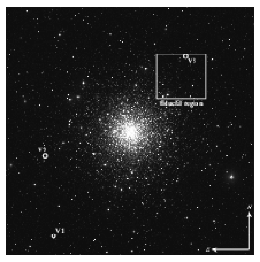
Figure 15: CCD Field of view of M10 with the locations of the variables. The fiducial region is shown for reference. The size of the field of view is 81% (23.5 arcmin on the side) of the area shown in Figures 3, 5, 11, and 13.

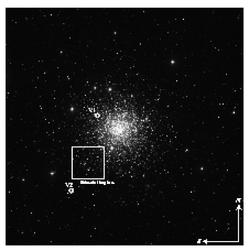
Figure 16: CCD Field of view of M12 with the locations of the variables. The fiducial region is shown for reference. The size of the field of view is 81% (23.5 arcmin on the side) of the area shown in Figures 4, 6, 12, and 14.

Table 6 gives the basic information about the variable stars we detected in the fields of M10 and M12. $V_{bright}$ and $I_{bright}$ are the $V$ and $I$ magnitudes at maximum light. Figures 15 and 16 show the locations of the respective variable stars in the fields of M10 and M12. Figures 9 and 10 indicate where the variables fall within the CMDs of the two clusters. The data shown in Figures 9 and 10 are differentially dereddened to the fiducial region within the respective cluster, as described above. No reddening zero point is applied. The magnitudes and colors of the variables correspond to the values at maximum brightness.

4.3.2 Phased Photometry Lightcurves

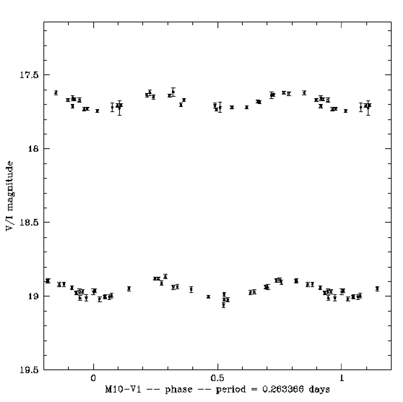
Figure 17: V1 in the field of M10, a W UMa binary system with a period of 0.263366 days. $I$ data are plotted above the $V$ data. No reddening correction is applied to the lightcurve data. M10-V1 is not a member of M10.

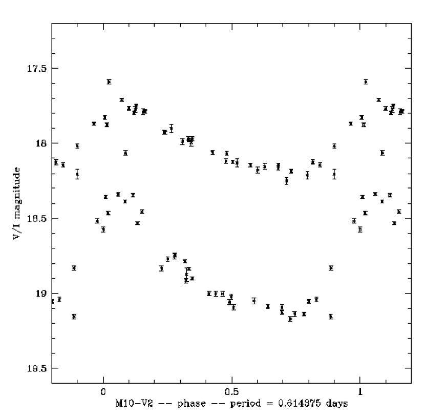
Figure 18: V2 in the field of M10, an RR Lyrae system with a period of 0.61438 days. $I$ data are on top. No reddening correction is applied. The variable is a background star (40 kpc).

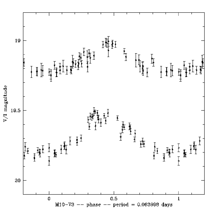
Figure 19: V3 in the field of M10, an SX Phe pulsating variable with a period of 0.0637 days. $V$ data are plotted below the $I$ data. No reddening correction is applied to the lightcurve data. M10-V3 is a background field star (distance $\sim$ 16 kpc).

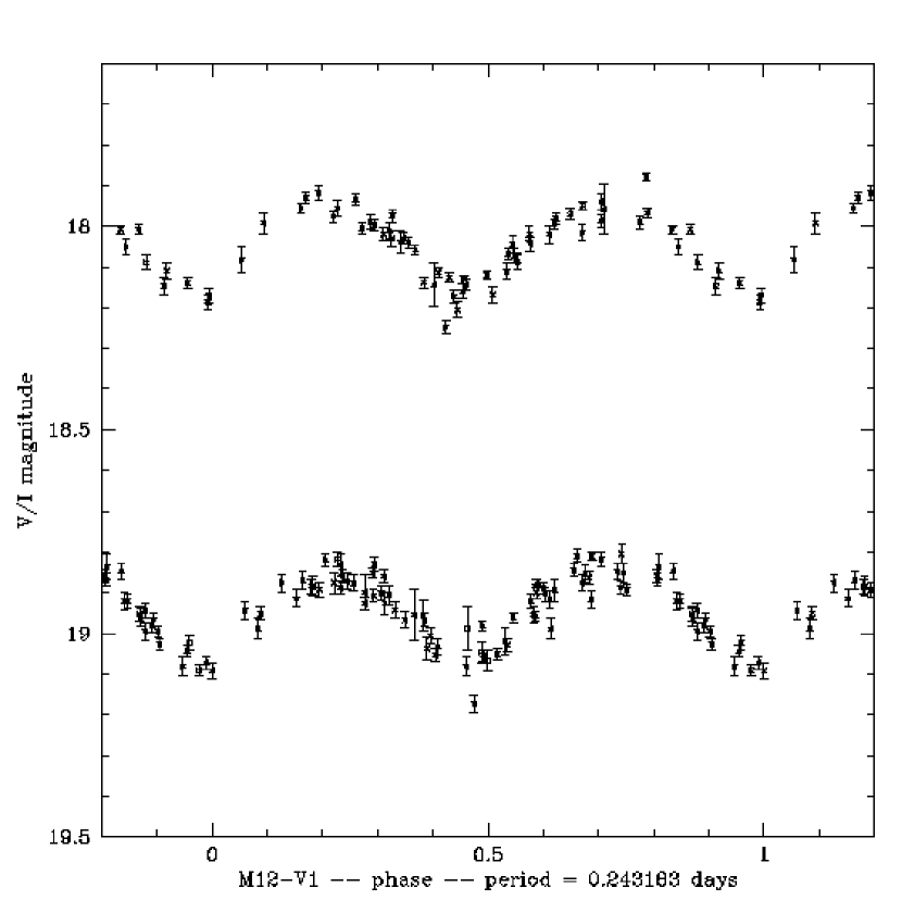
Figure 20: V1 in the field of M12, a W UMa binary system with a period of 0.243183 days and the only variable which is most likely physically associated with a GC. $I$ data are above the $V$ data. No reddening correction is applied to the lightcurve data.

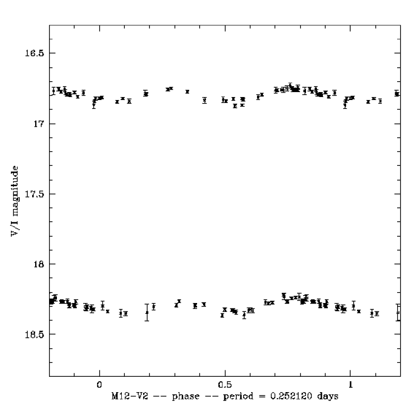
Figure 21: V2 in the field of M12, a W UMa binary system with a period of 0.25212 days. $I$ data are plotted above the $V$ data. No reddening correction is applied to the lightcurve data.

The phased lightcurves for the variable stars are presented in Figures 17 through 21. In particular, Figure 17 shows the lightcurve of M10-V1 (period = 0.263366 days) which is a W Ursa Majoris (W UMa) type contact binary system. M10-V2 is a background RR Lyrae (ab type) variable with a period of 0.61438 days; its lightcurve is displayed in Figure 18. M10-V3 appears to be a field $\delta$ Scuti or an SX Phoenicis-type (SX Phe) variable with a period of 0.0637 days. These stars are rapidly pulsating Population I ($\delta$ Scuti) or Population II (SX Phe) stars which are commonly found towards the faint end of the instability strip in the CMD (Rodriguez, López-González, & López de Coca, 2000). M10-V3’s lightcurve is shown in Figure 19. M12-V1, another W UMa binary, seems to be the only variable in our data set which is physically associated with its respective parent GC (based on its CMD location). Its period is 0.243183 days, and its lightcurve is displayed in Figure 20. M12-V2, another W UMa binary, but not associated with M12, has a period of 0.25212 days; its lightcurve is in Figure 21. In all of these Figures, $V$ data are in the bottom panel, $I$ data in the top panel. The error bars represent the DoPHOT photometric errors associated with that particular measurement of the star’s magnitude. No reddening correction was applied to the lightcurves.

4.3.3 Variable Stars: Distances and Cluster Membership

W UMa Binaries (in M10 and M12)

As indicated in Section 4.3.2, all the binary systems we detect in the fields of M10 and M12 are of the W Ursa Majoris type. W UMa binaries are systems in which the two components are in physical contact with their Roche equipotential lobes and at their inner Lagrangian Point (see, e.g., Rucinski, 1985a, b; Mateo, 1993, for more detailed description of W UMa systems). The fact that the total brightness of the system is constantly changing by up to $\sim$0.75 magnitudes makes them easy to detect. Due to the good thermal contact between the two components, the two stars have similar surface temperatures. The absolute magnitude of the system can therefore be defined as:

$$M_{V}=-4.43\log P+3.63(V-I)_{0}-0.31,$$ (1)

where $M_{V}$ is the absolute $V$ magnitude, $P$ is the period in days, and the $(V-I)_{0}$ color is reddening-free. The empirically determined standard deviation in this relation is $\sigma\sim 0.29$, corresponding to about 13% in distance. See Rucinski (2000) and BM02 for a more detailed derivation of the above equation.

Table 7 shows the absolute magnitudes and distance moduli for the W UMa binaries in the fields of M10 and M12 based on the above relation. The distances to the clusters were calculated in Section 3.2.2 to be 5.1 kpc (M10) and 4.9 kpc (M12). The corresponding true distance moduli (apparent distance moduli corrected for extinction) are $V_{0}-M_{V}=13.55$ and 13.46, respectively. We note that the absolute magnitudes and distance moduli in Table 7 were calculated under the assumption that the W UMa system under investigation is suffering the full extinction between us and the cluster. Since the Rucinski magnitudes for some of the variables indicate that they are foreground stars, this assumption might be incorrect in some cases. That is, for some of the non-members, the color might not be the correct, reddening-free value.

A first indication of whether an EB system in the field of a globular cluster is associated with that cluster is, of course, its location with respect to the cluster center (we note that we cannot study the very center of the cluster due to crowding). The tidal radii of M10 and M12 are 21.48 and 17.6 arcmin, respectively (Harris, 1996). Thus, all the binary systems we find are well within the tidal radii. A more powerful membership criterion is a binary’s location in the CMD. Based on the CMDs of M10 and M12 (see Figures 9 & 10), M10-V1 and M12-V2 are not associated with their respective parent cluster. M12-V1, however, appears to be a cluster member from its location in M12’s CMD. The estimates of distance moduli to the various W UMa binaries in Table 7 confirm what the GC-CMDs suggest: M10-V1 and M12-V2 are foreground stars, but M12-V1 is most likely a member of M12 (it falls well within one $\sigma_{Rucinski}$ of the calculated distance to the GC).

Pulsating Variables (in M10)

The two pulsating variable stars we detected in M10 are M10-V2, an ab-type RR Lyrae star, and M10-V3, either a $\delta$ Scuti or an SX Phe star. From their locations in M10’s CMD, it is apparent that neither of them is associated with the cluster.

Since the “expected” location of any GC-member RR Lyrae is on the horizontal branch, M10-V2 is clearly a background star. If one assumes that $M_{V}\sim 0.7$ for RR Lyraes, M10-V2’s distance is around 40 kpc, putting it into the Milky Way halo beyond the bulge.

As mentioned above, SX Phe stars represent the Population II counterparts to the Pop I $\delta$ Scuti variables (Rodriguez & López-González, 2000). GC-member SX Phe stars are typically found in the blue straggler region of the CMD. Since M10-V3 is not inside this region, we conclude that it is not a member of the GC. Instead, the photometry results for M10-V3 ($\Delta V\sim 0.32$, P $\sim$ 0.064 days, $(V-I)_{0}\sim 0.29$) quite exactly correspond to the modes in the distributions of the catalogue of field $\delta$ Scuti and SX Phe stars of Rodriguez, López-González, & López de Coca (2000); see their figures 1, 3, & 4. Since the number of known field SX Phe stars is very low (Rodriguez, López-González, & López de Coca, 2000; Rodriguez & López-González, 2000; Jeon et al., 2001) we cannot say for sure whether M10-V3 is a field $\delta$ Scuti or SX Phe variable Jeon et al. (see for example figure 5 in 2001). Since M10-V3 is a background variable, however, and thus located in the halo, we will assume that it is an SX Phe variable. Using the appropriate P-L-[Fe/H] relations in Nemec, Nemec, & Lutz (1994) and Nemec et al. (1995) with an assumed [Fe/H] $\sim$ –1.5, we obtain a distance to M10-V3 of approximately 16 kpc.

5 Summary and Concluding Remarks

The GCs M10 and M12 were monitored for the existence of photometrically variable stars in the magnitude range of approximately $16.5<V<20$ and for periods between roughly 0.05 and 5 days. Observations were conducted over a span of about four years with only relatively few epochs per observing run due to the equatorial locations of the clusters.

During the search for variables, we noticed strong differential reddening effects across the field of M10 (Figure 1) and a similar, but weaker signature across M12 (Figure 2). We correct for this differential reddening by creating extinction maps (Figures 3 and 4). The features visible in these maps are similar to the ones detected by SFD in their dust emissivity maps of the same regions (Figures 11 and 12). Applications of our differential extinction maps to our data significantly improves the appearance of the CMDs of the GCs (Figures 7 and 8), especially in the case of M10.

The $E_{V-I}$ zero points for M10 and M12, which need to be added to the differential $E_{V-I}$ values in the grids of Figures 5 and 6, are 0.23 mag and 0.24 mag, respectively, determined by fitting VDB isochrones to the differentially dereddened data. Since previous reddening estimates for these two GCs vary, especially for M10, our results agree with some literature values but not with others. Specifically, our reddening estimate for M12 agrees well with the SFD maps, whereas our value for M10 falls below the one quoted in SFD ($E_{V-I}\sim 0.389$), but produces by far the best VDB isochrone fit.

Reddening studies like the one presented here may be useful in determining properties of the interstellar medium such as a dependence of $R_{V}$ upon position in the field of view. In addition, they may give insight into the properties and the distribution of the dust along the line of sight. One may argue, for instance, that M10 and M12, since they are so close to each other in the sky, lie behind a common, larger scale “layer” of dust that accounts for the practically identical reddening zero point. M10 seems to fall behind another dust ridge Kennedy, Bates, & Kemp (suggested by, e.g., 1996) causing the additional differential reddening which varies on arcmin scales by tenths of a magnitude. Furthermore, reddening maps such as the ones presented here and in BM01 can give a sense of how small a scale differential extinction in general may vary on, and by how much, perhaps as a function of position in the sky or Galactic latitude. We hope to shed some light on this matter with a similar analysis of the remaining GCs in our sample.

Our search for variable stars in M10 and M12 produced five candidates. In M10, we detected a W UMa binary, an RR Lyrae, and an SX Phe field variable. None of these three systems appears to be physically associated with M10, given their locations in the CMD (Figure 9) and their estimated distances (Table 7 and Section 4.3.3). In M12, we detected two W UMa binary systems, one of which (M12-V1) is most likely a cluster member. Again, we base this estimate on CMD location (Figure 10) and calculated distance moduli (Table 7).

As in the case of NGC 3201 (BM02), we detect a number of foreground and background variables but only one (likely) GC member binary. Both M10 and M12 are at higher Galactic latitude ($\sim 25^{\circ}$) than NGC 3201 ($\sim 8.5^{\circ}$), so the disk contamination is not as significant. The number of total stars which were monitored was only slightly different (27000 for NGC 3201 and 34000 for M10 and M12 combined), but in the case of NGC 3201, we found 14 variables (11 binaries, 1 member), whereas in this work we find 5 variables (3 binaries, 1 probable member). In both studies, cluster-member stars outnumber non-member stars, as may easily be seen in the CMDs of the clusters. Yet the number of non-member binaries we find is much higher than the number of member binaries. It will be interesting to see whether this trend continues in the rest of the GCs in our sample which will be analyzed using the same methods as outlined in this work, BM01, and BM02, or whether NGC 3201, M10, and M12 are merely “special cases”.

Finally, we have shown that we are able to detect binaries of very low amplitude ($\sim 0.07$ mag; BM02) and duty cycle (0.1; BM02) and of short ($\sim 0.13$ days; this work) and long periods (2.85 days; BM02), even when using very different observing techniques for the clusters. Using our existing 1m-class telescope photometry data set of the rest of the GCs in our sample, we should be able to identify binaries and other variables in these clusters (provided they exist) and determine their periods. With the spectroscopic capabilities of modern 8m-class telescopes for follow-up observations, we can determine cluster membership for these variables in the near future.

Table 1: M10 Observations

Date	Telescope	Field-of-View Size	Number of Epochs
April 1996	MDM 1.3m	14.9	4
May 1997	LCO 1m	23.5	29
June 1997	MDM 1.3m	14.9	35
August 1997	LCO 1m	23.5	23
May 1998	LCO 1m	23.5	25
August 1998	MDM 1.3m	17	16
August 1998	LCO 1m	23.5	14
May 1999	MDM 1.3m	17	12

Table 2: M12 Observations

Date	Telescope	Field-of-View Size	Number of Epochs
June 1995	MDM 1.3m	10.6	60
April 1996	MDM 1.3m	14.9	4
May 1997	LCO 1m	23.5	28
June 1997	MDM 1.3m	14.9	39
August 1997	LCO 1m	23.5	18
May 1998	LCO 1m	23.5	22
August 1998	MDM 1.3m	17	16
August 1998	LCO 1m	23.5	8
May 1999	MDM 1.3m	17	10

Table 3: Selected Recent Average $E_{V-I}$ Estimates for M10

$E_{V-I}$	Reference	Method
214 mmag	Burstein & Heiles (1982)	HI/galaxy count maps
426 mmag	Reed, Hesser, & Shawl (1988)	integrated light
371 mmag	Hurley, Richer, & Fahlman (1989)	$UBV$ 2-color diagram
234 mmag	Arribas et al. (1990)	infrared photometry
382 mmag	Harris (1996)	compilation of selected previous results
389 mmag	Schlegel, Finkbeiner, & Davis (1998)	dust IR emissivity maps
279 mmag	this work	VDB isochrone fitting

Note. — All listed literature reddening estimates were obtained by converting $E_{B-V}$ values to $E_{V-I}$ by using $E_{B-V}=0.7273\times E_{V-I}$ and a $R_{V}=3.1$ reddening law (Schlegel, Finkbeiner, & Davis, 1998).

Table 4: Selected Recent Average $E_{V-I}$ Estimates for M12

$E_{V-I}$	Reference	Method
127 mmag	Burstein & Heiles (1982)	HI/galaxy count maps
317 mmag	Sato, Richer, & Fahlman (1989)	$UBV$ 2-color diagram
258 mmag	Harris (1996)	compilation of selected previous results
250 mmag	Schlegel, Finkbeiner, & Davis (1998)	dust IR emissivity maps
249 mmag	this work	VDB isochrone fitting

Note. — All listed literature reddening estimates were obtained by converting $E_{B-V}$ values to $E_{V-I}$ by using $E_{B-V}=0.7273\times E_{V-I}$ and a $R_{V}=3.1$ reddening law (Schlegel, Finkbeiner, & Davis, 1998).

Table 5: Selected Recent Average $E_{V-I}$ Estimates for NGC 3201

$E_{V-I}$	Reference	Method
285 mmag	Cacciari (1984)	RR Lyrae colors
285 mmag	Harris (1996)	compilation of selected previous results
336 mmag	Schlegel, Finkbeiner, & Davis (1998)	dust IR emissivity maps
240 mmag	von Braun & Mateo (2001)	VDB isochrone fitting

Note. — All listed literature reddening estimates were obtained by converting $E_{B-V}$ values to $E_{V-I}$ by using $E_{B-V}=0.7273\times E_{V-I}$ and a $R_{V}=3.1$ reddening law (Schlegel, Finkbeiner, & Davis, 1998, $\lambda_{central}\sim 8100$ Å). They represent the updated values from BM01 where we calculated $E_{B-V}=0.6468\times E_{V-I}$, based on Cardelli, Clayton, & Mathis (1989, $\lambda_{central}\sim 9000$ Å).

Table 6: Variable Stars in the Fields of M10 & M12

Var. No.	type	RA (2000)	Dec (2000)	period (days)	$V_{bright}$	$I_{bright}$
M10-V1	W UMa	16:57:39.15	–4:16:03.9	0.263366(28)	18.890(17)	17.620(19)
M10-V2	RR Lyrae	16:57:41.57	–4:08:24.8	0.61438(23)	18.170(14)	17.650(19)
M10-V3	SX Phe	16:56:48.63	–3:58:35.9	0.0637(41)*	19.538(18)	19.013(33)
M12-V1	W UMa	16:47:22.89	–1:55:35.8	0.243183(15)	18.818(19)	17.949(19)
M12-V2	W UMa	16:47:32.58	–2:03:10.1	0.25212(25)*	18.238(12)	16.750(19)

Note. —

• Errors in parentheses indicate the uncertainty in last two digits.

• Photometry errors are the result of adding in quadrature the DoPHOT photometry error for the instrumental magnitude and the rms of the standard star solution (see BM01).

• The random error in the period corresponds to the full width at half maximum (fwhm) of the peak in the AoV power spectrum corresponding to the correct frequency. For the determination of this error, only $V$ data were used. For the variables M10-V3 and M12-V2, the peak in the power spectrum corresponding to the correct period was assigned essentially the same power as the directly neighboring peak (i.e., it would be hard to pick “by eye” which one is the correct one). In these instances, we estimated the period rms to be the distance between these two neighboring peaks. The two cases are marked by an asterisk.

Table 7: Rucinski Magnitudes and Distance Moduli for W UMa-type Binaries in the Fields of M10 & M12

system	period (days)	$E_{V-I}$	$(V-I)_{0,bright}$	$M_{V(Rucinski)}$	$V_{0}-M_{V}$
M10-V1	0.263366(28)	0.323(07)	0.947	5.695	12.576
M12-V1	0.243183(15)	0.249(04)	0.620	4.661	13.679
M12-V2	0.25212(25)	0.259(03)	1.229	6.802	10.939

.

Note. — Rucinski quotes the scatter in his relation (Rucinski, 1994, 1995) to be 0.29 mag in the calculation of the absolute $V$ magnitudes (corresponding to an uncertainty of approximately 13% in distance). Since this uncertainty is far larger than the quadratic sum of all our random errors, we refrain from a detailed error analysis for the Rucinski magnitudes and distance moduli.

Figure 1: CMD of M10 before applying any extinction correction. The typical symptoms of differential extinction across the field are present: main sequence appears relatively tight where it is approximately parallel to the reddening vector (at $V$ fainter than $\sim 20$), whereas regions more or less perpendicular to the reddening vector, such as the MSTO, the subgiant and giant branches as well as the blue HB, appear broad. As part of the process of combining 600s and 10s exposure data, we set the division at around $V\sim 17-17.5$ where saturation of the deep data sets in.

Figure 2: CMD of M12 before applying any extinction correction. The signatures of differential reddening are much less visible than in M10 (see Fig. 1). The division between the deep (600s) and shallow (10s) photometry data is located around $V\sim 17-17.5$.

Figure 3: Extinction Map for M10. North is up, east is to the left. The size of the entire field is 25.9 arcmin on the side. The darker the color of a subregion, the more extinction is occurring in it (see Figure 5) relative to the fiducial region whose position is shown on the map along with the core radius around the location of the center of the cluster. The coordinate axes $x$ and $y$ correspond to the ones in Figure 5. The average reddening with respect to the fiducial region is $E_{V-I}=68\pm 41$ mmag for the entire field and $E_{V-I}=49\pm 28$ mmag for the inner part of the field (see Figure 5). The size of one pixel in this map ($\Delta x=1$ or $\Delta y=1$) is $\sim 140$ arcsec.

Figure 4: Extinction Map for M12. North is up, east is to the left. The size of the entire field is 25.9 arcmin on the side. The darker the color of a subregion, the more extinction is occurring in it (see Figure 6) relative to the fiducial region whose position is shown on the map along with the core radius around the location of the center of the cluster. The coordinate axes $x$ and $y$ correspond to the ones in Figure 6. The average reddening with respect to the fiducial region is $E_{V-I}=40\pm 58$ mmag for the entire field and $E_{V-I}=9\pm 15$ mmag for the inner part of the field where the errors are considerably smaller (see Figure 6) due to the higher stellar density. The size of one pixel in this map ($\Delta x=1$ or $\Delta y=1$) is $\sim 140$ arcsec.

Figure 14: Graphical Representation of the difference between our extinction map for M12 (Fig. 4) and the SFD Map of the same region (Fig. 12 . The location of the fiducial region is given for reference, the orientation, size, and pixel sizes are the same as in Figures 4 and 6. Darker regions correspond to areas where our map indicates more differential extinction (relative to the fiducial region) than the SFD map. The difference map is featureless except in the regions towards the corner of the image which is evidence for the good spatial agreement between the two maps. The average reddening of the whole field is $E_{V-I}=214\pm 53$ mmag, whereas for only the inner region, it is $E_{V-I}=241\pm 11$ mmag.

References

- Andersen (1991) Andersen, J. 1991, A&A Rev., 3, 91
- Arribas et al. (1990) Arribas, S., Martinez Roger, C., Paez, E., & Caputo, F. 1990, Ap&SS, 169, 45
- Binney & Tremaine (1987) Binney, J., & Tremaine, S. 1987, Galactic Dynamics (Princeton, NJ, Princeton University Press, 1987, 747 p.)
- Burstein & Heiles (1982) Burstein, D. & Heiles, C. 1982, AJ, 87, 1165
- Cacciari (1984) Cacciari, C. 1984, AJ, 89, 231
- Cardelli, Clayton, & Mathis (1989) Cardelli, J. A., Clayton, G. C., & Mathis, J. S. 1989, ApJ, 345, 245
- Clement et al. (2001) Clement, C. M., Muzzin, A., Dufton, Q., Ponnampalam, T., Wang, J., Burford, J., Richardson, A., Roseberry, T., Rowe, J., & Sawyer-Hogg, H. 2001, AJ, 122, 2587
- Gallart et al. (1999) Gallart, C., Freedman, W. L., Mateo, M., Chiosi, C., Thompson, I. B., Aparicio, A., Bertelli, G., Hodge, P. W., Lee, M. G., Olszewski, E. W., Saha, A., Stetson, P. B., & Suntzeff, N. B. 1999, ApJ, 514, 665
- Harris (1996) Harris, W. E. 1996, AJ, 112, 1487
- Hurley, Richer, & Fahlman (1989) Hurley, D. J. C, Richer, H. B., & Fahlman, G. G. 1989, AJ, 98, 2124
- Hut et al. (1992) Hut, P., McMillan, S., Goodman, J., Mateo, M., Phinney, E. S., Pryor, C., Richer, H. B., Verbunt, F., & Weinberg, M. 1992, PASP, 104, 981
- Jeon et al. (2001) Jeon, Y.-B., Kim, S.-L., Lee, H., & Myung, G. L. 2001, AJ, 121, 2769
- Kennedy, Bates, & Kemp (1996) Kennedy, D. C., Bates, B., & Kemp, S. N. 1996, A&A, 309, 109
- Lafler & Kinman (1965) Lafler, K., & Kinman, T. D. 1965, ApJS, 11, 216
- Mateo (1993) Mateo, M. 1993, in ASP Conf. Ser. Vol 53, Blue Stragglers, ed. R. E. Saffer, p. 74
- Mateo (1996) Mateo, M. 1996, ASP Conference Series, Vol. 90, The Origins, Evolution, and Destinies of Binary Stars in Clusters, eds. E. F. Milone and J.-C. Mermilliod, page 21
- McVean et al. (1997) McVean, J. R., Milone, E. F., Mateo, M. & Yan, L. 1997, ApJ, 481, 782
- Monet et al. (1996) Monet, D., Bird, A., Canzian, B., Harris, H., Reid, N., Rhodes, A., Sell, S., Ables, H., Dahn, C., Guetter, H., Henden, A., Leggett, S., Levison, H., Luginbuhl, C., Martini, J., Monet, A., Pier, J., Riepe, B., Stone, R., Vrba, F., Walker, R. 1996, USNO-SA2.0, (U.S. Naval Observatory, Washington DC)
- Nemec et al. (1995) Nemec, J. M., Mateo, M., Burke, M., & Olszewski, E. W. 1995, AJ, 110, 1186
- Nemec, Nemec, & Lutz (1994) Nemec, J. M., Nemec, A. F. N., & Lutz, T. E. 1994, AJ, 108, 222
- Paczyński (1996) Paczyński, B. 1996, invited talk presented at STScI, astro-ph/9608094
- Piotto & Zoccali (1999) Piotto, G. & Zoccali, M. 1999, A&A, 345, 485
- Reed, Hesser, & Shawl (1988) Reed, B. C., Hesser, J. E., & Shawl, S. J. 1988, PASP, 100, 545
- Rodriguez & López-González (2000) Rodriguez, E., López-González, M. J. 2000, A&A, 359, 597
- Rodriguez, López-González, & López de Coca (2000) Rodriguez, E., López-González, M. J., & López de Coca, P. 2000, A&AS, 144, 469
- Rosenberg et al. (2000) Rosenberg, A., Aparicio, A., Saviane, I., and Piotto, G. 2000, A&AS, 145, 451
- Rubenstein (1997) Rubenstein, E. P. 1997, PASP, 109, 933
- Rucinski (1985a) Rucinski, S. M. 1985a, in Interacting Binary Stars, eds. J. E. Pringle & R. A. Wade, Cambridge, Cambridge University Press, p. 85
- Rucinski (1985b) Rucinski, S. M. 1985a, in Interacting Binary Stars, eds. J. E. Pringle & R. A. Wade, Cambridge, Cambridge University Press, p. 113
- Rucinski (1994) Rucinski, S. M. 1994, PASP, 106, 462
- Rucinski (1995) Rucinski, S. M. 1995, PASP, 107, 648
- Rucinski (2000) Rucinski, S. M. 2000, AJ, 120, 319
- Sato, Richer, & Fahlman (1989) Sato, T., Richer, H. B., & Fahlman, G. G. 1989, AJ, 98, 1335
- Schechter, Mateo, & Saha (1993) Schechter, P. L., Mateo, M.,& Saha, A. 1993, PASP, 105, 1342
- Schlegel, Finkbeiner, & Davis (1998) Schlegel, D. J., Finkbeiner, D. P., and Davis, M. 1998, ApJ, 500, 525
- Schwarzenberg-Czerny (1989) Schwarzenberg-Czerny, A. 1989, MNRAS, 241, 153
- Stetson (1996) Stetson, P. B. 1996, PASP, 108, 851
- VandenBerg et al. (2000) VandenBerg, D., Swenson, F., Rogers, F. J., Iglesias, C. A., & Alexander, D. R. 2000, ApJ, 532, 430
- von Braun & Mateo (2001) von Braun, K., & Mateo, M. 2001, AJ, 121, 1522
- von Braun & Mateo (2002) von Braun, K., & Mateo, M. 2002, AJ, 123, 279
- Welch & Stetson (1993) Welch, D. L., & Stetson, P. B. 1993, AJ, 105, 1813