Deconvolution with a spatially-variant PSF

Abstract

Application of deconvolution algorithms to astronomical images is often limited by variations in PSF structure over the domain of the images. One major difficulty is that Fourier methods can no longer be used for fast convolutions over the entire images. However, if the PSF is modeled as a sum of orthogonal functions that are individually constant in form over the images, but whose relative amplitudes encode the PSF spatial variability, then separation of variables again allows global image operations to be used. This approach is readily adapted to the Lucy-Richardson deconvolution algorithm. Use of the Karhunen-Loève transform allows for a particularly compact orthogonal expansion of the PSF. These techniques are demonstrated on the deconvolution of Gemini/Hokupa’a adaptive optics images of the galactic center.

1 INTRODUCTION

The deconvolution of astronomical images becomes tricky when the structure of the point-spread function (PSF) varies significantly over the domain of interest. A constant PSF is generally not a formal requirement for most deconvolution algorithms, but it is a profoundly useful simplification. With a constant PSF, one can quickly perform convolutions over the entire image in the Fourier domain, and the difficult problem of trying to estimate the PSF structure as it varies from point to point is completely avoided. Unfortunately, real astronomical images often do have spatially-variant PSFs. This problem is especially important for adaptive-optics (AO) imagery. Presently, all working AO systems can only correct for atmospheric blurring at the location of the guide star or laser beacon. As one moves away from this location in angle, the correction will degrade rapidly.[1] Traditionally there are two approaches for the deconvolution or analysis of such images.

1. The easiest approach is to sweep the problem under the rug! While it may be facetious to suggest that this as a real solution, it is true that there may be some cases where the PSF structural variations are significant in general, but may be ignored for specific problems. One might imagine a diffraction-limited system in which the form of the sharp core varied over the image, but the broad wings more or less stayed the same; for some problems, the latter component of the PSF may be more important.

2. Break the image up into many sub-domains, over which the PSF may be regarded as constant. This procedure is tedious at best, may produce discontinuities when the sub-images are stitched back together, and still must find a way to represent the PSF satisfactorily at all the locations demanded.

In this paper, I will outline a different approach that incorporates the continuous variation of the PSF into the deconvolution, but that also uses efficient full-image Fourier convolution; in this regard, it should be superior to, but yet simpler than the sub-domain approach. As it happens, this method simply strings together ideas already in the literature for compactly modeling the PSF spatial variations, as well as encoding the variations in a form that allows for efficient convolution. Folding these methods into standard Lucy[2]-Richardson[3] deconvolution allows that algorithm to work quickly with a variable PSF; this method is readily adopted, as it actually only incorporates forward convolutions of the PSF (and its transpose) to estimate the deconvolved image.

An important caveat is that while a spatially-variant PSF deconvolution algorithm attempts to use the most accurate PSF possible for any point in the image, this does not imply that the deconvolved image will have uniform resolution. Although a forward convolution of a source model to match an image with large PSF variations may be readily done, with real image noise the resolution gains offered by deconvolution of such images will always be tied to the intrinsic resolution of the local PSF. In the single-point AO case, for example, one will not be able to deconvolve the entire image to the same fine resolution available at the correction-point. Variable-PSF deconvolution cannot undo any real loss of structural information that occurs as the resolution degrades away from the reference point.

2 THEORY

2.1 Encoding the PSF Spatial Variability

The critical step in deconvolution of a spatially-variant PSF is to understand how ordinary convolution can be done efficiently with a variable PSF. This methodology can then just be folded in to those deconvolution algorithms, such as Lucy-Richardson, that are based on forward convolution. This discussion is thus limited to how to treat the variable PSF, rather than the actual deconvolution algorithm itself.

If we ignore noise for this discussion, then an astronomical image, $I,$ can be presented schematically as the convolution of an astronomical source, $S,$ and a PSF, $P:$

$$I=S*P.$$ (1)

In the general case of a PSF that varies with location over the image, this equation can be expanded explicitly as:

$$I(x,y)=\int_{-\infty}^{\infty}\int_{-\infty}^{\infty}S(u,v)~{}P(u,v,x-u,y-v)~{}du~{}dv,$$ (2)

where $\{x,y\}$ are any pixel location in the image and $\{u,v\}$ are the pixel locations in the source. The PSF is assumed to have a form that changes with $\{u,v\}.$ The key step is to recast the PSF as a sum of orthogonal functions, each of which is constant over the domain, but whose varying amplitudes serve to encode the PSF spatial variance. This gives

$$P(u,v,x,y)=\sum_{i=1}^{\infty}a_{i}(u,v)~{}p_{i}(x,y),$$ (3)

where $\{p_{i}\}$ are of the orthogonal PSF components, and $\{a_{i}\}$ is a field that specifies how the amplitudes of $\{p_{i}\}$ varies over the image domain to describe overall variations in the PSF. This representation allows the variables to be separated in the convolution, [4, 5, 6]

$$I(x,y)=\sum_{i=1}^{\infty}\int_{-\infty}^{\infty}\int_{-\infty}^{\infty}S(u,v)~{}a_{i}(u,v)~{}p_{i}(x-u,y-v)~{}du~{}dv.$$ (4)

In other words, each PSF component can be convolved with the source weighted by a coefficient field over its full domain, which is easily done in the fourier domain, to make an image component. The image components are then summed to make the final complete image. Provided that the $\{a_{i}\}$ are known in advance, the computational burden of tracking the PSF variability scales only linearly with the number of PSF components over that required for a constant-PSF convolution.

2.2 Karhunen-Loève PSF Decomposition

Choice of the appropriate PSF basis functions, $\{p_{i}\},$ is critical to the ease of computing $\{a_{i}\}$ as well minimizing as the computational overhead associated with computing equation (3). Of the large set of basis functions that one might contemplate, Karhunen-Loève decomposition of the PSF appears to offer an attractive solution to both problems; it is presently used by the Sloan Digital Sky Survey to characterize PSF variations[7]. Karhunen-Loève decomposition is closely related to principal-component analysis. It works by finding the most important eigenvectors that describe the space spanned by a set of objects. It is non-parametric and by maximizing the variance accounted for by each eigenvector, effectively minimizes the total dimension of the basis.

Calculation of the Karhunen-Loève decomposition is simple. If one has a set of $N$ PSF observations, $P^{*}_{i},$ distributed of an image domain, one first normalizes the PSFs to a common integral, spatial extent, and photocenter to remove such trivial variations from the problem. A covariance matrix between all the PSFs is then computed, with

$$C_{ij}=<P^{*}_{i}\ P^{*}_{j}>.$$ (5)

The eigenvalues, $\lambda_{i},$ of this matrix are then found; the corresponding eigenvectors, $\{x_{i}\},$ define the PSF basis functions or “eigen-PSF” images:

$$p_{i}=\sum_{1=1}^{N}x_{ij}P^{*}_{j},$$ (6)

where $x_{ij}$ is component $j$ of $x_{i}.$ One thus directly derives the basis function from the data itself without recourse to any parametric forms. The importance of any $x_{i}$ for characterizing the span of $\{P^{*}\}$ is given by the amplitude of its corresponding eigenvalue. If the $\{p_{i}\}$ are sorted by the eigenvalue amplitude, then the one can assess how many terms are really required to explain the significant structure in the PSF observations. Use of all $N$ eigen-PSFs will fit each observation exactly, including noise. It is likely instead that a subset of $K$ eigen-PSFs will be sufficient. The attractiveness of the Karhunen-Loève decomposition method is that since it each eigen-PSF corresponds to a principal axis in the space spanned by the PSF observations, some of the less significant dimensions may be neglected, potentially allowing for $K<<N.$

With the Karhunen-Loève decomposition in hand, one immediately has the decomposition of $\{P^{*}\},$ into the form specified by equation (3), with the exception that the sum is completed at $N$ terms, rather than being infinite; as noted, it may be truncated further by discarding nonsignificant eigen-PSFs. The final step, is to model the behavior of $\{a_{i}\}$ over the image domain so they can expressed as continuous coefficient fields. Unlike the decomposition of the PSF observations, themselves, this step may require fitting a parametric form or model to the coefficients as a function of position within the image domain. Choice of this model may be driven by the context. For AO observations, for example, the PSFs broaden as function of radial distance from the reference point and may have anisotropic shapes that are related to the direction vector to the reference point. In this case, it’s natural to express the coefficient fields in functions of polar coordinates.

The main caveat with the use of Karhunen-Loève decomposition coupled to a model of the coefficient fields is that it provides only an approximation to the true PSF at any point in the image domain. Since in general, one is likely to use some observational representation of the PSF for any deconvolution problem, then it is possible that this issue in this context presents no more additional burden that that always required to understand how dependent the analysis of the deconvolved image is on errors in the PSF. That said, there are two concerns specifically related to use of Karhunen-Loève decomposition.

1. For many deconvolution algorithms, the PSF must be positive definite. Even if a truncated Karhunen-Loève decomposition is always positive definite at the locations of the $\{P^{*}\},$ does not mean that the coefficient fields guarantee this to be true at all other image locations, particularly near the image margins, where the modeled PSF is likely to be an extrapolation. Solution to this problem, if it occurs, may be related to the way the coefficients fields are modeled. In practice, if the span of $\{P^{*}\}$ is limited, then the first eigen-PSF will strongly resemble an average PSF, with the next eigen-PSFs characterizing variations about this form sufficiently limited that the total PSF remains positive definite.

2. A more important problem is that the Karhunen-Loève decomposition is certainly not likely to preserve the unit-integral of the PSFs. Fortunately this problem is simply solved by normalizing equation (3) by the convolution of the PSF with a field of unit amplitude.[5] This gives the Karhunen-Loève approximated PSF at any location as

   $$P_{KL}(u,v,x,y)=\sum_{i=1}^{K}a_{i}(u,v)~{}p_{i}(x,y)~{}\bigg{/}~{}\sum_{i=1}^{K}~{}\int_{-\infty}^{\infty}\int_{-\infty}^{\infty}~{}a_{i}(u,v)~{}p_{i}(x-u,y-v)~{}du~{}dv.$$ (7)

   In practice, the denominator will be a single “normalization image” that can either be used to scale the coefficient fields in advance, or applied to any convolution after the fact as a sort of flat-field.

2.3 The Lucy-Richardson Deconvolution Algorithm

Lucy-Richardson deconvolution works by iteratively comparing an estimate of the intrinsic astronomical source with its image. The first iterative step begins can begin with any initial estimate of the source structure based on prior information, although in practice most users of this method start with a constant level over the entire source domain. At any iterative cycle, $n,$ the running estimate of the source is convolved with the PSF

$$I_{n}=S_{n}*P,$$ (8)

to make an estimate of the true image. A correction image is then estimated by convolving a ratio of the true to estimated image by the transpose of the PSF,

$$C_{n}=\left({I\over I_{n}}\right)*P^{T}.$$ (9)

This is used to update the source estimate by multiplication,

$$S_{n+1}=C_{n}S_{n}$$ (10)

For each Lucy-Richardson iteration thus requires one convolution of the PSF with the source, and one convolution of the image to estimated-image ratio with the PSF transpose. The first step has already been given in equation (4); the second step only requires substituting $\{p_{i}^{T}\}$ for $\{p_{i}\},$ noting that this step still uses the same $\{a_{i}\}.$ Using Lucy-Richardson for a variable PSF is thus conceptually simple, although it does require more complex “book keeping” and indexing to keep track of the various sets of PSF components, coefficient fields, and their normalization.

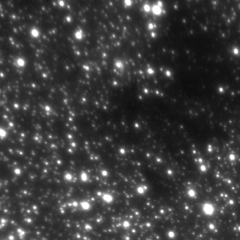
Figure 1: An H-band image of a galactic center starfield obtained with the QUIRC/Hokupa’a AO camera is shown. It was obtained under the Gemini Galactic Center Demonstration Science Program and is publicly available from the Gemini website http://www.gemini.edu. The AO guidestar is just outside the right edge of the image near the lower corner. The area shown is $20.7\times 20.7$ arcsecond. A linear stretch has been used.

3 DEMONSTRATION

Figure 1 shows an H-band images of a star field close to the galactic center obtained with the QUIRC/Hokupa’a AO Camera at the Gemini-N 8m telescope. The AO guidestar is located near the lower-right corner of the image. Stars at this location are compact and round, but become more elongated and broader as the angular offset from the guidestar increases. Several of the brighter stars were drawn from the image to characterize the PSF variation. The Karhunen-Loève decomposition produces the eigen-PSFs shown in Figure 2. In general, the eigen-PSFs

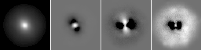
Figure 2: The first four eigen-PSFs for the galactic center starfield are shown. The most significant eigen-PSF is at the left, and is positive definite. The next eigen-PSFs are shown in order of decreasing significance. They have both positive and negative components; the zero level is shown at the margins. Stretches are arbitrary for each eigen-PSFs and thus do not reflect their relative significance. Each subimage is 1.28 arcseconds on a side.

need not correspond to any simple description of how the PSFs vary, but in this case the role of the most important of the set are fairly obvious. The dominant eigen-PSF, as discussed above, looks very much like a simple average over the stars. The second eigen-PSF is clearly moderating the width of the PSF, but because for this image width correlates with elongation, it is not circularly symmetric as a simple pure-width term would be. In passing, this raises an important caveat in the use of Karhunen-Loève decomposition. Since the eigen-PSFs are determined directly by the span of the data, they will vary as the PSF sample is varied. Continuing on, the third eigen-PSF appears to control the orientation of the PSF, while the final eigen-PSF shown in part appears to be describing the PSF wings at large angle. The next eigen-PSFs (not shown) become more complex, but less significant and begin describing the image noise of the PSF samples. Figure 3 shows that using just four eigen-PSFs provides an excellent description of the PSFs and their variability.

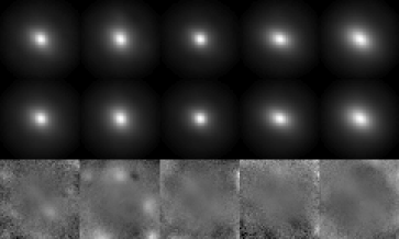
Figure 3: The top line shows images of five of the sample PSFs and the middle line shows the model PSFs using just the first four eigen-PSFs. The bottom line of subimages shows the observed-model differences.

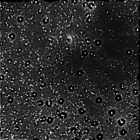
Figure 4: The field shown in Figure 1 has been deconvolved with 160 Lucy-Richardson iterations, using the spatially-variant PSF. The stretch is the same.

The Lucy-Richardson deconvolution (160 iterations) of the galactic center star-field is shown in Figure 4, starting with a constant image as the initial starting point. One of the attractive feature of the Lucy-Richardson method is that since it’s based on simple arithmetic operations in the image and Fourier domain, it’s simple to implement at the high level in any image processing system that emphasizes easy use of such atomic operations. I’ve long used Lucy-Richardson only implemented as a high-level command-language program in the Vista image processing system. Augmentation of this program to implement a spatially-variant PSF deconvolution of Lucy-Richardson was simple; speed is emphasized over memory resources by preserving the Fourier transforms of the eigen-PSFs and their transposes, which only need to be calculated once during the initialization of the deconvolution.

At this writing, I’m just beginning to experiment with this method, but Figure 5 is offered as a comparison of the difference between assuming a constant PSF, and allowing it to vary. The deconvolution on the left used a PSF obtained close to the AO guide star, the image on the right allows the PSF to vary. The right image shows greater amplification of the stars, but a reduction in their strong elongation. Again, emphasizing the point made in the introduction, this elongation cannot be completely erased, but by using a PSF that is appropriate for the field is has been reduced as well as the native Lucy-Richardson algorithm will allow. Future work will be to apply this method to other AO datasets and HST images as well.

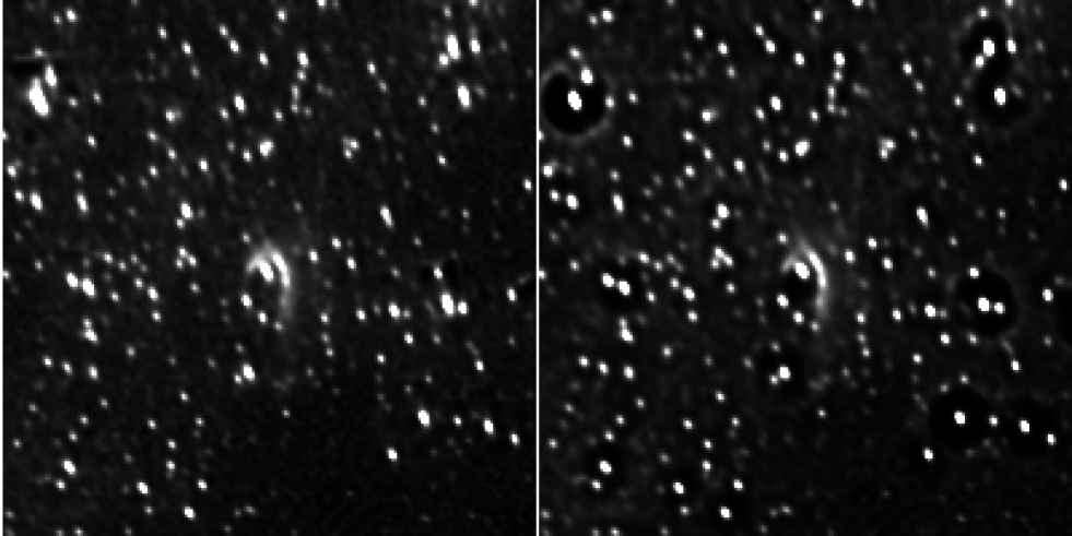
Figure 5: This figure shows shows the deconvolution of the portion of the field centered on the IRS8 source (a star with an associated ISM bowshock) to demonstrate the differences between two deconvolutions done on the assumption of a constant PSF (left) and spatially-variant PSF (right).

- [1] E. Steinbring, S. M. Faber, S. Hinkley, B. A. Macintosh, D. Gavel, E. L. Gates, Julian C. Christou, M. Le Louarn, L. M. Raschke, S. A. Severson, F. Rigaut, D. Crampton, J. P. Lloyd, and J. R. Graham, “Characterizing the Adaptive Optics Off-Axis Point-Spread Function - I: A Semi-Empirical Method for Use in Natural-Guide-Star Observations,” Proc. Astron. Soc. Pac., in press, 2002.
- [2] L. B. Lucy, “An Iterative Technique for the Rectification of Observed Distributions,” Astron. J., 79, pp. 745-754, 1974.
- [3] W. H. Richardson, “Bayesian-Based Iterative Method of Image Restoration,” J. Opt. Soc. Am., 62, pp. 55-59, 1972.
- [4] T. G. Stockham, “High Speed Convolution and Correlation,” Spring Joint Computer Conference, AFIPS Proc., 28, pp. 229-233, 1966.
- [5] C. Alard, “Image Subtraction Using a Space-Varying Kernel,” Astron. Astroph. Sup.,, 144, pp. 363-370, 2000.
- [6] J. Kepner, “A Multi-Threaded Fast Convolver for Dynamically Parallel Image Filtering,” J. Parallel and Distributed Computing, in press, 2002.
- [7] R. H. Lupton, J. E. Gunn, Z. Ivezic, G. R. Knapp, S. Kent, and N. Yasuda, “The SDSS Imaging Pipelines,” in Astronomical Data Analysis Software and Systems X, F. R. Harnden, Jr., F. A. Primini, and H. E. Payne, ed., Astron. Soc. Pac. Conf. Proc., 238, pp. 269-278, 2001.