X-ray spectral variability signatures of flares in BL Lac objects

Abstract

We are presenting a detailed parameter study of the time-dependent electron injection and kinematics and the self-consistent radiation transport in jets of intermediate and low-frequency peaked BL Lac objects. Using a time-dependent, combined synchrotron-self-Compton and external-Compton jet model, we study the influence of variations of several essential model parameters, such as the electron injection compactness, the relative contribution of synchrotron to external soft photons to the soft photon compactness, the electron-injection spectral index, and the details of the time profiles of the electron injection episodes giving rise to flaring activity. In the analysis of our results, we focus on the expected X-ray spectral variability signatures in a region of parameter space particularly well suited to reproduce the broadband spectral energy distributions of intermediate and low-frequency peaked BL Lac objects. We demonstrate that SSC- and external-Compton dominated models for the $\gamma$-ray emission from blazars are producing significantly different signatures in the X-ray variability, in particular in the soft X-ray light curves and the spectral hysteresis at soft X-ray energies, which can be used as a powerful diagnostic to unveil the nature of the high-energy emission from BL Lac objects.

1 Introduction

The class of objects referred to as blazars consists of the most extreme examples of active galactic nuclei (AGNs), namely $\gamma$-ray loud, flat-spectrum radio quasars (FSRQs), and BL Lac objects. They have been observed in all wavelength bands — from radio through very-high energy (VHE) $\gamma$-ray frequencies. More than 65 blazars have been identified as sources of $>100$ MeV emission detected by the EGRET telescope on board the Compton Gamma-Ray Observatory (CGRO) (Hartman et al., 1999), and at least 6 blazars have now been detected at VHE $\gamma$-rays ($>350$ GeV) by ground-based air Čerenkov telescopes (for a recent review see, e.g., Buckley (2001)). Blazars exhibit variability at all wavelengths (von Montigny et al., 1995; Mukherjee et al., 1997) on time scales — in some cases — down to less than an hour (Gaidos et al., 1996).

The broadband continuum spectra of blazars are dominated by non-thermal emission and consist of at least two clearly distinct, broad spectral components. A sequence of sub-classes of blazars can be defined through increasing peak frequencies and a decreasing dominance of the $\gamma$-ray output in terms of $\nu F_{\nu}$ peak flux along a sequence from FSRQs via low-frequency BL Lac objects (LBLs) to high-frequency peaked BL Lac objects (HBLs), which is also correlated with a decreasing inferred bolometric luminosity of the sources (Fossati et al., 1998). For recent reviews of the observational properties of blazars see, e.g., Sambruna (2000), Padovani & Urry (2001), or Böttcher (2002).

Although all extragalactic sources detected by ground-based air Čerenkov telescope facilities to date are HBLs, the steadily improving flux sensitivities and decreasing energy thresholds of those instruments provide a growing potential to extend their blazar source list towards intermediate and even low-frequency peaked BL Lac objects. The detection of such objects at energies $\sim 40$ – 100 GeV might provide an opportunity to probe the intrinsic high-energy cutoff of their spectral energy distributions (SEDs) since at those energies, $\gamma\gamma$ absorption due to the intergalactic infrared background is expected to be negligible at redshifts of $z\lesssim 0.2$ (de Jager & Stecker, 2002). Such detections should significantly further our understanding of the relevant radiation mechanisms responsible for the high-energy emission of blazars and the underlying particle acceleration mechanisms.

The low-energy component of blazar SEDs is well understood as synchrotron emission from ultrarelativistic electrons in a relativistic jet directed at a small angle with respect to the line of sight. In the framework of leptonic models (for a review of the alternative class of hadronic jet models, see, e.g., Rachen (2000)), high-energy emission will result from Compton scattering of lower-frequency photons off the relativistic electrons. Possible target photon fields for Compton scattering are the synchrotron photons produced within the jet (the SSC process; Marscher & Gear (1985); Maraschi, Ghisellini, & Celotti (1992); Bloom & Marscher (1996)), or external photons (the EC process). Sources of external seed photons include the UV – soft X-ray emission from the disk — either entering the jet directly (Dermer, Schlickeiser, & Mastichiadis, 1992; Dermer & Schlickeiser, 1993) or after reprocessing in the broad line region (BLR) or other circumnuclear material (Sikora, Begelman, & Rees, 1994; Blandford & Levinson, 1995; Dermer, Sturner, & Schlickeiser, 1997) —, jet synchrotron radiation reflected at the BLR (Ghisellini & Madau, 1996; Bednarek, 1998; Böttcher & Dermer, 1998), or the infrared emission from circumnuclear dust (Bla$\dot{\rm z}$ejowski et al., 2000; Arbeiter, Pohl, & Schlickeiser, 2002).

According to the now well-established AGN unification scheme (Urry & Padovani, 1995), blazars can be unified with other classes of AGN, in particular radio galaxies, through orientation effects. However, Sambruna, Maraschi, & Urry (1996) have pointed out that such orientation effects can not explain the differences between different blazar sub-classes. Instead, it has been suggested that the sequence of spectral properties of blazars from HBLs via LBLs to FSRQs can be interpreted in terms of an increasing total power input into non-thermal electrons in the jet, accompanied by an increasing contribution of external photons to the seed photon field for Compton upscattering (Madejski, 1998; Ghisellini et al., 1998). It has been suggested that this may be related to an evolutionary effect due to the gradual depletion of the circumnuclear material being accreted onto the central black hole (D’Elia & Cavaliere, 2000; Cavaliere & D’Elia, 2002; Böttcher & Dermer, 2002). Detailed modeling of blazars in the different sub-classes (FSRQs, LBLs and HBLs) seems to confirm this conjecture (for a recent review, see, e.g., Böttcher (2002)).

As mentioned earlier, blazars tend to exhibit rapid flux and spectral variability. The variability is most dramatic and occurs on the shortest time scales at the high-energy ends of the two nonthermal spectral components of their broadband SEDs. Particularly interesting variability patterns could be observed at X-ray energies for those blazars whose X-ray emission is dominated by synchrotron emission. Observational studies of X-ray variability in blazars have so far focused on HBLs and, in particular, on the attempt to identify clear patterns of time lags between hard and soft X-rays. However, such studies have yielded rather inconclusive and often contradictory results (e.g., for Mrk 421: Takahashi et al. (1996); Fossati et al. (2000); Takahashi et al. (2000); or PKS 2155-304: Chiapetti et al. (1999); Zheng et al. (1999); Kataoka et al. (2000); Edelson et al. (2001)). Instead, the so-called “spectral hysteresis” of blazar X-ray spectral variability may prove to be a more promising diagnostic of the physical nature of acceleration and cooling processes in blazar jets: When plotting the X-ray spectral hardness vs. the X-ray flux (hardness-intensity diagrams = HIDs), some HBLs (e.g., Mrk 421 and PKS 2155-304) have been observed to trace out characteristic, clockwise loops (Takahashi et al. (1996); Kataoka et al. (2000)). In terms of pure SSC jet models, such spectral hysteresis can be understood as the synchrotron radiation signature of gradual injection and/or acceleration of ultrarelativistic electrons into the emitting region, and subsequent radiative cooling (Kirk, Rieger, & Mastichiadis, 1998; Georganopoulos & Marscher, 1998; Kataoka et al., 2000; Kusunose, Takahara, & Li, 2000; Li & Kusunose, 2000). However, interestingly, such spectral hysteresis could not be confirmed in a recent series of XMM-Newton observations of Mrk 421 (Sembay et al., 2002).

In LBLs, the soft X-ray emission is also sometimes dominated by the high-energy end of the synchrotron component (Tagliaferri et al., 2000; Ravasio et al., 2002), so similar spectral hysteresis phenomena should in principle be observable. However, those objects are generally much fainter at X-ray energies than their high-frequency peaked counterparts, making the extraction of time-dependent spectral information an observationally very challenging task (see, e.g., Böttcher et al. (2002)), which may require the new generation of X-ray telescopes such as Chandra or XMM-Newton. Extracting the physical information contained in the rich X-ray variability patterns exhibited by BL Lac objects requires detailed theoretical modeling of the time-dependent particle acceleration and radiation transport processes in the jets of blazars. Previous analyses of these processes (Kirk, Rieger, & Mastichiadis, 1998; Georganopoulos & Marscher, 1998; Chiaberge & Ghisellini, 1999; Kataoka et al., 2000; Kusunose, Takahara, & Li, 2000; Li & Kusunose, 2000; Krawczynski, Coppi, & Aharonian, 2002) have led to significant progress in our understanding of the particle acceleration and radiation mechanisms in HBLs, but were restricted to pure SSC models, with parameter choices specifically targeted towards HBLs. Consequently, those results may not be directly applicable to intermediate or low-frequency peaked BL Lac objects or even FSRQs. A notable exception is a recent study by Sikora et al. (2001) (see also Moderski, Bla$\dot{\rm z}$ejowski, & Sikora (2002)), who included a significant contribution of external Compton radiation to the high-energy emission of blazars, and focused on the modeling of photon-energy dependent light curves and time lags between different frequency bands. They applied their results to the FSRQ 3C 279, and concluded that the correlated X-ray/$\gamma$-ray variability of this quasar was inconsistent with X-rays and $\gamma$-rays being produced by the same radiation mechanism because otherwise significant systematic time lags between the $\gamma$-ray and X-ray flaring behaviour would be expected, contrary to the observations (e.g., Hartman et al. (2001)).

In the present paper, we describe a newly developed combined SSC + ERC jet radiation transfer code, accounting for time-dependent particle acceleration and injection, radiative cooling, and escape, coupled to the self-consistent treatment of the relevant photon emission, absorption, and escape processes. In §2 we give a brief description of the underlying blazar jet model. The numerical procedure used in our code will be outlined in §3. We present results of a detailed parameter study, relevant for application to intermediate and low-frequency peaked BL Lac objects, in §4. We summarize in §5.

2 Model Description

The blazar model used for this study is a generic leptonic jet model. It is assumed that a population of ultrarelativistic, non-thermal electrons (and positrons) is injected at a generally time-dependent rate into a spherical emitting volume of co-moving radius $R_{b}$ (the “blob”). The injected pair population is specified through an injection power $L_{\rm inj}(t)$ and the spectral characteristics of the injected non-thermal electron distribution. We assume that electrons are injected with a single power-law distribution with low and high energy cutoffs $\gamma_{1}$ and $\gamma_{2}$, respectively, and a spectral index $q$ so that the injection function $Q_{e}(\gamma;t)$ [cm^-3 s^-1], in the co-moving frame of the emitting region, is

$$Q_{e}^{\rm inj}(\gamma;t)=Q_{0}^{\rm inj}(t)\,\gamma^{-q}\;\;{\rm for}\;\;\gamma_{1}\leq\gamma\leq\gamma_{2}$$ (1)

with

$$Q_{0}^{\rm inj}(t)=\cases{{L_{\rm inj}(t)\over V^{\prime}_{b}\,m_{e}c^{2}}\,{2-q\over\gamma_{2}^{2-q}-\gamma_{1}^{2-q}}&if $q\neq 2$\cr\cr{L_{\rm inj}(t)\over V^{\prime}_{b}\,m_{e}c^{2}\,\ln(\gamma_{2}/\gamma_{1})}&if $q=2$,\cr}$$ (2)

where $V^{\prime}_{b}$ is the blob volume in the co-moving frame.

The jet is powered by accretion of material onto a supermassive central object, which is accompanied by the formation of an accretion disk. For the purpose of this study, we have represented the disk by a standard Shakura-Sunyaev disk with a bolometric luminosity of $L_{D}=10^{45}$ ergs s^-1. The choice of this and several other standard parameters is motivated by a recent modeling study of the LBL W Comae (Böttcher, Mukherjee, & Reimer, 2002). The randomly oriented magnetic field $B$ is determined by an equipartition parameter $\epsilon_{B}$, which is the fraction of the magnetic field energy density $u_{B}$ compared to its value for equipartition with the relativistic electron population in the emission region. As a consequence of this parametrization, the magnetic field will gradually change throughout the evolution of the blob as particles are being injected and subsequently cool along the jet. The blob moves with relativistic speed $v/c=\beta_{\Gamma}=\sqrt{1-1/\Gamma^{2}}$ along the jet which is directed at an angle $\theta_{\rm obs}$ (with $\mu\equiv\cos\theta_{\rm obs}$) with respect to the line of sight. The Doppler boosting of emission from the co-moving to the observer’s frame is determined by the Doppler factor $D=\left[\Gamma\,(1-\beta\mu)\right]^{-1}$.

As the emission region moves outward along the jet, particles are continuously injected according to Eq. 1, are cooling, primarily due to radiative losses, and may leak out of the system. We parametrize particle escape through an energy-independent escape time scale $t_{\rm esc}=\eta\,R_{b}/c$ with $\eta\geq 1$. This parametrization of particle escape can also be used to include adiabatic losses, which are not explicitly taken into account in our simulations. Radiation mechanisms included in our simulations are synchrotron emission, Compton upscattering of synchrotron photons (SSC = Synchrotron Self Compton scattering), and Compton upscattering of external photons (EC = External Compton scattering), including photons coming directly from the disk as well as re-processed photons from the broad line region. The broad line region is modelled as a spherical shell between $r_{\rm BLR,in}=0.2$ pc and $r_{\rm BLR,out}=0.25$ pc (we note, however, that the details of the radial distribution of the BLR material do not play an important role as long as $r_{\rm BLR,out}-r_{\rm BLR,in}\lesssim r_{\rm BLR,in}$), and a radial Thomson depth $\tau_{\rm T,BLR}$ which is considered a free parameter. $\gamma\gamma$ absorption and the corresponding pair production rates are taken into account self-consistently, using the general solution for the pair production rate of Böttcher & Schlickeiser (1997). However, in all simulations presented in this paper, the $\gamma\gamma$ opacity is $\ll 1$ out to at least several tens of GeV so that $\gamma\gamma$ absorption and pair production do not play an important role. Motivated by the $\sim 10$ hr minimum variability time scale observed in W Comae (Tagliaferri et al., 2000), we choose $R_{b}=10^{16}$ cm, and $\Gamma=D=10$, which implies $\theta_{\rm obs}=5.74^{o}$.

Based on an equipartition parameter $\epsilon_{B}\sim 1$, we expect typical magnetic field values of order $B\sim 1$ G (Böttcher, Mukherjee, & Reimer, 2002), which implies a synchrotron cooling time scale (in the observer’s frame) of electrons emitting synchrotron radiation at an observed energy $E_{\rm sy}=1\,E_{\rm keV}$ keV of

$$\tau_{\rm sy}\approx 0.29\,\left({B\over 1\,{\rm G}}\right)^{-3/2}\,\left({D\over 10}\right)^{-1/2}\,E_{\rm keV}^{-1/2}\;{\rm hr}.$$ (3)

For X-ray photon energies, this is shorter than the dynamical time scale $R_{B}/(D\,c)$, in agreement with the approximately symmetric shape of the X-ray light curves generally observed both in W Comae (Tagliaferri et al., 2000) and BL Lacertae (Ravasio et al., 2002).

3 Numerical Procedure

In order to treat the time-dependent electron dynamics and radiation transfer problem in the emitting volume, we solve simultaneously the kinetic equation for the relativistic electrons,

$${\partial n_{e}(\gamma,t)\over\partial t}=-{\partial\over\partial\gamma}\left(\left[{d\gamma\over dt}\right]_{\rm loss}\,n_{e}[\gamma,t]\right)+Q_{e}(\gamma,t)-{n_{\rm e}(\gamma,t)\over t_{\rm e,esc}},$$ (4)

and for the photons,

$${\partial n_{\rm ph}(\epsilon,t)\over\partial t}=\dot{n}_{\rm ph,em}(\epsilon,t)-\dot{n}_{\rm ph,abs}(\epsilon,t)-{n_{\rm ph}(\epsilon,t)\over t_{\rm ph,esc}}.$$ (5)

Here, $(d\gamma/dt)_{\rm loss}$ is the radiative energy loss rate for the electrons, $Q_{e}(\gamma,t)$ is the sum of the external injection rate $Q_{e}^{\rm inj}$ from Eq. 1 and the intrinsic $\gamma\gamma$ pair production rate, $\dot{n}_{\rm ph,em}(\epsilon,t)$ and $\dot{n}_{\rm ph,abs}(\epsilon,t)$ are the photon emission and absorption rates corresponding to the various radiation mechanisms, and $t_{\rm ph,esc}=(3/4)\,R_{b}/c$. In Eq. 4, electron cooling is approximated as a continuous function of time (i.e., the energy of an individual electron is described as a differentiable function of time). This would be inaccurate if a significant contribution to the cooling rate were due to Compton scattering in the Klein-Nishina limit since in that case, the electron is transferring virtually all of its energy to a soft photon in a single scattering event. However, in the parameter ranges which we are primarily interested in, electron cooling is dominated by synchrotron losses and Compton scattering in the Thomson regime, for which Eq. 4 is a good approximation. In Eq. 5, the emissivity term contains the contribution from Compton scattering into a given photon energy interval. Since in all model situations considered here, the Thomson depth of the emitting region is $\tau_{\rm T}\ll 10^{-6}$, the modification of the photon spectrum due to scattering of photons out of a given photon energy range is negligible.

The relevant electron cooling rates and photon emissivities and opacities are evaluated using the well-tested subroutines of the jet radiation transfer code described in detail in Böttcher, Mause, & Schlickeiser (1997) and Böttcher & Bloom (2000). The full Klein-Nishina cross section for Compton scattering and the complete, analytical solution for the $\gamma\gamma$ pair production spectrum of Böttcher & Schlickeiser (1997) are used. The discretized electron continuity equation can be written in the form of a tri-diagonal matrix as in Chiaberge & Ghisellini (1999), which can be readily solved using the standard routine of Press et al. (1992). This procedure turns out to be very stable if, instead of the sharp cutoffs of the electron injection function (1), we introduce continuous transitions to very steep power-laws to mimic these cutoffs. Specifically, we add a low-energy branch with $Q_{e}(\gamma;t)\propto\gamma^{2}$ for $\gamma<\gamma_{1}$, and $Q_{e}(\gamma;t)\propto\gamma^{-(q+3)}$ for $\gamma>\gamma_{2}$. After each electron time step, we update the photon distribution using a simple explicit forward integration of the discretized Eq. 5.

We have carefully tested our code by running it with parameters identical to those used for Figs. 6 – 14 of Li & Kusunose (2000), who are using a very similar numerical approach. We find very good agreement with their results, with only minor discrepancies which are due to our replacing the high-and low-energy cutoff of the electron injection spectrum by continuous transitions to very steep power-laws as described above. Specifically, this results in more moderate spectral indices of the synchrotron spectra just beyond the high-energy cutoffs.

4 Numerical Results

We have performed a large number of simulations, studying the influence of various model parameters on the resulting broadband spectra, light curves, and X-ray hardness-intensity diagram tracks. In each one of our simulations, we have assumed an underlying, quiescent injection power of $L_{\rm inj}^{\rm qu}=10^{38}$ ergs s^-1, on top of which we inject particles with various flaring injection powers in the range $10^{40}$ ergs s${}^{-1}\;\leq L_{\rm inj}^{\rm fl}\leq 10^{43}$ ergs s^-1. As a standard model setup, we choose an injection electron function given by $\gamma_{1}=10^{3}$, $\gamma_{2}=10^{5}$, and $q=2.5$. In the base model, we have $L_{\rm inj}^{\rm fl}=10^{41}$ ergs s^-1, extending as a step function in time over 2 dynamical time scales, $\Delta t^{\prime}_{\rm inj}=2R_{b}/c$ in the co-moving frame. The injection event is centered around a distance $x_{0}=0.1$ pc from the central engine. The BLR Thomson depth is chosen to be 0 in the base model.

Subsequently, we investigate the influence of changing (1) the flaring injection power, (2) the BLR Thomson depth and, accordingly, the contribution of external photons to the soft photon field for Compton scattering, (3) the electron injection spectral index $q$, (4) the duration of the flaring injection event, (5) the time profile of the flaring injection event, (6) the electron escape time scale parameter. The parameters used for the individual runs are quoted in Table 1.

Our base model is simulation no. 2. In Figs. 1 and 2, we have compiled a sequence of co-moving electron spectra, snap-shot SEDs, and the time averaged photon spectrum resulting from our base model. Light curves at 3 selected X-ray energies as well as in the optical (R-band) and at hard X-rays (30 keV) are plotted in Fig. 3, and tracks in the hardness-intensity diagrams (HIDs) at three different X-ray energies are compiled in Fig. 4. The figures illustrate the gradual build-up of the electron density in the emission region, competing with radiative cooling, which is faster than the injection time scale at electron energies of $\gamma\gtrsim 10^{4}$. Radiative cooling is the dominant process affecting the electron spectra after the end of the flaring injection episode at $t=2\,t_{\rm dyn}$. The time-dependent photon spectra as well as the light curves demonstrate that we do not expect significant peak time delays within the synchrotron component at frequencies $\nu\gtrsim 10^{14}$ Hz, but that the high-energy (SSC) component is delayed by $\sim 1$ dynamical time scale due to the gradual accumulation of seed photons for Compton scattering. The figure also indicates the very moderate flux variability at energies just above the synchrotron cut-off, which is located at $\sim 1$ keV in our example. Fig. 4 illustrates the spectral hysteresis phenomenon (keeping in mind that additional contributions from previous injection episodes should close the tracks in the sense that they are expected to start out near the end points of the tracks shown in the figure). In agreement with Li & Kusunose (2000) we find that — at least in this generic case — the spectral hysteresis tracks can change their orientation from clockwise to counterclockwise as one goes from photon energies below the synchrotron cutoff to energies above the cutoff, where the spectrum is dominated by Compton scattering (SSC).

In the following, we are focusing on the time-averaged photon spectra, the light curves, and the X-ray spectral hysteresis, and investigate how those aspects are affected by variations of individual parameters.

4.1 Electron Injection Power

The effect of an increasing injection power — corresponding to a higher density of injected, relativistic particles in the emitting region — is illustrated in Figs. 5 – 7. In addition to a corresponding increase in the overall bolometric luminosity, this leads also to a stronger relative energy output in the SSC-dominated Compton emission at X- and $\gamma$-ray energies, as expressed, e.g., in Eq. (19) of Chiang & Böttcher (2002). The photon spectral index of the time-averaged emission at optical – soft X-ray frequencies remains robust at $\alpha_{o-X}\sim 1.25$ due to optically thin synchrotron emission from the cooled electron spectrum with injection spectral index $q=2.5$. As the bolometric luminosity (and the electron cooling) becomes dominated by the SSC mechanism, one would expect that this changes to the canonical value of $\alpha_{o-X}=1.5$, which is a result of the decaying electron cooling rate in an SSC-dominated cooling scenario (Chiang & Böttcher, 2002). However, in the situation simulated here, the first-order SSC peak is rapidly (within $\sim 3\,t_{\rm dyn}$) decaying into the keV energy range and dominating over the instantaneous synchrotron emission at UV – X-ray energies. This leads to a significant hardening of the time-averaged optical – X-ray spectrum, which even becomes inverted in $\nu F_{\nu}$ space in our most extreme test case (simulation no. 8).

In the light curves (see Fig. 6), the more rapid electron cooling with increasing electron injection power manifests itself in an overall increasing amplitude of variability at all energies. In particular, as SSC cooling becomes more important, even the harder X-rays begin to exhibit significant variability on the dynamical time scale, in contrast to the synchrotron-cooling dominated cases. Furthermore, while for very low injection powers, the synchrotron cooling time scale for optical synchrotron emission is comparable to the injection time scale, resulting in a time delay of $\sim$ a few hr between X-ray and optical emission, the optical light curve peaks at the end of the injection episode for higher injection powers, simultaneously with the X-rays. However, when SSC cooling becomes dominant, the gradually increasing energy density in the soft photon field during the injection episode actually has the effect that the X-ray light curves are peaking at the beginning of the injection episode, which would, again, lead to a time delay of $\sim$ a few hr between X-ray and optical flares.

Fig. 7 illustrates how the tracks in the HIDs at different X-ray energies are drastically changing for different injection powers. In particular at X-ray energies just below or at the synchrotron cutoff ($\sim 1$ keV), the flux maxima are occurring at significantly different values of the local spectral index $\alpha$ for different values of the injection power. Specifically, the local spectral indices at the time of the peak flux are significantly smaller (harder) for larger values of the injection power. Obvious changes in the orientation of the spectral hysteresis tracks are not found in these simulations.

As mentioned earlier (see Eq. 3), in the test cases investigated here, the synchrotron cooling time scale of electrons emitting synchrotron radiation at X-ray energies, is shorter than the dynamical time scale, which is of the same order as the injection time scale. Consequently, our results can be qualitatively compared to those of Li & Kusunose (2000) for the “short cooling time limit”, bearing in mind that the parameter values in our simulations have been chosen appropriate for intermediate and LBLs, while Li & Kusunose (2000) focused on the application to the HBL Mrk 421. In particular the light curves displayed in their Figs. 9 – 11 exhibit the same general trends as we have found in our set of simulations.

4.2 External Photons

In order to investigate the influence of an increasing contribution of external photons to the soft photon field for Compton scattering, we performed a series of simulations with increasing values of $\tau_{\rm T,BLR}$, from 0 to 1. We note that the contribution from direct accretion disk photons to the photon energy density in the emitting region is negligible in our base model. Thus, in the following, the external photons are primarily accretion disk photons reprocessed in the BLR. An additional component due to direct accretion disk photons would become energetically important only for injection flares significantly contributing at $x_{0}^{\rm ECD}\lesssim 10^{-2}\,L_{45}^{1/2}/[(B/{\rm G})\,\Gamma_{1}]$ pc, where $L_{45}$ is the accretion disk luminosity in units of $10^{45}$ ergs s^-1 and $\Gamma_{1}=\Gamma/10$. For a recent discussion of this radiation field on the high-energy light curves see, e.g., Dermer & Schlickeiser (2002).

The time-averaged photon spectra from our simulations with varying BLR Thomson depth are shown in Fig. 8, which clearly shows the emergence of the external Compton (EC) component at GeV $\gamma$-ray energies. The impact of this additional emission component on the lower-frequency emission is small as long as its bolometric energy output is smaller than or comparable to the synchrotron $\nu F_{\nu}$ flux. Only when EC cooling becomes dominant over synchrotron cooling, are the effects on the synchrotron + SSC dominated portion of the spectrum (radio frequencies – MeV $\gamma$-rays) noticeable. This is the case when the comoving energy densities of the magnetic field and the external photons, $u^{\prime}_{\rm B}$ and $u^{\prime}_{\rm ext}$, respectively, become comparable. From

$${u^{\prime}_{\rm ext}\over u^{\prime}_{\rm B}}\sim 20{L_{45}\,\tau_{\rm T,BLR}\,\Gamma_{1}^{2}\over(B/{\rm G})^{2}\,r_{0.2}^{2}}$$ (6)

— where $r_{0.2}$ is the radius of the inner boundary of the BLR in units of 0.2 pc — we can estimate that this happens at $\tau_{\rm T,BLR}\sim 0.1$. Specifically, for $\tau_{\rm T,BLR}\gtrsim 0.1$, the effect of dominant external-Compton cooling results in a reduction of the time-averaged emission around the synchrotron peak — leading to a spectral hardening of the synchrotron emission —, and a suppression of the SSC emission. The suppression of the low-frequency synchrotron emission can be explained as the combined effect of two causes: First, electrons at energies above the low-energy cut-off are radiatively cooling on a time scale much shorter than the dynamical one (see Eq. 7 below). Consequently, the particle spectrum of high-energy electrons injected during the flare is rapidly depleted within less than one dynamical time scale from the end of the flaring episode. However, after this episode, we are still injecting electrons (although at a much smaller rate corresponding to $L_{\rm inj}^{\rm qu}$) into the blob, which continue to present a high-energy electron population. In the case of the extremely fast cooling rate at $\tau_{\rm T,BLR}\sim 1$, this additional high-energy electron population leads to a significant additional contribution of synchrotron emission at intermediate energies beyond the down-shifted maximum energy of electrons injected during the flare and, consequently, to a hardening of the synchrotron spectrum.

The second cause of spectral hardening of the low-frequency synchrotron spectrum is related to our parametrization of the magnetic field in terms of an equipartition parameter $\epsilon_{B}$: For electron injection spectral indices $q>2$, most of the energy in the electron population is carried by electrons near the low-energy cutoff. Consequently, the co-moving magnetic field will decay on a time scale given by the radiative cooling time scale of the lowest-energy electrons, which is

$$t^{\prime}_{\rm B}=t^{\prime}_{\rm EC}(\gamma_{1})\approx 4\times 10^{4}\,{r_{0.2}^{2}\over\tau_{\rm T,BLR}\,\gamma_{1,3}\,L_{45}\,\Gamma_{1}^{2}}\;{\rm s}$$ (7)

where $\gamma_{1,3}=\gamma_{1}/10^{3}$. For $\tau_{\rm T,BLR}\gtrsim 0.1$, the time scale (7) is of the order of or shorter than the dynamical time scale. In contrast, the energy density of the external radiation field remains approximately constant during the evolution of the blob. Consequently, as radiative cooling proceeds and shifts the electron distribution towards lower energies, a steadily decreasing fraction of the electron energy will be converted to synchrotron radiation. This leads to a spectral hardening of the time-averaged synchrotron spectrum compared to the canonical $\alpha=q/2$ spectrum above the break frequency $\nu_{1}=\nu_{L,0}\,\gamma_{1}^{2}$ of a cooling electron population in a constant magnetic field $B\equiv B_{0}$ with $\nu_{L,0}=eB_{0}/(2\pi m_{e}c)$. At frequencies below $\nu_{1}$, the time-averaged spectrum would have a slope of $\alpha=1/2$ in the constant-magnetic-field case. The steepening of this low-frequency part of the synchrotron spectrum in the case of a magnetic field proportional to the equipartition value can be derived analytically in the following way.

At late times, flaring electron distribution has basically collapsed to a $\delta$ function in electron energy, i. e. $n(\gamma_{e},t)\propto\delta(\gamma_{e}-\gamma[t])$. Then, the synchrotron emission coefficient will behave as

$$j_{\nu,\rm sy}(t) \propto \dot{\gamma}_{\rm sy}\,\delta(\nu-\gamma[t]^{2}\nu_{L}[t])$$ (8)

$$\propto \gamma[t]^{3}\,\delta(\nu-\gamma[t]^{5/2}\nu_{L,0}).$$ (9)

where $\dot{\gamma}_{\rm sy}\propto\gamma(t)^{3}$ is the synchrotron loss rate. The additional factor of $\gamma$ results from the equipartition prescription, $B^{2}/8\pi=\epsilon_{B}n_{e}\gamma$. The electron evolution is governed by EC losses, and since the EC photon field is essentially constant over the flare episode, the electron Lorentz factor still evolves according to $\dot{\gamma}\approx-(4/3)(\sigma_{T}/m_{e}c)u_{\rm ext}^{\prime}\,\gamma^{2}$. The time-integrated synchrotron spectrum is then

$$\langle j_{\nu,\rm syn}\rangle_{t} \propto \int dt\,\gamma[t]^{3}\delta(\nu-\gamma[t]^{5/2}\nu_{L,0})$$ (10)

$$\propto \gamma[t]^{3}\left|\frac{d\gamma[t]^{5/2}}{dt}\right|^{-1}\propto\nu^{-1/5}.$$ (11)

where we have used $\nu\propto\gamma^{5/2}$. The short-dashed curve in Fig. 8 shows the result of a test calculation in which we held the magnetic field constant, while all other parameters were identical to the $\tau_{\rm T,BLR}=1$ simulation, in order to verify that the spectral hardening at radio frequencies is indeed partially a consequence of our magnetic field parametrization.

Fig. 9 shows that the impact of a strong external Compton component on the optical and X-ray light curves is very moderate. In particular, the light curves at energies below the synchrotron cutoff remain virtually unchanged. However, a strong external Compton component, dominating the bolometric luminosity ($\tau_{\rm T,BLR}\gtrsim 0.1$ in our case) leads to a significantly faster decay of the light curves at X-ray energies beyond the synchrotron cutoff.

Just as the light curves, also the X-ray spectral hysteresis characteristics remain virtually unchanged, even in the case of a strongly dominant external Compton component, except for a moderate softening of the local spectrum in the decaying phase of the flare at energies beyond the synchrotron cutoff (see Fig. 10).

4.3 Electron Spectral Index

The value of the electron injection spectral index $q$ should be rather easily determined by measuring the time-averaged optical – X-ray spectral index of the strongly cooled synchrotron spectrum. As illustrated in Fig. 11, this spectral change is accompanied by a shift of the SSC peak towards higher frequencies as the injection spectrum hardens: For $q>2.5$, the SSC peak is located at $\epsilon_{\rm SSC}\sim\gamma_{1}^{2}\epsilon_{\rm sy}$, while for $q<2.5$, it shifts towards $\epsilon_{\rm SSC}\sim\gamma_{2}^{2}\epsilon_{\rm sy}$. As illustrated in Fig. 12, the characteristics of the light curves are only marginally different for different values of $q$. The X-ray spectral hysteresis at X-ray energies below the synchrotron cutoff is obviously shifted according to the change in injection spectral index, but its basic characteristics remain unchanged (see Fig. 13). An interesting qualitative change of the spectral hysteresis can be seen for energies just above the synchrotron cutoff: While for hard electron injection spectra ($q<2.5$), the peak flux is reached at a steep local X-ray spectrum (i.e. the spectrum is dominated by the synchrotron component at the time of peak flux), a soft injection spectrum ($q>2.5$) leads to a hard local spectral index at the time of peak flux (i.e. the spectrum is dominated by the SSC component at that time).

4.4 Duration of the Flare

In order to investigate the influence of the duration of the electron injection event causing the flare, we have performed simulations with 3 different values of $t_{\rm inj}$, where we kept the total energy input during the flare constant (simulations no. 2, 11, and 12). The time-averaged SEDs from those simulations are virtually indistinguishable. Fig. 14 shows that the longer injection time scale at a lower injection power leads to a more gradual rise of the light curves at energies above the synchrotron cut-off, whereas at lower frequencies, this leads to a rather marginal modification of the rising portion of the light curve, followed by an extended plateau until the end of the injection episode. The decaying portion of the light curves at optical and X-ray frequencies seems to be virtually independent of the duration of the injection event. In the X-ray spectral hysteresis (Fig. 15), we find that for longer electron injection events, the rising-flux portion of the track in the HID at X-ray energies below the synchrotron cutoff occurs with increasingly softer local spectra, whereas the decaying portion remains virtually unchanged. At energies above the synchrotron peak, the trend concerning the rising portion is opposite: With longer duration of the injection episode, the local spectra are becoming harder.

From an observational point of view, one should be able to distinguish situations in which the duration of the flaring event is substantially longer than the dynamical time scale, by virtue of the extended high-flux plateaus at energies below the synchrotron peak, which are generally not observed in BL Lac objects in which there is evidence for a substantial contribution from synchrotron emission to the X-ray flux (e.g., Tagliaferri et al. (2000); Ravasio et al. (2002)). This seems to indicate that the generic situation of $t_{\rm inj}\sim 2\,t_{\rm dyn}$ might be a realistic assumption.

4.5 Time Profile of the Flare

The step function time profile of the electron injection power during the flare is certainly a rather crude over-simplification of any realistic acceleration scenario. In order to investigate whether this particular choice of the time profile has a significant impact on our results, we have calculated an additional set of simulations (nos. 13 – 15), with triangular injection profiles. Here, we have introduced a linear rise and decay of the injection power on time scales $t_{r}$ and $t_{d}$, respectively, and have chosen the maximum of the profile to be twice the injection power of the step-function case in order to keep the total injected energy at the same value as in our base model.

The time-averaged photon spectra for all of these cases are virtually identical. Equally, the light curves at energies above the synchrotron cutoff are only marginally affected by the details of the injection time profile (see Fig. 16), while at lower energies the light curves tend to track the injection time profile to a certain extent during the rising portion of the light curves. The decaying portion of the light curves is generally independent of the injection time profile for all optical and X-ray photon energies. Fig. 17 illustrates that the impact of the detailed injection profile on the X-ray spectral hysteresis characteristics is rather moderate, even for the extreme (and very artificial) cases of the time profiles c (gradual rise over $2\,t_{\rm dyn}$, sharp decay) and d (sharp rise, gradual decay over $2\,t_{\rm dyn}$) illustrated here. Its influence is basically restricted to the flux-rise portion of the HID track and to photon energies below the synchrotron cut-off, where the local spectra tend to be harder for time profiles with maxima closer to the onset of the flare. The HID tracks for all our test cases show almost identical spectral indices at the time of maximum flux.

4.6 Electron Escape Time Scale

At the low-energy end of the electron spectra, particles cooling down from higher energies will either accumulate and build up a $\gamma^{-2}$ power-law spectrum at energies below $\gamma_{1}$, or escape, depending on the value of the escape time scale parameter $\eta$. We can define a critical escape parameter

$$\eta_{\rm cr}={c\over R\,\tau_{\rm sy}(\gamma_{1})}=2.3\,\left({R\over 10^{16}\;{\rm cm}}\right)^{-1}\left({B\over{\rm G}}\right)^{-2}\,\left({\gamma_{1}\over 10^{3}}\right)^{-1}$$ (12)

for which the escape time scale for electrons at energy $\gamma_{1}$ equals the synchrotron cooling time scale. For $\eta\leq\eta_{\rm cr}$, the electron distribution will maintain a sharp low-energy cutoff at $\gamma_{1}$, while for $\eta\gg\eta_{\rm cr}$, a -2 low-energy power law will develop. In order to investigate whether our choice of $\eta=10$ has a significant impact on our results, we have done test simulations with $\eta=3$ and $\eta=30$, respectively. We find all relevant aspects — the time-averaged spectra, the monoenergetic light curves, and the spectral hysteresis curves — to be virtually independent of $\eta$ within reasonable bounds.

4.7 Other parameters

In the previous subsections, we have discussed the impact of various parameters on the broadband SED and the X-ray variability characteristics of models for intermediate and low-frequency peaked BL Lac objects. There are still a few more parameters left which we have fixed in our suite of test simulations. In particular, the choice of the cutoffs of the electron distribution, $\gamma_{1}$ and $\gamma_{2}$, the magnetic-field equipartition parameter $\epsilon_{B}$, the Doppler factor $D$, and the size of the emitting region, $R_{b}$, may have an impact on the spectral variability characteristics. However, those parameters can generally be constrained rather well through the observed overall spectral characteristics, and through variability time scale considerations (see, e.g., Tavecchio, Maraschi, & Ghisellini (1998); Costamante & Ghisellini (2002)). The values adopted here are representative for typical LBLs like BL Lacertae (Madejski et al., 1999; Böttcher & Bloom, 2000) or W Comae (Tagliaferri et al., 2000; Böttcher, Mukherjee, & Reimer, 2002). Furthermore, significantly different values of $\gamma_{2}$, $\epsilon_{B}$, and $D$ would shift the synchrotron cutoff out of the X-ray regime so that the diagnostics developed here may not be applicable to the X-ray variability of BL Lac objects, which is the focus of this paper.

5 Summary and Conclusions

We have presented a detailed parameter study of the time-dependent electron injection and kinematics and the self-consistent radiation transport in jets of intermediate and low-frequency peaked BL Lac objects. Those objects are currently of great interest as the steadily improving capabilities of current and future air Čerenkov detector facilities might allow the detection of this class of blazars at multi-GeV energies in the near future. At the same time, some of these objects exhibit interesting X-ray variability features which can now be studied in detail with the new generation of X-ray telescopes, in particular Chandra and XMM-Newton. Furthermore, the GLAST mission, scheduled for launch in 2006, is expected to detect many more BL Lac objects at multi-MeV – GeV energies and bridge the observational gap between the energy ranges previously covered by the EGRET instrument on board CGRO, and the ground-based air Čerenkov facilities.

In our study, we have focused on the impact of various specific parameter choices and variations on the broadband SEDs, optical and X-ray light curves, and the spectral hysteresis phenomena previously observed in several high-frequency peaked BL Lac objects, but also expected to be observable in intermediate and low-frequency peaked BL Lacs.

Very important conclusions can be drawn from a comparison of our results concerning $\gamma$-ray bright sources dominated by either SSC or external Compton emission. For a given level of flux at GeV energies, at a level comprable to or exceeding the synchrotron $\nu F_{\nu}$ peak flux, those two scenarios should be clearly distinguishable by virtue of the X-ray variability during flaring episodes: If roughly symmetric flare time profiles at soft X-rays below the synchrotron cutoff are observed, and the local, time-resolved X-ray spectra are soft — consistent with a case with negligible $\gamma$-ray emission — the $\gamma$-ray emission might be dominated by external-Compton emission (see Figs. 8 – 10). However, if the X-ray time profiles show a clear sign of a very rapid rise and more gradual decay, and the time-resolved spectra are significantly harder than corresponding to a case without strong $\gamma$-ray emission, we expect a strong contribution from the SSC mechanism to the $\gamma$-ray emission (see Figs. 5 – 7). Most notably, this diagnostic of the $\gamma$-ray emission mechanism does not require a detailed spectral measurement — which will be hard to achieve and require long integration times, even with GLAST —, but only a rough estimate of the GeV flux. It relies primarily on X-ray variability studies, combined with the type of detailed time-dependent radiation modeling presented in this paper.

We have shown that our results are not significantly impacted by the special choice of poorly determined parameters like the details (exact duration and time profile) of the acceleration / injection events leading to flaring activity, or the electron escape time scale parameter. Consequently, the X-ray variability of the high-frequency end of the synchrotron emission in intermediate and low-frequency peaked BL Lac objects can be used as a very robust diagnostic to unveil the nature of the high-energy emission in this type of blazars.

Figure 1: Sequence of co-moving electron spectra in the emission region for our base model, simulation no. 2. The curves are labeled by time in multiples of the dynamical time scale, $t_{\rm dyn}^{\rm obs}=R_{b}/(D\,c)=3.33\times 10^{4}$ s. For model parameters, see Tab. 1.

Figure 2: Sequence of spectral energy distributions (upper panel) and the time averaged SED (lower panel) from our base model, simulation no. 2. The dotted vertical lines indicate the frequencies at which light curves and hardness-intensity correlations have been extracted; the dashed vertical lines indicate the remaining two frequencies at which light curves have been extracted.

Figure 3: Light curves at three different X-ray energies, in the optical (R-band) and at hard X-rays for our base model. Upper panel: Absolute flux values; lower panel: fluxes normalized to their peak values. The vertical dotted line indicates the end of the flaring injection episode.

Figure 4: Tracks of the simulated spectra in the hardness-intensity diagrams at three different X-ray energies for our base model. $\alpha$ is the local energy spectral index $F_{\nu}\propto\nu^{-\alpha}$ at the respective photon energy. Stars indicate the locations at multiples of the dynamical time scale during the simulation.

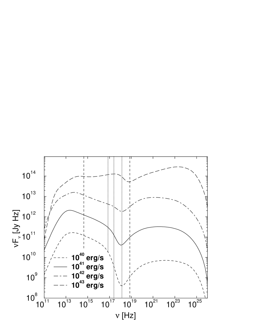
Figure 5: Time averaged photon spectra for different values of the flaring injection power $L_{\rm inj}^{\rm fl}$, from simulations no. 1, 2, 3, and 8. The dotted vertical lines indicate the frequencies at which light curves and hardness-intensity correlations have been extracted; the dashed vertical lines indicate the remaining two frequencies at which light curves have been extracted.

Figure 6: Optical and X-ray light curves for different values of the flaring injection power $L_{\rm inj}^{\rm fl}$, from simulations no. 1, 2, and 3.

Figure 7: Tracks in the harness-intensity diagrams at X-ray energies for different values of the flaring injection power $L_{\rm inj}^{\rm fl}$, from simulations no. 1, 2, 3, and 8. Symbols are the same as in Fig. 5: short-dashed ($10^{40}$ erg/s), solid ($10^{41}$ erg/s), dot-dashed ($10^{42}$ erg/s), long-dashed ($10^{43}$ erg/s). Stars indicate the locations at multiples of the dynamical time scale during the respective simulations.

Figure 8: Time averaged photon spectra for different intensities of the external soft radiation field, parametrized through different values of $\tau_{\rm T,BLR}$, from simulations no. 2, 5, 6, 7, and 18. The short-dashed curve shows a test simulation with constant magnetic field, while all other parameters were identical to the $\tau_{\rm T,BLR}=1$ simulation, illustrating the effect of our magnetic field parametrization as a constant fraction of the equipartition magnetic field. The dotted vertical lines indicate the frequencies at which light curves and hardness-intensity correlations have been extracted; the dashed vertical lines indicate the remaining two frequencies at which light curves have been extracted.

Figure 9: Optical and X-ray light curves for different intensities of the external soft radiation field, parametrized through different values of $\tau_{\rm T,BLR}$, from simulations no. 2, 6, and 7.

Figure 10: Tracks in the harness-intensity diagrams at X-ray energies for different intensities of the external soft radiation field, parametrized through different values of $\tau_{\rm T,BLR}$, from simulations no. 2, 6, and 7: solid ($\tau_{\rm T,BLR}=0$), dashed ($\tau_{\rm T,BLR}=0.1$), dot-dashed ($\tau_{\rm T,BLR}=1$). Stars indicate the locations at multiples of the dynamical time scale during the respective simulations.

Figure 11: Time averaged photon spectra for different values of the electron injection spectral index $q$, from simulations no. 2, 9, and 10. The dotted vertical lines indicate the frequencies at which light curves and hardness-intensity correlations have been extracted; the dashed vertical lines indicate the remaining two frequencies at which light curves have been extracted.

Figure 12: Optical and X-ray light curves for different values of the electron injection spectral indes $q$, from simulations no. 2, 9, and 10.

Figure 13: Tracks in the harness-intensity diagrams at X-ray energies for different values of the electron injection spectral index $q$, from simulations no. 2, 9, and 10: dashed ($q=2.2$), solid ($q=2.5$), dot-dashed ($q=2.8$). Stars indicate the locations at multiples of the dynamical time scale during the respective simulations.

Figure 14: Optical and X-ray light curves for different values of the duration of the flaring injection time scale, keeping the total energy input during the injection event constant (simulations no. 2, 11, and 12).

Figure 15: Tracks in the harness-intensity diagrams at X-ray energies for different values of the flaring injection time scale, keeping the total energy input during the injection event constant (simulations no. 2, 11, and 12): solid ($t_{\rm inj}=2\,t_{\rm dyn}$), dashed ($t_{\rm inj}=4\,t_{\rm dyn}$), dot-dashed ($t_{\rm inj}=6\,t_{\rm dyn}$). Stars indicate the locations at multiples of the dynamical time scale during the respective simulations.

Figure 16: Optical and X-ray light curves for different time profiles of the electron injection power, keeping the total energy input during the injection event constant (simulations no. 2, 14, and 15). The small insets illustrate the injection time profiles ($L_{\rm inj}$ vs. time).

Figure 17: Tracks in the harness-intensity diagrams at X-ray energies for different time profiles of the electron injection power, keeping the total energy input during the injection event constant (simulations no. 2, 14, and 15): solid (profile a = step function), dashed (profile c = triangular profile with $t_{r}=2\,t_{\rm dyn}$ and $t_{d}=0$), dot-dashed (profile d = triangular profile with $t_{r}=0$ and $t_{d}=2\,t_{\rm dyn}$). Stars indicate the locations at multiples of the dynamical time scale during the respective simulations.

Table 1: Parameters of the simulations used for our parameter study. Throughout the series of simulations, we have used $L_{\rm inj}^{\rm qu}=10^{38}$ ergs s^-1 (electron injection luminosity during quiescence), $\gamma_{1}=10^{3}$ (low-energy cutoff of injected electron spectrum), $\gamma_{2}=10^{5}$ (high-energy cutoff of injected electron spectrum), $D=10$ (Doppler boosting factor), $R_{b}=10^{16}$ cm (blob radius), and $\epsilon_{B}=1$ (magnetic-field equipartition parameter). The time profiles in the 6th column are: (a) step function, (b) triangular with linear rise and decay with equal time scales ($t_{\rm r,d}=t_{\rm inj}/2$), (c) linear rise and instantaneous drop ($t_{\rm r}=t_{\rm inj}$), (d) instantaneous rise and linear decay ($t_{\rm d}=t_{\rm inj}$). For time profiles (b) – (d), the parameter $L_{\rm inj}^{\rm fl}$ is the maximum injection power. $\eta$ is the electron escape time parameter, defined by $t_{\rm e,esc}=\eta\,R_{b}/c$. The parameters changed with respect to the base model (no. 2) printed in boldface.

Run no.	$L_{\rm inj}^{\rm fl}$ [ergs s-1]	$\tau_{\rm T,BLR}$	$q$	$\Delta t_{\rm inj}$	inj. time profile	$\eta$
1	1040	0	2.5	$2\,t_{\rm dyn}$	a	10
2	$10^{41}$	0	2.5	$2\,t_{\rm dyn}$	a	10
3	1042	0	2.5	$2\,t_{\rm dyn}$	a	10
4	$10^{41}$	10-3	2.5	$2\,t_{\rm dyn}$	a	10
5	$10^{41}$	10-2	2.5	$2\,t_{\rm dyn}$	a	10
6	$10^{41}$	10-1	2.5	$2\,t_{\rm dyn}$	a	10
7	$10^{41}$	1	2.5	$2\,t_{\rm dyn}$	a	10
8	1043	0	2.5	$2\,t_{\rm dyn}$	a	10
9	$10^{41}$	0	2.2	$2\,t_{\rm dyn}$	a	10
10	$10^{41}$	0	2.8	$2\,t_{\rm dyn}$	a	10
11	${\bf 5\times 10}^{\bf 40}$	0	2.5	4 tdyn	a	10
12	${\bf 3.33\times 10}^{\bf 40}$	0	2.5	6 tdyn	a	10
13	$2\times 10^{41}$	0	2.5	$2\,t_{\rm dyn}$	b	10
14	$2\times 10^{41}$	0	2.5	$2\,t_{\rm dyn}$	c	10
15	$2\times 10^{41}$	0	2.5	$2\,t_{\rm dyn}$	d	10
16	$10^{41}$	0	2.5	$2\,t_{\rm dyn}$	a	3
17	$10^{41}$	0	2.5	$2\,t_{\rm dyn}$	a	30
18∗	$10^{41}$	1	2.5	$2\,t_{\rm dyn}$	a	10

References

- Arbeiter, Pohl, & Schlickeiser (2002) Arbeiter, C., Pohl, M., & Schlickeiser, R., 2002, A&A, 386, 415
- Bednarek (1998) Bednarek, W., 1998, A&A, 336, 123
- Blandford & Levinson (1995) Blandford, R. D., & Levinson, A. 1995, ApJ, 441, 79
- Blaejowski et al. (2000) Blaejowski, M., Sikora, M., Moderski, R., & Madejski, G. M., 2000, ApJ, 545, 107
- Bloom & Marscher (1996) Bloom, S. D., & Marscher, A. P., 1996, ApJ, 461, 657
- Böttcher (2002) Böttcher, M., 2002, in proc. of “The Gamma-Ray Universe”, XXII Moriond Astrophysics Meeting
- Böttcher et al. (2002) Böttcher, M., Aller, H. D., Aller, M. F, Mang, O., Raiteri, C. M., Ravasio, M., Tagliaferri, G., Teräsranta, H., & Villata, M., 2002, in proc. “Blazar Astrophysics with BeppoSAX and other Observatories”, special ASI public., Eds. P. Giommi, E. Massaro, & G. Palumbo, in press
- Böttcher & Bloom (2000) Böttcher, M., & Bloom, S. D., 2000, AJ, 119, 469
- Böttcher & Dermer (1998) Böttcher, M., & Dermer, C. D., 1998, ApJ, 501, L51
- Böttcher & Dermer (2002) Böttcher, M., & Dermer, C. D., 2002, ApJ, 564, 86
- Böttcher, Mause, & Schlickeiser (1997) Böttcher, M., Mause, H., & Schlickeiser, R., 1997, A&A, 324, 395
- Böttcher, Mukherjee, & Reimer (2002) Böttcher, M., Mukherjee, R., & Reimer, A., 2002, ApJ, 581, in press
- Böttcher & Schlickeiser (1997) Böttcher, M., & Schlickeiser, R., 1997, A&A, 325, 866
- Buckley (2001) Buckley, J. H., in proc. of “Gamma 2001”, Eds. S. Ritz, N. Gehrels, & C. R. Shrader, AIP Conf. Proc. 587, p. 235
- Cavaliere & D’Elia (2002) Cavaliere, A., & D’Elia, V., 2002, ApJ, 571, 226
- Chiaberge & Ghisellini (1999) Chiaberge, M., & Ghisellini, G., 1999, MNRAS, 306, 551
- Chiang & Böttcher (2002) Chiang, J., & Böttcher, M., 2002, ApJ, 564, 92
- Chiapetti et al. (1999) Chiappetti, L., et al., 1999, ApJ, 521, 552
- Costamante & Ghisellini (2002) Costamante, L., & Ghisellini, G., 2002, A&A, 384, 56
- de Jager & Stecker (2002) de Jager, O., & Stecker, F. W., 2002, ApJ, 566, 738
- D’Elia & Cavaliere (2000) D’Elia, V., & Cavaliere, A., 2000, PASP, 227, 252
- Dermer & Schlickeiser (1993) Dermer, C. D., & Schlickeiser, R., 1993, ApJ, 416, 458
- Dermer & Schlickeiser (2002) Dermer, C. D., & Schlickeiser, R., 2002, ApJ, in press
- Dermer, Schlickeiser, & Mastichiadis (1992) Dermer, C. D., Schlickeiser, R., & Mastichiadis, A., 1992, A&A, 256, L27
- Dermer, Sturner, & Schlickeiser (1997) Dermer, C. D., Sturner, S. J., & Schlickeiser, R., ApJS, 109, 103
- Edelson et al. (2001) Edelson, R., Griffiths, G., Markowitz, A., Sembay, S., Turner, M. J. L., & Warwick, R., 2001, ApJ, 554, 274
- Fossati et al. (1998) Fossati, G., Maraschi, L., Celotti, A., Comastri, A., & Ghisellini, G., 1998, MNRAS, 299, 433
- Fossati et al. (2000) Fossati, G., et al., 2000, ApJ, 541, 153
- Gaidos et al. (1996) Gaidos, J. A., et al., 1996, Nature, 383, 319
- Georganopoulos & Marscher (1998) Georganopoulos, M., & Marscher, A. P., 1998, ApJ, 506, L11
- Ghisellini et al. (1998) Ghisellini, G., Celotti, A., Fossati, G., Maraschi, L., & Comastri, A., 1998, MNRAS, 301, 451
- Ghisellini & Madau (1996) Ghisellini, G., & Madau, P., 1996, MNRAS 280, 67
- Hartman et al. (1999) Hartman, R. C., et al., 1999, ApJS, 123, 79
- Hartman et al. (2001) Hartman, R. C., et al., 2001, ApJ, 553, 683
- Kataoka et al. (2000) Kataoka, J., Takahashi, T., Makino, F., Inoue, S., Madejski, G. M., Tashiro, M., Urry, C. M., & Kubo, H., 2000, ApJ, 528, 243
- Kirk, Rieger, & Mastichiadis (1998) Kirk, J. G., Rieger, F. M., & Mastichiadis, A., 1998, A&A, 333, 452
- Krawczynski, Coppi, & Aharonian (2002) Krawczynski, H., Coppi, P. S., & Aharonian, F. A., 2002, MNRAS, in press
- Kusunose, Takahara, & Li (2000) Kusunose, M., Takahara, F., & Li, H., 2000, ApJ, 536, 299
- Li & Kusunose (2000) Li, H., & Kusunose, M., 2000, ApJ, 536, 729
- Madejski (1998) Madejski, G., 1998, in “Theory of Black Hole Accretion Disks”, Eds. M. Abramowicz, G. Bjørnsson, & J. Pringle (Cambridge University Press), p. 21
- Madejski et al. (1999) Madejski, G., et al., 1999, ApJ, 521, 145
- Maraschi, Ghisellini, & Celotti (1992) Maraschi, L., Ghisellini, G., & Celotti, A., 1992, ApJ, 397, L5
- Marscher & Gear (1985) Marscher, A. P., & Gear, W. K., 1985, ApJ, 298, 114
- Moderski, Blaejowski, & Sikora (2002) Moderski, R., Blaejowski, M., & Sikora, M., 2002, A&A, submitted
- Mukherjee et al. (1997) Mukherjee, R., et al., 1997, ApJ, 490, 116
- Padovani & Urry (2001) Padovani, P., & Urry, C. M., 2001, in proc. of “Blazar Demographics and Physics”, ASP Conf. Series, eds. P. Padovani, & C. M. Urry, in press
- Press et al. (1992) Press, W. H., Teukolsky, S. A., Vetterling, W. T., & Flannery, B. P., 1992, “Numerical Recipes in C”, Cambridge University Press
- Rachen (2000) Rachen, J., 2000, AIP Conf. Proc., 515, 41
- Ravasio et al. (2002) Ravasio, M., et al., 2002, A&A, 383, 763
- Sambruna (2000) Sambruna, R. M., 2000, AIP Conf. Proc., 515, 19
- Sambruna, Maraschi, & Urry (1996) Sambruna, R. M., Maraschi, L., & Urry, C. M., 1996, ApJ, 463, 444
- Sembay et al. (2002) Sembay, S., Edelson, R., Markowitz, A., Griffiths, R. G., & Turner, M. J. L., 2002, ApJ, submitted (astro-ph/0204179)
- Sikora, Begelman, & Rees (1994) Sikora, M., Begelman, M. C., & Rees, M. J., 1994, ApJ, 421, 153
- Sikora et al. (2001) Sikora, M., Blaejowski, M., Begelman, M. C., & Moderski, R., 2001, ApJ, 554, 1; Erratum: ApJ, 561, 1154 (2001)
- Tagliaferri et al. (2000) Tagliaferri, G., et al., 2000, A&A, 354, 431
- Takahashi et al. (1996) Takahashi, T., et al., 1996, ApJ, 470, L89
- Takahashi et al. (2000) Takahashi, T., et al., 2000, ApJ, 542, L105
- Tavecchio, Maraschi, & Ghisellini (1998) Tavecchio, F., Maraschi, L., & Ghisellini, G., 1998, ApJ, 509, 608
- Urry & Padovani (1995) Urry, C. M., & Padovani, P., 1995, PASP, 107, 803
- von Montigny et al. (1995) von Montigny, C., et al., 1995, ApJ, 440, 525
- Zheng et al. (1999) Zheng, Y., et al., 1999, ApJ, 527, 719