Elemental Abundances and Ionization States within the Local Interstellar Cloud Derived from HST and FUSE Observations of the Capella Line of Sight11affiliation: Based on observations made with the NASA-CNES-CSA Far Ultraviolet Spectroscopic Explorer. FUSE is operated for NASA by the Johns Hopkins University under NASA contract NAS5-32985. Also based on observations with the NASA/ESA Hubble Space Telescope, obtained from the Data Archive at the Space Telescope Science Institute, which is operated by the Association of Universities for Research in Astronomy, Inc., under NASA contract NAS5-26555.
Abstract
We use ultraviolet spectra of Capella from the Hubble Space Telescope (HST) and Far Ultraviolet Spectroscopic Explorer (FUSE) satellites to study interstellar absorption lines from the Local Interstellar Cloud (LIC). Measurements of these lines are used to empirically determine the ionization states of carbon, nitrogen, and silicon in the LIC, for comparison with the predictions of theoretical photoionization models. We find that the observed ionization states are consistent with previously published photoionization predictions. Total abundances are determined for the elements mentioned above, and others, for comparison with solar abundances. Magnesium, aluminum, silicon, and iron are all depleted by at least a factor of 10 toward Capella. The abundances of carbon, nitrogen, and oxygen are essentially solar, although the error bars are large enough to also allow depletions of about a factor of 2 for these elements.
1 INTRODUCTION
The Sun is located inside a warm, partially ionized interstellar cloud called the Local Interstellar Cloud (LIC). Ultraviolet spectra containing LIC absorption lines have been used to study the properties of the LIC. Its average temperature appears to be about K, although there is some evidence for spatial variation within the LIC (Linsky et al., 1995; Dring et al., 1997; Piskunov et al., 1997; Wood & Linsky, 1998; Wood, Redfield, & Linsky, 2002a). The average H I density is cm-3 (Linsky et al., 2000). Hydrogen must be roughly half-ionized since the average electron density is cm-3 (Wood & Linsky, 1997; Holberg et al., 1999). Estimates of from observations of interstellar atoms passing through the heliosphere suggest somewhat higher H I densities of cm-3 (Quémerais et al., 1994; Izmodenov et al., 1999), possibly suggesting the presence of density and/or hydrogen ionization state variations within the LIC. Ionization state variations are to be expected since different parts of the LIC will be shielded from photoionization sources to different extents (Bruhweiler & Cheng, 1988; Cheng & Bruhweiler, 1990; Slavin & Frisch, 2002). Measurements of interstellar material flowing through the heliosphere and local interstellar medium (LISM) absorption line studies all suggest that in a heliocentric rest frame the LIC appears to be flowing towards Galactic coordinates and , with a speed of about 25.7 km s-1 (Witte et al., 1993; Witte, Banaszkewicz, & Rosenbauer, 1996; Lallement & Bertin, 1992; Lallement et al., 1995; Quémerais et al., 2000).
Probably the best line of sight for studying absorption by gas in the LIC is that toward Capella, which is a spectroscopic binary system (G8 III+G1 III) located 12.9 pc away, with Galactic coordinates and . There are several reasons why this line of sight is ideal. First of all, there is only one interstellar velocity component observed for this short line of sight, that of the LIC. Short lines of sight are preferable for studying the LIC to avoid a complicated, multi-component ISM structure that is often difficult to resolve into individual components. Secondly, although cool stars are not as bright in the UV as hot stars, Capella is the brightest cool star in the sky in the ultraviolet, providing sufficient background in the continuum and bright emission lines to observe numerous LIC absorption lines. There are few nearby hot stars (including hot white dwarfs) that can be observed for LIC studies, which means one must generally observe cool stars like Capella. The UV emission lines from the Capella stars are quite broad, making it easy to distinguish narrow ISM lines located within the broad emission profiles, which serve as the continuum for measuring the ISM lines.
Another advantage of the Capella line of sight is that LIC column densities are particularly high in this direction, allowing us to detect weak absorption lines that would be undetectable in other directions. This is illustrated by Figure 1, a schematic picture of the structure of the LISM in the Galactic plane, showing that the Capella line of sight passes through the entire length of the LIC. The LIC outline in Figure 1 is from the model of Redfield & Linsky (2000). The shape of the nearby “G cloud” is a crude estimate from Wood, Linsky, & Zank (2000), and there is some question as to whether this cloud is truly distinct from the LIC (see Wood et al., 2002a). Also shown is an equally crude estimate of the shape of a cloud detected toward Sirius (dotted line), which might be the same cloud as the “Hyades Cloud” identified by Redfield & Linsky (2001) in the direction of the Hyades Cluster. The lines of sight to the stars shown in Figure 1 have all been studied by the Hubble Space Telescope (HST) to better understand the properties of the LISM. Since all the stars are from the Galactic plane, distortions due to the projection effects in showing the three-dimensional LISM as a two-dimensional figure are not severe. The direction toward the B2 II star CMa is indicated in Figure 1. This star is important because it is the dominant stellar source of ionizing photons irradiating the LIC (Vallerga & Welsh, 1995).
Several studies of the Capella line of sight have been published using data from the Goddard High Resolution Spectrograph (GHRS) formerly aboard HST. Linsky et al. (1993, 1995) analyzed LIC absorption lines of H I, D I, Mg II, and Fe II toward Capella, with the primary goal being to measure the D/H ratio within the LIC. Vidal-Madjar et al. (1998) also analyzed the HST/GHRS data and found close agreement with the results of Linsky et al. (1993, 1995), although Vidal-Madjar & Ferlet (2002) claim that the analysis of H I should have larger uncertainties due to the possible existence of undetected hot H I absorption components. Wood & Linsky (1997) measured the electron density toward Capella using observations of C II 1334.5 and C II∗ 1335.7.
One problem with the GHRS instrument is that its one dimensional detector could only observe a relatively narrow wavelength region for each exposure. However, in 1997 the GHRS was replaced with the Space Telescope Imaging Spectrograph (STIS). The STIS instrument has capabilities similar to the GHRS in terms of spectral resolution and sensitivity, but it has a two-dimensional detector providing much broader wavelength coverage for each observation. On 1999 September 12, HST/STIS observed the Å spectrum of Capella using the E140M grating. This observation provides access to many LIC absorption lines unavailable in the GHRS data set. The Far Ultraviolet Spectroscopic Explorer (FUSE) has also observed Capella recently. The FUSE satellite obtains spectra at wavelengths shorter than those accessible to HST, from Å, allowing access to still more ISM absorption features.
In this paper, we use the new FUSE and HST/STIS data to provide a complete analysis of UV absorption lines detected towards Capella. Our primary goal is to measure column densities for as many atomic species as possible to establish the ionization states and abundances of various elements within the LIC.
2 OBSERVATIONS
Table 1 lists the HST/STIS and FUSE observations of Capella analyzed in this paper. The STIS instrument is described in detail by Kimble et al. (1998) and Woodgate et al. (1998). The stellar Fe XXI 1354.1 emission line in the STIS spectrum was analyzed by Johnson et al. (2002), and the stellar emission lines in the FUSE data were studied by Young et al. (2001). Here we are obviously interested in the LIC absorption lines present in these data. The HST/STIS data obtained on 1999 September 12 were processed using the IDL-based CALSTIS software package (Lindler, 1999). This processing includes an accurate wavelength calibration using an exposure of the onboard wavelength calibration lamp obtained contemporaneous with the Capella exposures, and a correction for scattered light within the spectrograph.
On 2000 November 5, FUSE observed Capella through the low resolution (LWRS) aperture. The observation consisted of 10 separate exposures adding up to a total exposure time of 14,182 s. A nearly identical 10-exposure observation of Capella was obtained two days later on 2000 November 7 with a total exposure time of 12,332 s. A third observation of Capella was made through the medium resolution (MDRS) aperture on 2001 January 11, consisting of 28 separate exposures totaling 21,359 s. These data were reduced with version 1.8.7 of the CALFUSE pipeline software, although for the H I Ly spectral region, we found it necessary to use spectra processed using the more recent CALFUSE 2.0.5 version (see §3.4).
Given Capella’s orbital period of 104 days, the two LWRS observations were made close enough in time (and therefore orbital phase) that we can coadd the two data sets to produce a single LWRS spectrum. However, the MDRS data must be kept separate, because this data set was obtained with the Capella binary at orbital phase (near opposition), while the LWRS data were obtained at (closer to quadrature). Thus, the centroids of the emission lines from the two Capella stars are different for the two data sets, changing the composite line profiles. The spectra must therefore be analyzed separately. Another reason for keeping the data separate involves airglow emission. The large size of the LWRS aperture means that H I and O I airglow emission features from the Earth’s geocorona are very prominent in the LWRS spectrum, whereas the airglow features are greatly suppressed in the MDRS data due to the much smaller size of the MDRS aperture. Because of the reduced airglow, there are H I, D I, and O I absorption features visible in the MDRS data that are largely or completely obscured in the LWRS data. The existence of the separate MDRS data set therefore allows us to analyze absorption lines that are not visible in the LWRS data.
In order to fully cover its 905–1187 Å spectral range, FUSE has a multi-channel design — two channels (LiF1 and LiF2) use Al+LiF coatings, two channels (SiC1 and SiC2) use SiC coatings, and there are two different detectors (A and B). For a full description of the instrument, see Moos et al. (2000). With this design FUSE acquires spectra in 8 segments (LiF1A, LiF1B, LiF2A, LiF2B, SiC1A, SiC1B, SiC2A, and SiC2B) covering different, overlapping wavelength ranges. We cross-correlated and coadded the individual FUSE exposures to create a single LWRS and MDRS spectrum for each segment. We decided not to coadd the individual segments to ensure that such an operation would not degrade the spectral resolution.
Since there is no wavelength calibration lamp onboard FUSE, the wavelength scale produced by the FUSE data reduction pipeline is very uncertain. Fortunately, there are two strong, narrow interstellar absorption lines in the Capella spectrum that can be used to fix the wavelength scale for all of the segments except LiF2A and LiF1B (see Redfield et al., 2002). These lines are C III 977.0 and C II 1036.3. As mentioned in §1, the Capella line of sight has only one interstellar velocity component, which is identified with the LIC and centered at a heliocentric velocity of km s-1 (Linsky et al., 1993, 1995). By shifting each spectral segment so that the ISM absorption is centered at this velocity, we can calibrate the wavelength scales to within km s-1.
3 FITTING THE LIC ABSORPTION LINES
3.1 Carbon, Nitrogen, and Silicon
Our goal is to measure LIC column densities for as many atomic species as possible using the full HST and FUSE data sets. We searched the spectra for absorption lines using the Morton (1991) line list. Our initial attention focused on lines of carbon, nitrogen, and silicon, because for the lowest three ionization states of these elements we can either measure a column density from detected absorption lines or measure a meaningful upper limit from undetected lines. Figure 2 shows the detected and undetected lines that we use to measure these column densities. Note that there are 3 N I and 3 Si II lines used to measure the N I and Si II columns. We use the undetected C I 1656.9, N III 989.8, Si I 1562.0, and Si III 1206.5 lines to estimate upper limits for those species. The C II 1334.5 line in Figure 2 is not from our STIS data, but is from a GHRS spectrum that has higher spectral resolution than the STIS data analyzed here. Since the GHRS C II line was previously analyzed by Wood & Linsky (1997), it is not analyzed again here, but we reproduce the C II profile and fit in Figure 2 for the sake of completeness.
Fits to the detected LIC absorption lines are shown in Figure 2. Polynomial fits to the wavelength regions surrounding the absorption lines are used to estimate the continuum above each line. Best fits to the lines are determined by a minimization routine. Dotted lines show the fits before convolution with the instrumental line spread function (LSF), and thick solid lines show the fits after convolution with the LSF, which fit the data. For the STIS data, we use the appropriate LSF from Sahu et al. (1999). The FUSE LSF is unfortunately not very well known. Furthermore, it is wavelength dependent and quite possibly changes from one observation to the next (see, e.g., Kruk et al., 2002). We use the average FUSE LSF derived by Wood et al. (2002b) from the analysis of white dwarf spectra, recognizing that this profile will only apply to our data in an approximate sense. However, since we typically assume Doppler broadening parameters rather than try to derive them from the fits (see below), we do not believe that inaccuracies in the LSF will result in significant errors in our results. The three N I lines in Figure 2 are fitted simultaneously to measure the N I column density, as are the three Si II lines to derive the Si II column.
None of the detected absorption lines are fully resolved in either the STIS or the FUSE spectra. Based on the analysis of higher resolution GHRS observations of fully resolved H I, D I, Mg II, and Fe II lines, Linsky et al. (1993, 1995) measured a temperature and nonthermal velocity for the LIC toward Capella of K and km s-1, respectively. (The errors include both random and systematic errors combined linearly). We can use these measurements to constrain the Doppler broadening parameters () of our lines using the relation
| (1) |
where is the atomic weight of the element in question and is in units of km s-1. As an example, for N lines () the Doppler parameter can be constrained to be in the range km s-1. By constraining the Doppler parameters in this way, we can obtain more precise column density measurements from the unresolved spectral lines. For the N I and Si II lines, we tried relaxing this constraint since we had several lines of differing strengths to work with (see Figure 2), which collectively provide constraints for even though the lines are not resolved. We did not obtain results significantly different from the fits in which the value of is constrained.
Table 2 provides a summary of all column density measurements for LIC absorption lines observed toward Capella. Some of the measurements are based on previous work, as indicated by the last column of the table. The column densities we measure here are also listed in the table. The new column densities quoted in Table 2 are actually the product of two independent analyses. Two of us (B. E. W. and S. R.) reduced and analyzed the STIS and FUSE data separately. Although the measurement techniques are essentially identical, as described above, the continuum placement will be different since it will depend on exactly how broad a region beyond the lines is fitted with the polynomial and what order of polynomial is used. The fact that the data are reduced independently in these analyses is also significant, especially for the FUSE data because the manner in which individual exposures are cross-correlated and coadded can lead to differences in the reduced spectrum. Thus, this exercise allows us to see if two important potential sources of systematic error are seriously affecting our results.
The independent measurements proved to be reasonably consistent in that the error bars of the measured column densities overlap nicely, suggesting that the dominant source of uncertainty is not continuum placement or data reduction, but is instead the uncertainty in the Doppler parameters, which arises from the uncertainties in and (see above). The independent measurements are certainly not identical, though, and the new column densities and uncertainties reported in Table 2 are averages of the two results. For example, for Si II the independent analyses suggest and , so the compromise value reported in Table 2 based on averaging is .
The lines in Figure 2 that come from FUSE spectra are C III 977.0, N II 1084.0, and N III 989.8. The data shown in the figure are the LWRS data, but we also fit the MDRS data, and our derived column densities are compromises between the two separate fits. In Table 2, we list the segment used in the analysis of the FUSE lines, although we check all segments for consistency. For the C III and N III lines, we choose the SiC2A segment, as the SiC1B segment that also contains these lines is noisier and has significantly lower spectral resolution than SiC2A. For N II, we use the SiC2B segment. Figure 3 compares the N II line seen by SiC2B with the SiC1A segment that also contains this line, for both the LWRS and MDRS data. For some reason the LIC absorption feature is not seen in the SiC1A MDRS data, but its detection in the other three cases leads us to conclude that the detection is valid and that the MDRS SiC1A spectrum is misleading. It is known that FUSE’s spectral resolution can decrease near the ends of segments. Thus, perhaps the resolution of SiC1A degrades enough at the location of the N II line to make detection impossible, at least for the MDRS spectrum, thereby forcing us to base our measurements on the SiC2B data.
The uncertainties reported in Table 2 should be considered to be roughly 2 uncertainties, although the issue is not free from ambiguity. For the new measurements presented in this paper, we always assume values based on the and measurements and their uncertainties from Linsky et al. (1995). The random error contributions to the and uncertainties reported by Linsky et al. (1995) are 2, but it is difficult to know what confidence level to assign to the systematic error contributions that they estimate. By adding the two linearly rather than in quadrature we hope we are being conservative enough to still consider the final total errors in and (i.e., K and km s-1) to be , meaning the column density errors in this paper reported in this paper should also be . The H I column in Table 2 is from Linsky et al. (1995), but we assign a larger uncertainty to this quantity based on the results of Vidal-Madjar & Ferlet (2002) concerning possible systematic errors involved in the analysis. As is often the case for systematic errors, the exact confidence level to associate with this uncertainty is unclear.
3.2 Oxygen
The O I lines available for analysis are shown in Figure 4. The O I 1302.2 line observed by STIS has excellent S/N but is the most highly saturated of the three lines. The O I 988.7, 988.8, and 1039.2 lines observed by FUSE are covered by airglow emission in the LWRS spectra, so we can only use the MDRS data.
Table 2 lists the segments used for the FUSE lines. The 1039.2 line in Figure 4 is from the LiF1A channel. The SiC1A and SiC2B segments that also contain this line are too noisy to be of any use, simply due to the lower sensitivity of the SiC detectors. The absorption feature is also not clearly detected in the LiF2B channel, but the reason for this is unclear. Nevertheless, we still consider the LiF1A detection solid, because the absorption must be present in the line at about the level seen in Figure 4 based on the strength of the O I absorption in the other lines shown in the figure.
We fit the O I lines separately, except for the adjacent 988.7 and 988.8 lines, constraining the Doppler parameter as described in §3.1. The best fits are shown in Figure 4, and the column densities are listed in Table 2. The weighted mean of these three values for is 15.02. We cannot use a standard deviation for our error bar, because the uncertainties of the three measurements are correlated through the assumed range of values. Thus, we simply use the smallest of the three uncertainties, 0.32 dex, as our error estimate, resulting in a final value of . This is consistent with the estimate of Linsky et al. (1995) based on a lower quality HST/GHRS observation of the O I 1302.2 line.
3.3 Other Metal Lines
There is only one other metal line that is detected in the data, Al II 1670.8. This line and our best fit to it is shown in Figure 5, and the column density [] is listed in Table 2. The km s-1 velocity of the Al II line agrees reasonably well with the previously measured LIC velocity toward Capella of km s-1 (Linsky et al., 1995), which helps convince us that this weak LIC line is real. Besides the C, N, and Si lines discussed in §3.1, we also list in Table 2 upper limits for column densities of a few other metal lines that are potentially useful: C IV 1548.2, S II 1259.5, and Ar I 1048.2.
3.4 Hydrogen and Deuterium
The H I and D I column densities toward Capella have previously been measured using HST/GHRS observations of the Ly line (Linsky et al., 1993, 1995). The more recent FUSE data allow access to the higher lines of the Lyman series, although we must confine our attention to the MDRS data since the LWRS data are contaminated with strong airglow emission. There is D I absorption detected in the Ly line at 1025.7 Å, and initially we hoped to analyze the Ly line to test the results of the HST Ly analysis. This proved impossible, however, partly due to problems with the FUSE “walk correction” (see below). Nevertheless, the D I detection and the data reduction difficulties for Ly might be instructive and of some interest to the reader, so we now describe the data and our problems with reducing and analyzing it in more detail.
The solid line in Figure 6 shows the LiF1A Ly profile that is produced by processing the FUSE MDRS data through CALFUSE 1.8.7. Vertical lines in the figure show where we expect the centroids of the D I and H I absorption to be located. There is an absorption feature at about 1025.6 Å that looks like it could be D I absorption, but it is redshifted from where it should be by Å ( km s-1), while the interstellar H I absorption feature is roughly centered correctly. The problem can be traced to a detector effect where the recorded position of each photon event is a slight function of the pulse height of the event, which we now describe in more detail.
Each incident photon creates a cascade of electrons at the back of the FUSE microchannel plate detectors. When these electrons are read out by the detector, the position of the event is recorded by the detector electronics. Unfortunately, the accuracy of this determination is degraded for low pulse height events (i.e., events creating a weaker shower of electrons). This variation of position with pulse height is known as the walk. Furthermore, the FUSE detectors are gradually losing sensitivity as they are continually exposed to more photons. This “gain sag” means a significant increase in low pulse height events and inaccuracies in the wavelength positions of the detected photons (Sahnow et al., 2000). This problem is most severe at the location of Ly, because the detector is constantly exposed to substantial H I Ly airglow emission. This is particularly true for LWRS data, but Figure 6 shows that it can be a problem for MDRS data as well. The gain sag that leads to the walk problem can be mitigated by increasing the voltage of the FUSE detectors, thereby increasing the gain. So far, this has been done twice since launch. Unfortunately, the first increase on 2001 January 24 happened just a couple weeks after the MDRS observation of Capella, meaning the gain sag had reached about its worst point at the time of the Capella observation and has since been improved.
Further calibration efforts by the FUSE instrument team have led to a software correction for the walk problem, which is included in the more recent version of the pipeline software, CALFUSE 2.0.5. The Capella data were obtained in TIME-TAG mode, where the individual pulse height events associated with each detected photon are recorded and stored. Thus, we can reprocess the data with the walk correction included to try to more accurately assign wavelengths for each event. The dotted line in Figure 6 shows the LiF1A profile of Ly that results from data processing through CALFUSE 2.0.5. The improved data reduction shifts the D I absorption to roughly the correct location. Note that it also broadens the H I absorption.
In Figure 7, we show the Ly line from all four FUSE segments that contain the line, after processing with CALFUSE 2.0.5. Also shown are estimates of the intrinsic stellar profile, and predictions for what the D I and H I absorption should look like based on the H I and D I column densities measured from Ly (Linsky et al., 1995). There are some subtle differences in the Ly profile as seen by the various FUSE segments, particularly in the neighborhood of D I. These differences lead to slight differences in the shapes of the stellar Ly profile estimated for each segment. The D I absorption seems stronger and more clearly detected in the noisier SiC segments. While D I in the CALFUSE 1.8.7 spectrum in Figure 6 was highly redshifted, it now seems to be slightly blueshifted in the CALFUSE 2.0.5 spectra. All these issues may be indications of residual difficulties with the walk problem. In any case, we do not believe the FUSE Ly data to be of high enough quality to improve upon the HST Ly results, but Figure 7 shows that the D I and H I Ly absorption is observed to be at least roughly consistent with the HST Ly analysis.
4 THE IONIZATION STATES OF C, N, AND Si WITHIN THE LIC
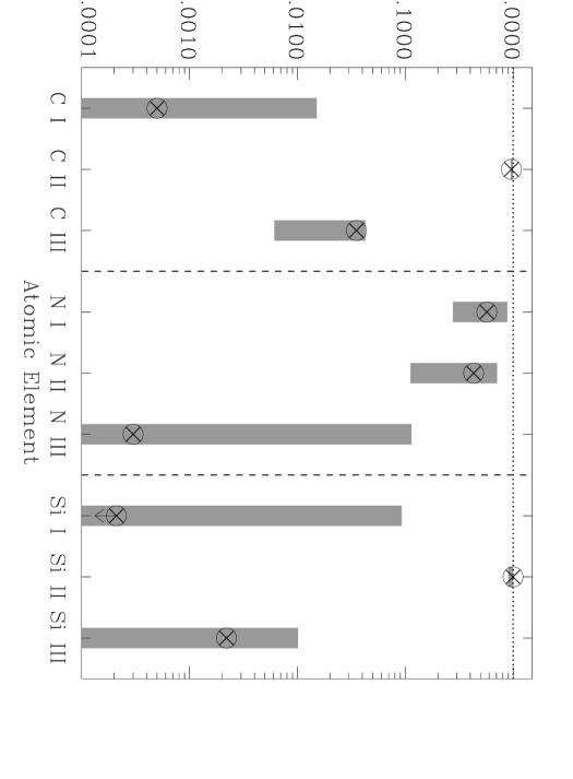
The column density measurements and upper limits in Table 2 include measurements for the three lowest ionization states of C, N, and Si. Based on these measurements, we can compute the ionization fractions for these elements within the LIC. Because upper limits are involved (for C I, N III, Si I, and Si III), we cannot quote a best value and an error for the ionization fractions, so instead we compute ionization fraction ranges allowed by the measurements. These ranges are listed in Table 3 and are also displayed graphically in Figure 8. At least 95% of carbon is in the form of C II. Nitrogen is divided roughly equally between N I and N II, although uncertainties are high due to the imprecise N II measurement. At least 90% of silicon is Si II. Since the doubly ionized species (C III, N III, and Si III) have only trace abundances, we are confident that higher ionization states are even more insignificant, and we note that there is clearly no C IV 1548.2 or Si IV 1393.8 absorption toward Capella.
In Figure 8, we compare the ionization fraction ranges allowed by the Capella observations with the predictions of a photoionization model from Slavin & Frisch (2002, hereafter SF02), in particular their favored model 17. In their models, SF02 estimate the ionizing extreme ultraviolet (EUV) radiation field incident on the LIC based on the known stellar EUV sources, dominated by CMa (B2 II), and estimates for the more poorly known diffuse EUV background. Radiative transfer calculations are then used to compute ionization fractions at the solar location within the LIC. The comparison of these model predictions with our measurements in Figure 8 is only valid in an approximate sense, because our measurements are average values for the Capella line of sight rather than for the LIC material in the immediate vicinity of the Sun. Nevertheless, despite this difference Figure 8 shows that the observed ionization states of C, N, and Si toward Capella are consistent with the predictions of SF02.
The models of SF02 rely heavily on observations of LIC absorption towards CMa (Gry et al., 1995; Gry & Jenkins, 2001). Gry & Jenkins (2001) detect C IV and Si III absorption at the LIC velocity toward CMa, in contrast to our low upper limits for these species (see Table 2). Numerically, Gry & Jenkins (2001) find and . These results are inconsistent with our upper limits, and . The Si III discrepancy is particularly striking, and SF02 comment on the difficulty of explaining any substantial amount of Si III existing within the LIC, although the low C IV column could possibly be explained as absorption from a conductive interface with the hot ISM. However, since we see no C IV and Si III absorption towards Capella it seems likely that the absorption seen toward CMa is not really from the LIC, but is instead from another component that happens to be at the LIC velocity along the long line of sight to CMa. This was also the conclusion of Hébrard et al. (1999), who noted that no Si III absorption is seen toward Sirius, a line of sight very near that of CMa but much shorter (see Fig. 1).
The agreement between the measured and predicted ionization states in Figure 8 supports the view that photoionization alone can account for the ionization state of the LIC. However, SF02 presented a total of 25 different photoionization models for the LIC, and all 25 are consistent with our observations, meaning our measurements are unfortunately not precise enough to be be used to test the assumptions behind the individual models. The size of the error bars in Figure 8 also means the test of the photoionization models is not as stringent as we would like, and in any case it remains possible that elements other than C, N, and Si are not in photoionization equilibrium. Jenkins et al. (2000) present another argument in favor of photoionization equilibrium within the LISM in general, pointing out that the low Ar I/H I ratios observed toward several nearby white dwarfs are consistent with expectations for photoionization, since Ar has a large photoionization cross section. Unfortunately, we were not able to detect the Ar I 1048.2 line toward Capella, and the upper limit in Table 2 is not very helpful.
An alternative to the steady state photoionization model is the possibility that the LIC is not in ionization equilibrium at all but was collisionally ionized in the distant past ( years ago) by a passing shock wave, perhaps from a supernova, and ionization equilibrium has still not been reestablished (Lyu & Bruhweiler, 1996). The high ionization state of He within the LISM, as determined from Extreme Ultraviolet Explorer (EUVE) measurements (Vennes et al., 1993; Holberg et al., 1995; Dupuis et al., 1995; Lanz et al., 1996), appears to support this view, since the known stellar EUV background certainly cannot ionize He to the observed extent (Vallerga, 1998). Further evidence for non-equilibrium conditions in the LISM is provided by Breitschwerdt (2001), who has suggested that observations of X-ray and EUV emission from the hot Local Bubble surrounding the LIC are more easily explained by non-equilibrium models.
For the LIC, the whole issue hinges on the nature of the diffuse EUV background. Unfortunately, the properties of this emission are poorly known. In their photoionization models, SF02 use a measurement of the soft X-ray background from sounding rockets (McCammon et al., 1983) and plasma models to infer the EUV background from the hot plasma within the Local Bubble. They also include another diffuse component based on theoretical estimates of radiation from evaporative boundaries of local clouds like the LIC. With this assumed background, SF02 can ionize He to the required degree, and their predictions for C, N, and Si are consistent with our results, as mentioned above. However, upper limits on the diffuse EUV background provided by the Extreme Ultraviolet Explorer (EUVE) satellite are lower than the SF02 estimate by a factor of (Jelinsky, Vallerga, & Edelstein, 1995). Fortunately, this issue should be resolved by the soon-to-be-launched Cosmic Hot Interstellar Plasma Spectrometer (CHIPS) satellite, which (unlike EUVE) is designed to measure diffuse EUV emission (Hurwitz & Sholl, 1999).
Once CHIPS provides a more definitive measurement of the diffuse EUV background, the whole issue of whether the LIC is in photoionization equilibrium or is out of equilibrium entirely should be revisited. For now, we regard the comparison of theoretical and observed ionization fractions in Figure 8 as providing some support for the accuracy of the photoionization models of SF02, at least for the elements with which we are concerned.
5 ELEMENTAL ABUNDANCES WITHIN THE LIC
We now estimate total gas-phase abundances for the elements for which we have column density measurements. Absolute abundances must be measured relative to the dominant element in the universe, hydrogen, so we must first estimate the total hydrogen column density toward Capella, including both H I and H II. The H I column has been measured from HST/GHRS observations of Ly. The H I column that we assume in Table 2 is from Linsky et al. (1995), but we assign a larger uncertainty to this quantity based on the results of Vidal-Madjar & Ferlet (2002). The H II column density toward Capella cannot be measured directly.
Wood & Linsky (1997) determined that the average electron density within the LIC toward Capella lies in the range cm-3 based on the column density ratio of C II 1334.5 and C II∗ 1335.7. Most of the electrons within the LIC will come from ionized hydrogen, but since He is ionized to nearly the same degree as hydrogen in the LISM (see §4), roughly 10% will come from He. Thus, we assume . This number density of H II can be converted to a column density only if we know the distance to the edge of the LIC toward Capella, . The highest average H I densities within the LIC toward the nearest stars are cm-3 (see, e.g., Linsky et al., 2000), but estimates of within the LIC based on measurements of interstellar H I within the heliosphere have suggested that could be more like 0.2 cm-3 (Quémerais et al., 1994; Izmodenov et al., 1999). Assuming cm-3, we find that pc based on the value in Table 2. We can then compute the H II column from . In this way, we estimate , and the H ionization fraction range implied by this value is listed in Table 3. The total hydrogen column (H I+H II) is then .
We can now compute elemental abundances relative to H from the column densities listed in Table 2. For each element, we add the columns of all detected ionization states. We use the ionization state calculations of SF02, in particular their preferred model 17, to correct our abundances for the columns of undetected ionization states, since we showed in §4 that the predictions of SF02 are consistent with our data. For example, model 17 suggests that O is 29.3% ionized, so to convert our measured O I column density to a total O column, we add 0.15 dex to the value in Table 2. Corrections of this nature are quite small in most cases. The Mg II, Al II, Si II, S II, and Fe II columns in Table 2, for example, represent measurements of the dominant LIC ionization states of those elements according to SF02.
In this manner, we compute logarithmic gas phase abundances of various elements relative to hydrogen, assuming (see above), which are listed in Table 3. Solar photospheric abundances are also listed in the table for comparison, as Sofia & Meyer (2001) have argued that solar abundances remain the most plausible estimates for true LISM total abundances. For Al and S, we assume abundances from Grevesse & Sauval (1998). The other abundances we assume are from more recent measurements, based on attempts to take into account solar granulation and non-LTE (NLTE) effects in the spectral analysis. The N, Mg, Si, and Fe abundances we assume are from Holweger (2001), based on the analysis of a large number of lines, with NLTE corrections. However, Allende Prieto, Lambert, & Asplund (2001, 2002) claim that the abundances of C and O can be more accurately determined by a particularly detailed analysis of the [C I] 8727 and [O I] 6300 forbidden lines alone, which should be largely immune to NLTE effects. Thus, the C and O solar abundances listed in Table 3 are from their analyses, which use a fully three-dimensional treatment of granulation. The changes in solar abundances provided by these new analyses can be significant. The apparent O depletion that SF02 report for the LIC disappears if the new, lower solar O abundance is assumed.
In many cases, the LIC gas phase abundances listed in Table 3 are significantly below the solar abundances. Logarithmic depletion values can be computed by subtracting the solar abundances in Table 3 from the LIC abundances, and in Figure 9 these depletions are plotted versus atomic number. The heavier elements of Mg, Al, Si, and Fe are all depleted by factors of about . Presumably, the missing heavy elements have been incorporated into dust grains. Based on the analysis of many long lines of sight, Savage & Sembach (1996) find depletions for warm disk material in the Galaxy to be between and for Mg, and for Si, and and for Fe. Our measurements suggest somewhat larger depletions for the LIC towards Capella, although only the Si value falls completely outside the ranges quoted above considering the large error bars.
Previous observations have generally suggested small depletions for C, N, and O of order a factor of 2 or 3 within the LISM (Snow & Witt, 1995; Sofia et al., 1997; Meyer, Cardelli, & Sofia, 1997; Meyer, Jura, & Cardelli, 1998; Moos et al., 2002). However, these conclusions have to be reconsidered based on the lower solar C and O abundances suggested by Allende Prieto et al. (2001, 2002). For the LIC, Figure 9 suggests that N may be slightly depleted by about a factor of 2, while C and O agree well with solar abundances, but uncertainties are of order a factor of 2 for all these measurements. Allende Prieto et al. (2001, 2002) note that there is no N I forbidden line that they can analyze like [C I] 8727 and [O I] 6300, but based on their results for C and O they speculate that perhaps the solar N abundance from Holweger (2001) that we are using could also be overestimated by about 0.1 dex, in which case the N abundance in Figure 9 could be more consistent with solar than the figure currently suggests. Oxygen is the one element whose ionization state is coupled to that of hydrogen to the extent that a more precise abundance could in principle be derived simply by assuming , in which case the derived depletion is . However, this result is not that much different from that shown in Figure 9, computed as described above using the SF02 corrections for unobserved ionization states.
The upper limit of the C error bar could perhaps be lowered a little if the S II upper limit in Table 2 is used to further constrain the C II column density. This requires additional assumptions, namely that the ionization states of C and S are identical and that the S abundance is close to solar. Sofia & Jenkins (1998) argue that these are reasonable assumptions consistent with existing LISM data. The difference in logarithmic solar abundances of C and S is (see Table 3). Assuming the upper bound of this range, the S II upper limit in Table 2 then implies an upper limit for C II of , which is well below the upper limit of the measured result listed in Table 2. This result depends on the accuracy of both the solar C and S abundances, and the substantial revision of the solar C abundance by Allende Prieto et al. (2002) illustrates the potential danger of this assumption. Nevertheless, we note that the revised upper limit for C II would change the range of electron density derived by Wood & Linsky (1997) from cm-3 to cm-3, and would lower the upper bound on the C abundance in Figure 9 by about 0.3 dex. It would also increase the lower bound of the C III ionization fraction range in Figure 8 by 0.3 dex, but this range would still be consistent with all the SF02 models.
Figure 10 compares our O and N abundances with measurements from several other sources. The square in the figure shows the total O and N abundances measured toward G191-B2B (Lemoine et al., 2002), a white dwarf only from Capella but farther away ( pc), and containing two ISM absorption components in addition to the LIC one. The circle shows the average abundances measured toward three stars within the Local Bubble, including G191-B2B (Moos et al., 2002). Finally, the diamond shows the average abundances measured for much longer lines of sight (Meyer, Cardelli, & Sofia, 1997; Meyer, Jura, & Cardelli, 1998). Our LIC measurements toward Capella are consistent with these other measurements, and are in particularly good agreement with the G191-B2B and Local Bubble average measurements. The N abundance for the longer lines of sight appears somewhat discrepant from the other measurements, but this could actually be due to ionization state variations rather than total N abundance variations. Our Capella measurements are based on measurements of both N I and N II, but the others assume that . This will only be true in an approximate sense since the ionization states of N and H are not as tightly coupled by charge exchange as is the case for O and H (see, e.g., Moos et al., 2002). Note that we have converted all error bars to 2 in Figure 10, and the Meyer et al. (1998) O/H value was modified to take into account a new absorption strength for O I 1356 from Welty et al. (1999).
One word of caution that we might add concerning our LIC depletion values is that observations have shown that gas phase abundances can vary a surprising amount over relatively short distance scales within the LISM. Observations of Cen and 36 Oph in the opposite direction from Capella (see Fig. 1) suggest a Mg II/D I ratio four times higher than toward Capella (Linsky & Wood, 1996; Wood et al., 2000). Even more remarkable is the 29 pc line of sight to Cet, which shows a Mg II/D I ratio about 12 times higher than for Capella (Piskunov et al., 1997), implying no significant Mg depletion at all. The Cen line of sight samples mostly G cloud rather than LIC material (assuming they are really different; Wood et al., 2002a), and the Cet line of sight also does not exclusively sample LIC material, but these results still suggest that abundances could vary within the LIC and that abundances at the Sun’s location could possibly be different from the average LIC values we measure toward Capella.
6 SUMMARY
We have analyzed LIC absorption lines in HST/STIS and FUSE observations of Capella to measure column densities for as many atomic species as possible. Our results are summarized as follows:
- 1.
-
We detect D I and H I Ly absorption in the FUSE data, but the quality of the data do not allow us to improve on previous measurements of D I and H I from HST observations of Ly.
- 2.
-
The combined FUSE and HST/STIS data sets allow us to measure or estimate low upper limits for column densities of all three of the lowest ionization states of C, N, and Si. This allows us to empirically establish the ionization states of these elements within the LIC. At least 95% of C is in the form of C II, at least 90% of Si is in the form of Si II, and N is roughly half-ionized.
- 3.
-
The C, N, and Si ionization states are consistent with the predictions of steady state photoionization models for the LIC computed by Slavin & Frisch (2002), providing some support for the contention that photoionization alone can account for the observed ionization level of the LIC. However, more must be known about the diffuse EUV background before this can truly be established.
- 4.
-
Based on our column density measurements and previous ones, we measure total abundances for seven elements. The heavy elements Mg, Al, Si, and Fe are all depleted relative to solar abundances by factors of about , presumably due to the incorporation of these elements into dust grains. The abundances of carbon, nitrogen, and oxygen are close to solar, although the error bars are large enough to also allow depletions of about a factor of 2 for these elements. Our measurements of O/H and N/H are consistent with previous LISM measurements (Meyer, Cardelli, & Sofia, 1997; Meyer, Jura, & Cardelli, 1998; Lemoine et al., 2002; Moos et al., 2002).
References
- Allende Prieto, Lambert, & Asplund (2001) Allende Prieto, C., Lambert, D. L., & Asplund, M. 2001, ApJ, 556, L63
- Allende Prieto, Lambert, & Asplund (2002) Allende Prieto, C., Lambert, D. L., & Asplund, M. 2002, ApJ, 573, L137
- Breitschwerdt (2001) Breitschwerdt, D. 2001, Ap&SS, 276, 163
- Bruhweiler & Cheng (1988) Bruhweiler, F. C., & Cheng, K.-P. 1988, ApJ, 335, 188
- Cheng & Bruhweiler (1990) Cheng, K.-P., & Bruhweiler, F. C. 1990, ApJ, 364, 573
- Dring et al. (1997) Dring, A. R., Linsky, J., Murthy, J., Henry, R. C., Moos, W., Vidal-Madjar, A., Audouze, J., & Landsman, W. 1997, ApJ, 488, 760
- Dupuis et al. (1995) Dupuis, J., Vennes, S., Bowyer, S., Pradhan, A. K., & Thejll, P. 1995, ApJ, 455, 574
- Grevesse & Sauval (1998) Grevesse, N., & Sauval, A. J. 1998, Space Sci. Rev., 85, 161
- Gry & Jenkins (2001) Gry, C., & Jenkins, E. G. 2001, A&A, 367, 617
- Gry et al. (1995) Gry, C., Lemonon, L., Vidal-Madjar, A., Lemoine, M., & Ferlet, R. 1995, A&A, 302, 497
- Hébrard et al. (1999) Hébrard, G., Mallouris, C., Ferlet, R., Koester, D., Lemoine, M., Vidal-Madjar, A., & York, D. 1999, A&A, 350, 643
- Holberg et al. (1995) Holberg, J. B., Barstow, M. A., Bruhweiler, F. C., & Sion, E. M. 1995, ApJ, 453, 313
- Holberg et al. (1999) Holberg, J. B., Bruhweiler, F. C., Barstow, M. A., & Dobbie, P. D. 1999, ApJ, 517, 841
- Holweger (2001) Holweger, H. 2001, in Solar and Galactic Composition, ed. R. F. Wimmer-Schweingruber (New York: AIP), 23
- Hurwitz & Sholl (1999) Hurwitz, M., & Sholl, M. 1999, BAAS, 195, 8806
- Izmodenov et al. (1999) Izmodenov, V. V., Geiss, J., Lallement, R., Gloeckler, G., Baranov, V. B., & Malama, Y. G. 1999, J. Geophys. Res., 104, 4731
- Jelinsky, Vallerga, & Edelstein (1995) Jelinsky, P., Vallerga, J. V., & Edelstein, J. 1995, ApJ, 442, 653
- Jenkins et al. (2000) Jenkins, E. B., et al. 2000, ApJ, 538, L81
- Johnson et al. (2002) Johnson, O., et al. 2002, ApJ, 565, L97
- Kimble et al. (1998) Kimble, R. A., et al. 1998, ApJ, 492, L83
- Kruk et al. (2002) Kruk, J. W., et al. 2002, ApJS, 140, 19
- Lallement & Bertin (1992) Lallement, R., & Bertin, P. 1992, A&A, 266, 479
- Lallement et al. (1995) Lallement, R., Ferlet, R., Lagrange, A. M., Lemoine, M., & Vidal-Madjar, A. 1995, A&A, 304, 461
- Lanz et al. (1996) Lanz, T., Barstow, M. A., Hubeny, I., & Holberg, J. B. 1996, ApJ, 473, 1089
- Lemoine et al. (2002) Lemoine, M., et al. 2002, ApJS, 140, 67
- Lindler (1999) Lindler, D. 1999, CALSTIS Reference Guide (Greenbelt: NASA/LASP)
- Linsky et al. (1993) Linsky, J. L., et al. 1993, ApJ, 402, 694
- Linsky et al. (1995) Linsky, J. L., Diplas, A., Wood, B. E., Brown, A., Ayres, T. R., & Savage, B. D. 1995, ApJ, 451, 335
- Linsky et al. (2000) Linsky, J. L., Redfield, S., Wood, B. E., & Piskunov, N. 2000, ApJ, 528, 756
- Linsky & Wood (1996) Linsky, J. L., & Wood, B. E. 1996, ApJ, 463, 254
- Lyu & Bruhweiler (1996) Lyu, C. -H., & Bruhweiler, F. C. 1996, ApJ, 459, 216
- McCammon et al. (1983) McCammon, D., Burrows, D. N., Sanders, W. T., & Kraushaar, W. L. 1983, ApJ, 269, 107
- Meyer, Cardelli, & Sofia (1997) Meyer, D. M., Cardelli, J. A., & Sofia, U. J. 1997, ApJ, 490, L103
- Meyer, Jura, & Cardelli (1998) Meyer, D. M., Jura, M., & Cardelli, J. A. 1998, ApJ, 493, 222
- Moos et al. (2000) Moos, H. W., et al. 2000, ApJ, 538, L1
- Moos et al. (2002) Moos, H. W., et al. 2002, ApJS, 140, 3
- Morton (1991) Morton, D. C. 1991, ApJS, 77, 119
- Piskunov et al. (1997) Piskunov, N., Wood, B. E., Linsky, J. L., Dempsey, R. C., & Ayres, T. R. 1997, ApJ, 474, 315
- Quémerais et al. (2000) Quémerais, E., Bertaux, J.-L., Lallement, R., Berthé, M., Kyrölä, E., & Schmidt, W. 2000, Adv. Space Res., 26, 815
- Quémerais et al. (1994) Quémerais, E., Bertaux, J. -L., Sandel, B. R., & Lallement, R. 1994, A&A, 290, 941
- Redfield & Linsky (2000) Redfield, S., & Linsky, J. L. 2000, ApJ, 534, 825
- Redfield & Linsky (2001) Redfield, S., & Linsky, J. L. 2001, ApJ, 551, 413
- Redfield et al. (2002) Redfield, S., Linsky, J. L., Ake, T. B., Ayres, T. R., Dupree, A. K., Robinson, R. D., Wood, B. E., & Young, P. R. 2002, ApJ, submitted
- Sahnow et al. (2000) Sahnow, D. J., Gummin, M. A., Gaines, G. A., Fullerton, A. W., Kaiser, M. E., & Siegmund, O. H. 2000, Proc. SPIE, 4139, 149
- Sahu et al. (1999) Sahu, K. C., et al. 1999, STIS Instrument Handbook (Baltimore: STScI)
- Savage & Sembach (1996) Savage, B. D., & Sembach, K. R. 1996, ARA&A, 34, 279
- Slavin & Frisch (2002) Slavin, J. D., & Frisch, P. C. 2002, ApJ, 565, 364 (SF02)
- Snow & Witt (1995) Snow, T. P., & Witt, A. N. 1995, Science, 270, 1455
- Sofia et al. (1997) Sofia, U. J., Cardelli, J. A., Guerin, K. P., & Meyer, D. M. 1997, ApJ, 482, L105
- Sofia & Jenkins (1998) Sofia, U. J., & Jenkins, E. B. 1998, ApJ, 499, 951
- Sofia & Meyer (2001) Sofia, U. J., & Meyer, D. M. 2001, ApJ, 554, L221
- Vallerga (1998) Vallerga, J. V. 1998, ApJ, 497, 921
- Vallerga & Welsh (1995) Vallerga, J. V., & Welsh, B. Y. 1995, ApJ, 444, 702
- Vennes et al. (1993) Vennes, S., Dupuis, J., Rumph, T., Drake, J., Bowyer, S., Chayer, P., & Fontaine, G. 1993, ApJ, 410, L119
- Vidal-Madjar et al. (1998) Vidal-Madjar, A., et al. 1998, A&A, 338, 694
- Vidal-Madjar & Ferlet (2002) Vidal-Madjar, A., & Ferlet, R. 2002, ApJ, 571, L169
- Welty et al. (1999) Welty, D. E., Hobbs, L. M., Lauroesch, J. T., Morton, D. C., Spitzer, L., & York, D. G. 1999, ApJS, 124, 465
- Witte et al. (1993) Witte, M., Rosenbauer, H., Banaszkewicz, M., & Fahr, H. 1993, Adv. Space Res. 1993, 13, 121
- Witte, Banaszkewicz, & Rosenbauer (1996) Witte, M., Banaszkewicz, M., & Rosenbauer, H. 1996, Space Sci. Rev., 78, 289
- Wood et al. (2002b) Wood, B. E., et al. 2002b, ApJS, 140, 91
- Wood & Linsky (1997) Wood, B. E., & Linsky, J. L. 1997, ApJ, 474, L39
- Wood & Linsky (1998) Wood, B. E., & Linsky, J. L. 1998, ApJ, 492, 788
- Wood, Linsky, & Zank (2000) Wood, B. E., Linsky, J. L., & Zank, G. P. 2000, ApJ, 537, 304
- Wood, Redfield, & Linsky (2002a) Wood, B. E., Redfield, S., & Linsky, J. L. 2002a, in The Interstellar Environment of the Heliosphere, in press (http://arXiv.org/abs/astro-ph/0107033)
- Woodgate et al. (1998) Woodgate, B. E., et al. 1998, PASP, 110, 1183
- Young et al. (2001) Young, P. R., Dupree, A. K., Wood, B. E., Redfield, S., Linsky, J. L., Ake, T. B., & Moos, H. W. 2001, ApJ, 555, L121
| Instrument | Data Set | Grating | Aperture | Spectral | Resolution | Date | Start Time | Exp. Time |
|---|---|---|---|---|---|---|---|---|
| Range (Å) | (/) | (UT) | (s) | |||||
| HST/STIS | O5LC01 | E140M | 0.2x0.06 | 40,000 | 1999 Sept. 12 | 19:07 | 8,113 | |
| FUSE | P1041301 | LWRS | 15,000 | 2000 Nov. 5 | 21:56 | 14,182 | ||
| FUSE | P1041302 | LWRS | 15,000 | 2000 Nov. 7 | 2:22 | 12,332 | ||
| FUSE | P1041303 | MDRS | 15,000 | 2001 Jan. 11 | 6:11 | 21,359 |
| Species | (Å) | InstrumentaaThe instrument used to observe the line, and for FUSE the individual spectral segment used (in parentheses). | f | bbThe quoted uncertainties should be considered to be 2 error bars (see text). | Ref. |
|---|---|---|---|---|---|
| H I | 1215.670 | HST/GHRS | 1,2 | ||
| D I | 1215.339 | HST/GHRS | 1 | ||
| C I | 1656.928 | HST/STIS | 3 | ||
| C II | 1334.532 | HST/GHRS | 4 | ||
| C II∗ | 1335.708 | HST/GHRS | 4 | ||
| C III | 977.020 | FUSE (SiC2A) | 3 | ||
| C IV | 1548.195 | HST/STIS | 3 | ||
| N I | 1199.550 | HST/STIS | ccThe 3 N I lines were fitted simultaneously, as were the 3 Si II lines. | 3 | |
| 1200.223 | HST/STIS | ccThe 3 N I lines were fitted simultaneously, as were the 3 Si II lines. | 3 | ||
| 1200.710 | HST/STIS | ccThe 3 N I lines were fitted simultaneously, as were the 3 Si II lines. | 3 | ||
| N II | 1083.990 | FUSE (SiC2B) | 3 | ||
| N III | 989.799 | FUSE (SiC2A) | 3 | ||
| O I | 988.655 | FUSE (SiC2A) | ddBased on these separate O I measurements, we quote a best estimate for the O I column density of . | 3 | |
| 988.773 | FUSE (SiC2A) | ddBased on these separate O I measurements, we quote a best estimate for the O I column density of . | 3 | ||
| 1039.230 | FUSE (LiF1A) | ddBased on these separate O I measurements, we quote a best estimate for the O I column density of . | 3 | ||
| 1302.169 | HST/STIS | ddBased on these separate O I measurements, we quote a best estimate for the O I column density of . | 3 | ||
| Mg II | 2796.352 | HST/GHRS | 1 | ||
| 2803.531 | HST/GHRS | 1 | |||
| Al II | 1670.787 | HST/STIS | 3 | ||
| Si I | 1562.002 | HST/STIS | 3 | ||
| Si II | 1260.422 | HST/STIS | ccThe 3 N I lines were fitted simultaneously, as were the 3 Si II lines. | 3 | |
| 1304.370 | HST/STIS | ccThe 3 N I lines were fitted simultaneously, as were the 3 Si II lines. | 3 | ||
| 1526.707 | HST/STIS | ccThe 3 N I lines were fitted simultaneously, as were the 3 Si II lines. | 3 | ||
| Si III | 1206.500 | HST/STIS | 3 | ||
| S II | 1259.519 | HST/STIS | 3 | ||
| Ar I | 1048.220 | FUSE (LiF1A) | 3 | ||
| Fe II | 2600.173 | HST/GHRS | 1 |
References. — (1) Linsky et al. 1995. (2) Vidal-Madjar & Ferlet 2002. (3) This paper. (4) Wood & Linsky 1997.
| Element | Log. Abundance Rel. to H | Ionization Fraction | |||||
|---|---|---|---|---|---|---|---|
| LIC | SolaraaFrom Grevesse & Sauval (1998) [Al, S]; Holweger (2001) [N, Mg, Si, Fe]; and Allende Prieto et al. (2001, 2002) [C, O]. | I | II | III | |||
| H | 0 | 0 | |||||
| C | |||||||
| N | |||||||
| O | |||||||
| Mg | |||||||
| Al | |||||||
| Si | |||||||
| S | |||||||
| Fe | |||||||