Analysis of H2 Emission from Mira B in UV Spectra from HST11affiliation: Based on observations with the NASA/ESA Hubble Space Telescope, obtained at the Space Telescope Science Institute, which is operated by the Association of Universities for Research in Astronomy, Inc., under NASA contract NAS5-26555.
Abstract
We analyze Ly fluoresced H2 lines observed in the UV spectrum of Mira B. We identify 13 different sequences fluoresced by 13 different H2 transitions within the Ly line. The observed H2 line ratios within these sequences imply significant line opacity, so we use a Monte Carlo radiative transfer code to model the line ratios, correcting for opacity effects. We find the observed line ratios can best be reproduced by assuming that the H2 is fluoresced in a layer between the observer and Mira B with a temperature and column density of K and , respectively. The strengths of H2 absorption features within the Ly line are roughly consistent with this temperature and column. We use the total flux fluoresced within the 13 sequences to infer the Ly profile seen by the H2. In order to explain differences between the shape of this and the observed profile, we have to assume that the observed profile suffers additional interstellar (or circumstellar) H I Ly absorption with a column density of about . We also have to assume that the observed profile is about a factor of 2.5 lower in flux than the profile seen by the H2, and a couple possible explanations for this behavior are presented. Several lines of evidence lead us to tentatively attribute the fluoresced emission to H2 that is heated in a photodissociation front within Mira A’s wind a few AU from Mira B, although it is possible that interaction between the winds of Mira A and B may also play a role in heating the H2. We estimate a Mira B mass loss rate of M⊙ yr-1 and a terminal velocity of km s-1, based on wind absorption features in the Mg II h & k lines. We note, however, that the wind is variable and IUE Mg II spectra suggest significantly higher mass loss rates during the IUE era.
1 INTRODUCTION
Mira (o Cet, HD 14386) is one of the most well studied variable stars in the sky, representing the prototype for the Mira class of pulsating variables. Optical spectra of Mira at its minimum brightness reveal the presence of a hot companion star, Mira B, which is not easily resolvable from the ground (Joy, 1926; Yamashita & Maehara, 1977). Nevertheless, both speckle interferometric techniques applied to ground-based observations and observations from the Hubble Space Telescope (HST) have proven effective at resolving the 2 members of the Mira system, and HST observations from 1995 show the companion from the primary at a position angle of (Karovska et al., 1991, 1997; Karovska, Nisenson, & Beletic, 1993).
The Hipparcos distance to the Mira system is pc (Perryman et al., 1997). This is a significant increase from a previous parallax estimate of pc (Jenkins, 1952). The Hipparcos distances for Miras (including Mira itself) have been used to define a new period-luminosity relation for Miras that leads to a distance measurement to the Large Magellanic Cloud consistent with the accepted value (van Leeuwen et al., 1997; Whitelock & Feast, 2000). This provides support for the Hipparcos distance to Mira and the other variables in its class.
Although the optical spectrum of Mira B is difficult to separate from that of Mira A even at Mira A minimum, Joy (1926) estimated a spectral type of B8 for Mira B. The high temperature but low overall luminosity of Mira B have led to the assumption that Mira B is probably a white dwarf. However, this conclusion is complicated by the fact that Mira B is accreting material from Mira A’s massive cool wind, and the accretion process clearly affects the appearance of Mira B’s optical spectrum, resulting in variability on timescales ranging from minutes to years, with some suggestion of a 14 year periodicity (Warner, 1972; Yamashita & Maehara, 1977).
The existence of accretion onto Mira B makes Mira rather unique in being a wind accretion system in which one can actually spatially resolve the accretor from the star whose wind is feeding the accretion. However, the accretion makes it difficult to be certain whether the continuum emission we see is from Mira B or from the accretion onto the star. Jura & Helfand (1984) argue that the dearth of X-rays from Mira B implies that Mira B cannot be a compact object like a white dwarf and must instead be a faint main sequence star, in which case the optical and UV emission is entirely from the accretion rather than the star itself (see also Karovska, Raymond, & Guinan, 1996).
The clearest indicators of accretion onto Mira B are provided by UV spectra from the International Ultraviolet Explorer (IUE). Spectra taken with IUE show lines such as C IV 1550 and Si III] 1892, whose broad widths and high temperatures of formation are most naturally explained by their formation within a hot, rapidly rotating accretion disk (Reimers & Cassatella, 1985). Mira B was observed numerous times during the 18 year lifespan of IUE, the archive consisting of a total of 94 usable IUE spectra, including both low and high resolution spectra of both the long and short wavelength regions covered by the IUE spectrographs. These data show that the UV continuum and emission line fluxes vary by a factor of two or so within the data set (Reimers & Cassatella, 1985). Ultraviolet spectra taken in 1995 with the Faint Object Camera (FOC) instrument on HST showed fluxes near the low end of the range observed by IUE, but still consistent with the behavior seen within the older IUE data set (Karovska et al., 1997).
However, when the Space Telescope Imaging Spectrometer (STIS) instrument on HST observed Mira B on 1999 August 2, the UV spectrum was dramatically different (Wood, Karovska, & Hack, 2001, hereafter Paper 1). Continuum fluxes in these most recent observations are uniformly more than 10 times lower than ever observed by IUE or HST/FOC. The STIS observations cover the spectral ranges Å and Å, so this tremendous drop in continuum flux presumably extends into the optical regime above 3000 Å. The temperature of the gas responsible for the continuum emission apparently did not change, given that the shape of the continuum did not change. Thus, the tremendous change in flux is very hard to explain if the emission is from a stellar photosphere, but perhaps not so hard to explain if the emission is from the accreting material itself, in which case a large drop in accretion rate could account for a drop in flux that would not necessarily be accompanied by a temperature change.
The continuum is not the only aspect of the UV spectrum to show remarkable differences between the IUE era and the HST/STIS observations. The UV emission lines also varied. Many lines showed flux decreases similar to that of the continuum, including the Mg II h & k lines near 2800 Å. The factor of decrease in C IV 1550 flux was even more extreme. The P Cygni-like profiles of the Mg II lines suggest that accretion onto Mira B drives a warm, fast outflow. Comparing the Mg II profiles observed by IUE and STIS suggests that the mass loss rate from Mira B was significantly lower during the STIS observations than any time IUE observed these lines. This is consistent with the idea that the accretion rate must have dropped substantially, thereby leading to less mass outflow from Mira B (see Paper 1).
However, the most dramatic change in the appearance of the far-UV (FUV) region of the STIS spectra was not in the continuum or high temperature line emission but in the appearance of a very large number of narrow H2 lines, which in fact dominate the FUV spectrum observed by STIS despite not being detected at all in any of the IUE spectra. In Paper 1, we announced the discovery of these lines in Mira B’s spectrum, and we noted that all are Lyman band H2 lines fluoresced by the H I Ly line at 1216 Å. The Ly fluorescence mechanism for exciting UV H2 lines has been observed for many astrophysical objects. The mechanism was first described by Jordan et al. (1977, 1978) to explain H2 lines in the solar spectrum. Molecular hydrogen lines excited by Ly have subsequently been observed in red giant stars (McMurry et al., 1998; McMurry, Jordan, & Carpenter, 1999), T Tauri stars (Brown et al., 1981; Valenti, Johns-Krull, & Linsky, 2000; Ardila et al., 2002a; Herczeg et al., 2002), and Herbig-Haro objects (Schwartz, 1983; Curiel et al., 1995).
The first astrophysical detections of Ly fluoresced H2 (excluding the Sun) were from IUE data, but the low sensitivity of IUE meant that only a few of the strongest H2 lines could be detected, and even these could generally only be detected with low resolution gratings (e.g., Brown et al., 1981). The Goddard High Resolution Spectrograph (GHRS) instrument that preceded STIS on board HST equals STIS in sensitivity and could easily detect the H2 lines at moderate resolution. However, GHRS only provided limited wavelength coverage for each exposure, which effectively limited the number of H2 lines that could be studied with GHRS (e.g., Curiel et al., 1995; Ardila et al., 2002a). With STIS, however, one can observe the entire Å region in a single exposure. Thus, STIS promises to dramatically increase our understanding of the H2 fluorescence process by allowing detection of many, many more lines than either IUE or GHRS. In this paper, we perform a detailed analysis of the H2 lines from Mira B in order to try to determine where they are coming from, and to see if the lines can shed light on the nature of the accretion process onto Mira B.
2 ANALYSIS
2.1 H2 Line Identification and Measurement
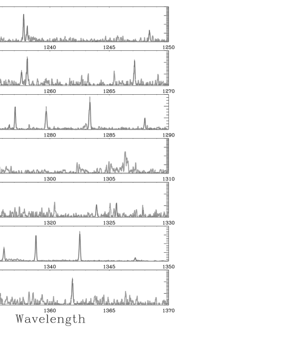
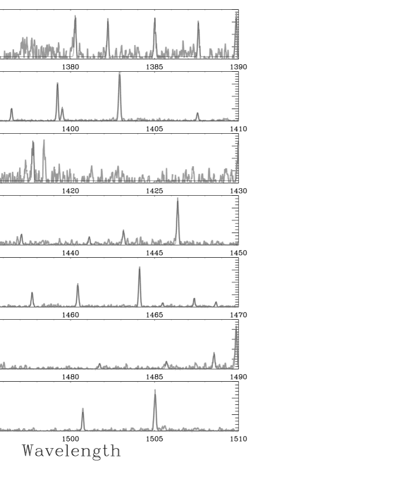
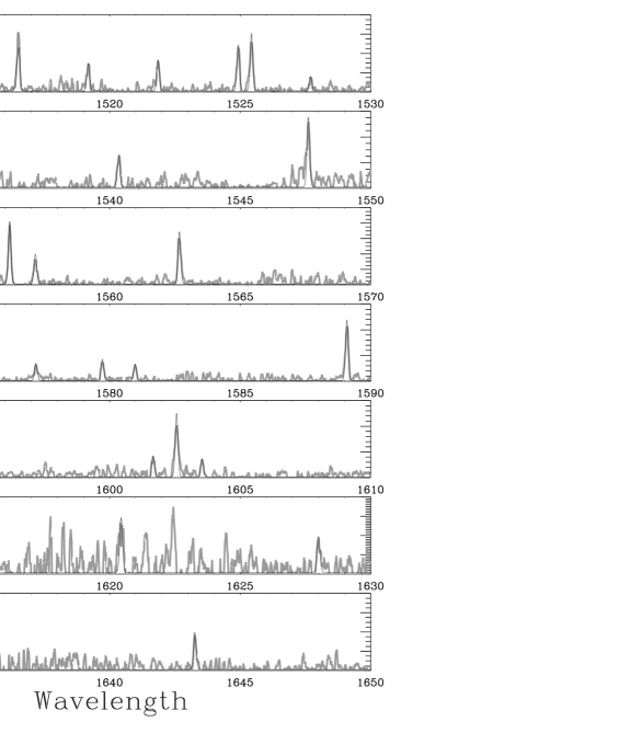
Figure 1 shows the spectral region between 1230 Å and 1650 Å containing all of the H2 lines detected in the STIS E140M spectrum, which in the figure are fitted with Gaussians. All of the lines can be identified as members of various Lyman band sequences fluoresced by the H I Ly line. The Ly emission from Mira B excites H2 from various rovibrational states in the ground electronic state () to the excited Lyman band electronic state (). From there the H2 molecules radiatively deexcite back to the ground electronic state, resulting in the rich H2 line spectrum observed by HST. We use the Abgrall et al. (1993) listing of Lyman band H2 rest wavelengths and transition probabilities to identify the lines. To conclusively identify a fluorescence sequence, we require that at least two lines of the sequence be detected with relative strengths roughly consistent with the transition probabilities. In this manner, we identify 13 fluorescence sequences with 13 different H2 transitions within the H I Ly line. These sequences successfully account for all of the clearly detected narrow lines in the Mira B E140M spectrum.
In Table 1, we provide a complete listing of all 103 positively detected H2 lines, which are grouped into fluorescence sequences. For H2 Lyman band transitions, the dipole selection rules require , where and are the upper and lower rotational quantum numbers, respectively. The line ID’s in Table 1 use the standard notation, where and are the upper and lower vibrational quantum numbers, respectively, and for or for .
Table 2 lists information on the fluorescing transitions within the Ly lines, including rest wavelengths (), absorption strengths (f), and the energies () and statistical weights () of the lower levels of the transitions. Also listed is the total flux fluoresced within each sequence (), in units of ergs cm-2 s-1 (see §2.2). The dissociation fraction per excitation (from Abgrall, Roueff, & Drira, 2000) is listed for each sequence (), as is a total dissociation fraction based on our best model of the H2 line ratios (; see §2.2).
We measure fluxes for all the lines using Gaussian fits to the lines, as shown in Figure 1. When we fit the lines simultaneously, forcing all lines to have the same centroid velocity and line width, we find an average centroid of km s-1, consistent with the central velocity measured for Mira’s circumstellar shell of about 56 km s-1 (Bowers & Knapp, 1988; Planesas et al., 1990; Josselin et al., 2000). The measured line fluxes listed in Table 1 are from a fit in which the centroids were allowed to vary but the line widths are still forced to be the same. The H2 line width measured in this fit is km s-1, after correction for the E140M line spread function from Sahu et al. (1999).
We then tried a different fit to the data to see if the line ratios within the 13 fluorescence sequences are consistent with the transition branching ratios from Abgrall et al. (1993). We simultaneously fitted all of the lines, forcing all to have the same centroid velocity and line width, but we also forced the line flux ratios to be consistent with the transition probabilities. What this means is that besides the average line centroid and line width, the only other free parameters of the fit are 13 flux normalization factors for the 13 sequences of lines. The result is shown in Figure 2, where a smoothed representation of the entire E140M spectrum is compared with the best fit. The fit is very poor, with the discrepancy between the observation and model clearly being wavelength-dependent. In particular, the shorter wavelength lines are observed to have lower fluxes relative to the longer wavelength lines than the transition probabilities suggest.
We believe that this is due to an opacity effect. We will show in §2.3 and §2.4 that there are actually visible H2 absorption features within the Ly line where some of the H2 sequences are being pumped. This means that the H2 lines being fluoresced have significant opacity. Lower wavelength lines are transitions to lower vibrational levels than the higher wavelength lines. The lower vibrational levels will have higher populations if the levels are thermally populated, so the lower wavelength lines should have higher opacities, thereby explaining why they have systematically lower fluxes than the transition probabilities predict.
2.2 Radiative Transfer Simulations
In order to determine whether opacity effects can in fact explain why the observed H2 line ratios are different from the transition branching ratios, we perform Monte Carlo radiative transfer simulations, which we now describe in detail. The fact that we see the H2 in absorption within Ly (see §2.3 and §2.4) suggests that we see the Ly emission through an H2 layer. Thus, in our model we construct a plane-parallel slab of H2 with an assumed H2 column density, , and temperature, T. We assume Ly emission is normally incident on one side of the slab, with our observations being made from the other side of the slab.
The wavelength dependent opacity of the slab to a given H2 transition from a lower level with column density, , is (in cgs units)
| (1) |
where is the oscillator absorption strength of the transition and is a Voigt line profile function with a width appropriate for the assumed temperature. We compute the f-values from the transition probabilities of Abgrall et al. (1993), using the relation between the two from Abgrall & Roueff (1989). Assuming the H2 levels are thermally populated, the column density of H2 at a given level, , depends on both and T, and can be computed from the following equation:
| (2) |
where is the energy of the lower level of the H2 transition (in cm-1) and is the statistical weight of this level. The H2 energy levels that we assume are from Dabrowski (1984). The statistical weights are computed from the equation
| (3) |
where I is the nuclear spin, which is 0 for even and 1 for odd (Morton & Dinerstein, 1976). Note that Table 2 lists , , and values for the fluorescing transitions within Ly.
We model the line ratios of each fluorescence sequence separately. For the sequence fluoresced by the R(6) transition (see Table 1), for example, we numerically send Ly photons across the absorption line profile () of the R(6) line. In the Monte Carlo routine, the number of optical depths a photon travels before scattering is the negative natural logarithm of a random number generated between 0 and 1. When this number is less than the H2 optical depth of the slab seen by the Ly photon, the photon is absorbed by the H2. The excited H2 molecule then either deexcites or is dissociated. We use the dissociation probabilities of Abgrall et al. (2000) to indicate the fraction of excitations to the Lyman band that result in dissociation (), which are listed in Table 2 for each sequence.
If the molecule radiatively deexcites, the result is an H2 emission photon. We use the transition probabilities of Abgrall et al. (1993) to indicate how the photons are to be distributed among the various lines in the sequence (i.e., the R(6) and P(8) sequences for the example sequence mentioned above). We randomly determine a new location for the photon within the line profile () assuming complete frequency redistribution to establish the probability distribution. We also randomly determine a new direction for the photon assuming complete angular redistribution.
We compute the H2 opacity for the new photon to escape the slab based on where it is in the slab, what particular line it is in, where it is in the line profile, and what direction it is traveling, and then we repeat the process of determining whether the photon escapes the slab or is absorbed by an H2 molecule again. Photons that ultimately scatter back towards the Ly source are discarded. Photons that scatter out the other end of the slab towards the observer are counted. By numerically sending enough photons through the slab for each of the 13 fluorescence sequences, we can determine what the line ratios will be for each sequence, for comparison with the observed line fluxes. We use a separate fitting routine to determine the best 13 normalization factors to convert the model photon counts to the observed line fluxes of the 13 fluorescence sequences. We perform this whole simulation for a range of assumed T and values.
Figure 3 displays contours showing the quality of the fit to the data as a function of T and . The best fit is for K and and has . The temperature and column density are highly dependent on each other, however, and Figure 3 shows that there is a long trough in the contours, implying that uncertainties in and could be large. Because systematic uncertainties surely dominate this type of analysis, we do not attempt to quote error bars based on the values. However, in the following sections we will present two other arguments for these measurements being reasonable and consistent with the data. In any case, 3600 K is a plausible temperature for the H2 in the sense that the temperature is not so high that the H2 should be collisionally dissociated.
Figure 4 shows the model spectrum for the best fit from our simulations, compared with the observed spectrum. Comparing Figure 4 with Figure 2 reveals that taking into account opacity effects can indeed remove the large wavelength dependent discrepancy noted above. However, there are still some discrepancies between the model and the data that are more easily seen in Figure 5, which compares the fluxes of this best model with the observed fluxes. There are many data points that lie farther from the data-model agreement line than the 1 measurement uncertainties indicated in the figure. The model line fluxes are also listed in Table 1 in order to indicate explicitly which lines fit well and which do not.
In Figure 6, we plot the flux discrepancies between the best model and the data (in standard deviation units) as a function of wavelength. Lines in fluorescence sequences that are excited from low energy levels ( cm-1) are shown as open boxes and lines of fluorescence sequences excited from high energy levels ( cm-1) are shown as filled boxes. (The values for all the sequences are listed in Table 2.) It is apparent that the low energy lines are systematically more discrepant than the high energy lines. It is tempting to claim that this might be evidence of multiple H2 temperature components, since in principle the low energy lines could be excited at lower temperatures than the high energy lines. However, there is no obvious wavelength dependence in the flux discrepancies that would suggest that the estimated value is inaccurate for the low energy lines, and when we perform the analysis described above considering only the low energy lines we do not obtain significantly different results — the large discrepancies for the low energy lines remain. Therefore, it is uncertain what is indeed responsible for this behavior, but perhaps the lower energy levels of H2 are not solely populated by thermal collisions.
Our best fit to the data, which is shown in Figure 4, provides us with measurements of the total flux fluoresced by each of the 13 fluorescence transitions within Ly, , which are listed in Table 2. These total fluoresced fluxes include the fluxes of lines within each sequence that are undetected either because they are too weak or because they lie outside the observed spectral range. We can include these unobserved fluxes because our fit makes predictions for what the fluxes of these lines should be. Our fit also tells us the fraction of fluorescences that lead ultimately to dissociation of an H2 molecule rather than the emergence of an H2 emission photon. This is recorded in the dissociation fraction, , in Table 2. The fraction is naturally larger than the dissociation fraction per excitation, , because the H2 opacity sometimes results in multiple excitations before an H2 photon either escapes or dissociates an H2 molecule.
2.3 Deriving the Ly Profile Seen by the Fluoresced H2
The amount of Ly flux absorbed by a given H2 transition depends in part on the amount of H I Ly flux overlying the transition (). An absorption line profile, , can be expressed as
| (4) |
where the opacity profile, , is given by equation (1). After accounting for the fraction of H2 fluorescences that lead to dissociation rather than an H2 photon, the total emission observed from a fluorescence sequence () will be equal to the absorbed flux along a line of sight if the H2 that is being fluoresced completely surrounds the star and the H2 emission emerges isotropically. The emission will be less than this if the H2 only partially surrounds the star, or if the H2 emission is preferentially scattered away from our line of sight toward Mira B. The emission could be greater if the emission is preferentially scattered toward our line of sight. Thus,
| (5) |
where is a correction factor meant to account for inaccuracies in the assumptions of uniform H2 coverage and isotropic emission. If the emission is assumed isotropic, is then simply a number between 0 and 1 representing the H2 coverage fraction. The factor corrects for dissociations, and the values can be found in Table 2. Combining equations (4) and (5),
| (6) |
Table 2 lists values for our 13 fluorescence sequences. The opacity profile of the line being fluoresced, , can be computed from equations (1)–(3), where Table 2 lists the , , and values for the fluorescing transitions. Assuming the K and values derived in the previous section, we can then compute values from equation (6) for each of our fluorescence sequences.
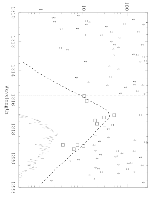
These quantities should map out the Ly profile that is seen by the H2, when plotted as a function of the wavelength of the fluorescing transition. This is what the boxes indicate in Figure 7, which demonstrates that the values do indeed map out a reasonably self-consistent line profile, although there is still some scatter. We interpolate between the boxes (and extrapolate beyond them) to obtain the dashed line in figure. The H2 flux fluoresced by the 0-2 R(2) line at 1219.09 Å is low based on Figure 7. This is likely caused by the blending of this line with the 2-2 R(9) line at 1219.10 Å, which results in the 2-2 R(9) line shielding the 0-2 R(2) line from the full Ly flux at that wavelength.
Figure 7 compares the H I Ly profile seen by the H2 (dashed line) with the Ly profile that we actually observe in our STIS data (dotted line). There appear to be absorption features within this profile, some of which line up with the H2 lines. We will return to this issue in the next subsection. Both the observed and derived Ly profiles in Figure 7 are almost entirely redward of the rest frame of the star, which is the vertical dot-dashed line in the figure. As discussed in Paper 1, the Mg II h & k lines of Mira B show a similar behavior, and the cause is presumably a fast wind from Mira B that absorbs the blue side of the line. The fact that the profile seen by the H2 also has no emission on the blue side means that the wind absorption happens before the Ly emission encounters the H2, which is an important clue to the location of the H2 being fluoresced.
There are many other H2 transitions between 1210 Å and 1222 Å that could potentially have been fluoresced, if the lower levels had been populated and if there was sufficient background flux at the appropriate wavelength. Thus, we estimated upper limits for the fluoresced flux from these transitions and these upper limits are used to compute the upper limits to shown in Figure 7. To be more precise, for each undetected fluorescence sequence we identify the easiest to detect line within the sequence by dividing the transition probability of each line by the flux error of our observed spectrum at the wavelength of that line — the line with the largest value is assumed to be the easiest to detect. We estimate a conservative upper limit for the flux of this line and then extrapolate that flux to a total fluoresced flux () assuming the line ratios within the sequence are those suggested by the transition probabilities. This does not take into account the opacity effects that we see in the detected sequences, but as long as we are conservative in our initial flux upper limit the final total flux upper limit should be acceptable. Using this upper limit for , we can then compute an upper limit for from equation (6). We correct for dissociation assuming , which is roughly what we see for our detected sequences in Table 2. In this way, we compute all the upper limits shown in Figure 7.
There are two important results from the upper limit calculations. The first is that there are no upper limits beneath the boxes that would suggest nonthermal populations (i.e., there are no levels that should have been thermally populated at K but are not). The second is that there clearly are transitions that would have been fluoresced by the blue side of the Ly line if the flux on that side of the line was comparable to that on the red side. This confirms the conclusion stated above that the blue side of the Ly line must be absorbed before the Ly emission encounters the H2.
The relatively self-consistent, smooth Ly profile suggested by the boxes in Figure 7 implies that the K and values derived in the previous section and assumed in the derivation of the Ly profile are reasonably accurate measurements. If these values were wildly inaccurate or if the H2 energy levels were not thermally populated at all, then the boxes would not line up like they do in Figure 7. Figure 8 shows what happens if we arbitrarily assume temperatures of 2600 K and 4600 K in this analysis instead of 3600 K. For the low temperature case (Fig. 8a), the scatter in the data points clearly increases compared to Figure 7. For the high temperature case (Fig. 8b), some of the upper limits fall too low.
We do not expect our derived Ly profile in Figure 7 (dashed line) to precisely reproduce the observed profile (dotted line) for two primary reasons: 1. The Ly profile could suffer from additional circumstellar and/or interstellar H I absorption after it encounters the H2 region that is fluoresced, making the observed profile lower than the derived profile. 2. The geometrical correction factor could be different from one. Since the observed profile is lower than the derived profile, additional absorption of Ly (case #1) is a distinct possibility. Conclusive evidence of additional absorption beyond the H2 region is provided by the simple fact that there are two fluoresced transitions near 1216 Å where there is no observed Ly flux whatsoever.
We now try to determine if interstellar or circumstellar absorption alone can account for the difference between the observed and derived Ly profiles in Figure 7. In order to do this, we first have to estimate the centroid and temperature of the absorbing material for both the ISM and circumstellar absorption cases. The local cloud flow vector of Lallement et al. (1995) predicts a heliocentric velocity for the ISM absorption of 18.6 km s-1. For a line of sight as long as that towards Mira there will undoubtedly be many ISM absorption components that will cause the actual centroid of the ISM absorption to differ significantly from this value, but the value should nevertheless be accurate enough for our purposes. For the ISM temperature, we assume a typical temperature for warm ISM material of 8000 K (e.g., Wood & Linsky, 1998). For circumstellar material, which should be expanding only very slowly, we assume a heliocentric velocity equal to Mira’s estimated radial velocity of 56 km s-1, and we assume a cold temperature of 500 K.
Based on these assumptions, in Figure 9a we show the ISM and circumstellar absorption that results from column densities of , 20.5, and 20.7. The ISM and circumstellar absorption profiles are very similar, emphasizing the fact that at column densities this high the absorption profiles are not very dependent on either the temperature or centroid velocity. However, none of the column densities results in an acceptable fit to the data. There is simply too much absorption in the far red wing. When column densities are raised high enough to account for it, there is then way too much absorption between 1217 and 1219 Å. The only way we can think of rectifying this situation is to assume that our correction factor, , is greater than one. This could mean that the H2 emission is for some reason preferentially scattered into our line of sight to Mira B, meaning we should scale the model Ly profile downwards. It could also mean that the Ly flux is preferentially scattered out of our line of sight, which would mean we should scale our observed Ly profile upwards. We will discuss these two possibilities in more detail below (see §2.5). For now, we assume the latter possibility is the case and by trial and error we find that we can best fit the data when we scale the observed Ly profile upwards by a factor of 2.5 (i.e., ), in which case a column density of yields a reasonable fit to the data, as shown in Figure 9b.
In the figure, the ISM absorption fits a little better than the circumstellar absorption. We attach no importance to this, however, since the fit to the circumstellar absorption can be improved by slight adjustments to the flux scaling factor or value. An estimate of the mass of Mira’s circumstellar envelope presented by Bowers & Knapp (1988) from observations of the H I 21 cm line suggests a circumstellar column density of only , which is much too low to account for the observed H I absorption. We have some concerns that trying to estimate the amount of circumstellar H I from the 21 cm emission could result in an H I mass that is much too low, since the lifetime of the 21 cm transition ( yrs) is so much greater than the crossing time across the circumstellar envelope ( yrs for a typical expansion velocity of 5 km s-1), meaning that much of the H I that is collisionally excited will actually leave the envelope before emitting a 21 cm photon. Thus, we do not completely rule out the possibility that the H I absorption is circumstellar.
As for the possibility that the H I absorption is interstellar, the column density of is not impossibly high for Mira’s distance of 128 pc. Mira is likely to be outside the Local Bubble (where ISM column densities are quite low) based on the Local Bubble maps estimated by Sfeir et al. (1999) from Na I column density measurements. One of the stars in their list that is near Mira’s location (, , d=128 pc) is HD 14613 (, , d=121 pc), which shows a high Na I column of , probably corresponding to an H I column well above cm-2 (Sfeir et al., 1999).
2.4 The Evolution of the Ly Profile During its Journey Towards Earth
In Figure 10, we present a model of how the Ly profile evolves along the line of sight from Mira B to HST based on the results of the previous subsection. The starting point of the model is the solid line in Figure 10a, which is simply the dashed line from Figure 7. As described above, this is the profile seen by H2 after Mira B wind absorption has already absorbed the blue half of the profile. The H I Ly opacity in the wind figures to be so high that scattering will erase all memory of the original Ly profile, but we can at least obtain a schematic representation for the original profile by reflecting our derived profile from Figure 7 onto the blue side and then extrapolating between the peaks. The result is the dotted line in Figure 10a.
Thus, the accretion disk around Mira B produces a Ly profile that looks schematically like the dotted line in Figure 10a. Mira B’s wind erases the blue side of the profile, resulting in the solid line profile in Figure 10a. The Ly emission then encounters the K, H2, resulting in narrow H2 absorption features within the Ly profile, as shown in Figure 10b. The Ly emission then makes the long journey through both Mira’s large circumstellar envelope and the ISM. This results in worth of Ly absorption, the effects of which are illustrated in Figure 10c. The resulting profile is smoothed with the instrumental profile appropriate for our STIS E140M observation, and in Figure 10d that profile is compared with the observed Ly profile multiplied by a factor of 2.5 (see §2.3). Our best model of the H2 line ratios predicts that some of the Ly flux that is absorbed by the H2 will naturally be reemitted in the H2 lines within Ly that are being fluoresced (see, e.g., Fig. 4). Thus, when comparing the observed Ly profile with the model, we first remove the H2 emission component from the Ly profile by subtracting the H2 emission line fluxes predicted by our model from the observed profile. This is only a minor correction, but it does slightly deepen the apparent H2 absorption features within the observed Ly profile that were noted above. Finally, as noted above the observed profile is multiplied by a factor of 2.5 to match the fluxes of the model profile in Figure 10d. Both profiles in Figure 10d were smoothed additionally by a 5-bin boxcar in order to reduce noise in the observed Ly line.
The observed Ly profile does suggest the presence of absorption features where the model suggests there should be H2 absorption (see Fig. 10d), validating our initial assumption that the fluoresced H2 does indeed lie at least in part between us and Mira B. The K and measurements based on the result from Figure 3 slightly overpredict the amount of observed absorption for most lines. Based on the H2 absorption alone, we would estimate an H2 column density along the observed line of sight to be more like (assuming K naturally). There could in principle be a difference between the amount of H2 along the line of sight we are observing and the average line of sight from Mira B. However, the observed amount of absorption is consistent enough with that predicted by the model to provide further support for the K and measurements from the line ratio analysis.
2.5 The Discrepancy Between the Observed Ly and H2 Fluxes
One aspect of our analysis of the H2 lines that has yet to be explained is this factor of 2.5 that we must multiply the observed Ly profile by in order to be able to account for the amount of H2 emission produced by Ly fluorescence (see Fig. 9). Why do we observe weaker Ly fluxes than the H2 must see? There were 2 basic possibilities suggested above in §2.3. One is that the H2 emission is preferentially scattered into our line of sight, and the other is that the Ly emission is preferentially scattered out of our line of sight.
One way the first possibility might occur is if there is an optically thick H2 layer of some sort behind both the Ly source and the H2 layer seen in absorption within Ly. Such a background layer could act to scatter all the H2 emission back in our direction. This would mean that if Mira B were observed from the opposite direction, from the actual line of sight, little if any H2 emission would be observed, whereas in our line of sight we would see about twice as much H2 emission as would be observed if the emission was isotropic. The problem with this scenario is that the backscattering H2 layer would have to have a high enough column density that it should produce more H2 flourescence sequences than we actually observe. In essence, one would have a situation analogous to Figure 8b, where the upper limits are becoming inconsistent with the detections. There does not seem to be an easy way to preferentially scatter H2 into our line of sight without introducing this problem.
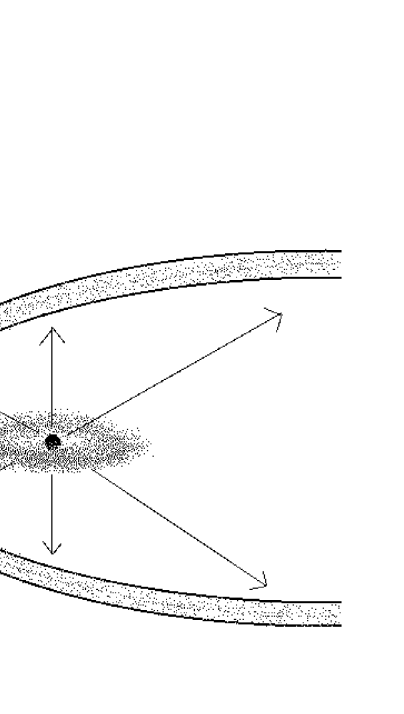
This is why we prefer the second possibility mentioned above, that the Ly emission is preferentially scattered out of our line of sight. The most likely scenario for how this could happen has to do with the possibility that we are observing Mira B’s accretion disk close to edge-on, much as it is depicted in Figure 11. The orbit of Mira B around Mira A is poorly known. Prieur et al. (2002) have derived a new orbit that is more consistent with recent observations (Karovska et al., 1993) than an older estimate from Baize (1980). The Prieur et al. (2002) orbit suggests an orbital period of 498 days and an inclination angle of . Assuming that the accretion disk lies in the same plane as Mira B’s orbit, the disk is then observed only from edge-on. However, since observations currently cover only about 15% of the orbit, the Prieur et al. (2002) orbit must still be considered very uncertain at this point.
Nevertheless, if the accretion disk is close to edge-on there are two ways that the Ly emission could be suppressed along our line of sight. One is that dust in the disk extends high enough above the plane of the disk to extinct the observed Ly emission by a factor of 2. In this scenario, most of the H2 being fluoresced will be above the polar regions of the disk and will see the Ly emission without any extinction, thereby explaining why the H2 emission fluxes seem higher than the observed Ly fluxes would predict. A second possibility relies on the fact that Mira B’s Ly emission has to pass through a wind that is extremely opaque, which accounts for the highly redshifted nature of the emission that ultimately emerges (see Fig. 7). If H I densities in Mira B’s wind are significantly higher closer to the plane of the disk, this could mean that the Ly emission preferentially escapes in less opaque polar directions, explaining why we see less flux in our supposed edge-on line of sight. Ardila et al. (2002b) present evidence that T Tauri star winds are in fact denser near the accretion disks.
2.6 The Location of the Fluoresced H2: The Wind Interaction Region?
There are basically two possible locations for the observed H2 that we consider. One is that the H2 is in the outer regions of the accretion disk, and the other is that the H2 is within the wind of Mira A. Fluoresced H2 emission observed from T Tauri stars can apparently be either unresolved emission from the accretion disk, or emission from an outflow, in which the H2 may be circumstellar material entrained in the wind (Ardila et al., 2002a; Herczeg et al., 2002). For T Tauri itself, the H2 emission is clearly extended and is therefore probably circumstellar (Brown et al., 1981; Herbst, Robberto, & Beckwith, 1997).
For Mira B, there are several factors that make the accretion disk interpretation less attractive. One is the presence of H2 absorption within the Ly line, meaning the disk H2 would have to exist above the disk far enough to extend into our line of sight. Furthermore, in such a situation one would expect since the disk H2 would only intercept a small fraction of the total Ly emission. The actual value of ( from §2.3) is more consistent with the H2 completely surrounding the star, which is difficult to reconcile with a disk interpretation. The narrow widths of the H2 lines may also be a problem. As discussed in §2.5, the disk is observed only from edge-on based on the Prieur et al. (2002) orbit, so if the H2 lines were in the disk their widths should be at least as broad as the rotational broadening provided by disk rotation. If the mass of Mira B is M⊙, the observed width of the H2 lines ( km s-1) would suggest a distance from the star of at least 1.1 AU, assuming Keplerian rotation. The disk would have to be flared significantly to expose parts of the disk this far out to the Ly emission. One might also expect rotationally broadened line profiles to be non-Gaussian, but they are in fact Gaussian in shape.
Thus, we believe that the H2 is more likely to be within Mira A’s wind, which will surround the star (consistent with ) and will be beyond the Mira B wind absorption region, consistent with our finding from Figure 7 that the H2 fluorescence must come after Mira B’s wind absorbs the blue half of the Ly line. Hydrogen in Mira A’s massive wind should be largely molecular (Bowers & Knapp, 1988), but it should be significantly colder than the H2 temperature of K that we derive. Thus, the H2 in Mira A’s wind must be heated somehow as it approaches Mira B. One possibility is that the H2 is heated by its interaction with the hotter and faster, but less massive wind of Mira B, placing the fluoresced H2 in the interaction region between the two winds, as shown schematically in Figure 11.
In order to ascertain what the wind interaction region of the Mira binary system might be like, it is necessary to review what is known about the winds of the 2 stars. There have been many estimates for Mira A’s mass loss rate and wind velocity from observations of CO, H I, and Ca II in Mira’s circumstellar environment. The mass loss estimates have generally fallen in the range — M⊙ yr-1, and wind velocities have generally been quoted as km s-1 (Yamashita & Maehara, 1978; Knapp, 1985; Bowers & Knapp, 1988; Planesas et al., 1990; Knapp et al., 1998; Ryde & Schöier, 2001).
The accretion rate onto Mira B that results from Mira A’s wind has been estimated to be about — M⊙ yr-1, which can account for Mira B’s total luminosity of about 0.2 L⊙ (Warner, 1972; Jura & Helfand, 1984; Reimers & Cassatella, 1985). The accretion rate provides an upper limit for Mira B’s mass loss rate. However, although the existence of Mira B’s wind has been noted before on the basis of absorption within the H I Balmer lines (Yamashita & Maehara, 1977), there has been no estimate made for the mass loss rate. Thus, we now derive our own estimate.
Probably the best diagnostics for Mira B’s wind are the Mg II h & k lines at 2800 Å. Our 1999 STIS observations include an observation with the moderate resolution E230M grating of the 2303–3111 Å region containing Mg II, and IUE observed the Mg II lines many times with its high resolution grating. In Figure 12, we show the Mg II k line profile observed by STIS, and a typical Mg II k line profile observed by IUE (LWP 29795 from 1994 December 30), both plotted on a velocity scale centered in the stellar rest frame. These spectra were also presented in Paper 1. Both Mira A and Mira B are in the aperture for the IUE observations and emission from Mira A is occasionally seen by IUE at certain pulsation phases (see, e.g., Wood & Karovska, 2000), but for the spectrum in Figure 12b all the emission is from Mira B.
The IUE spectrum shows saturated wind absorption between 0 and km s-1. The IUE data set of 28 high resolution spectra containing Mg II shows that the Mg II emission and the wind absorption are clearly variable, with the extent of the absorption varying between and km s-1. However, the absorption is always very opaque, in contrast to the STIS Mg II line, which only shows opaque absorption up to km s-1 and less opaque absorption beyond that to km s-1. This difference suggests a significantly lower mass loss rate at the time of the STIS observations. This is consistent with the dramatically lower UV line and continuum fluxes observed by STIS (see Fig. 12), which suggest a lower accretion rate that would naturally be expected to result in a lower mass loss rate (see Paper 1).
The wind “absorption” features are actually a result of scattering within the line profile. Nevertheless, to simplify the analysis we treat the wind features as pure absorption features. We first approximate the line profile above the absorption features as shown in Figure 12 for both the STIS and IUE spectra. The amount of flux removed by the wind beneath these estimated background profiles is then indicative of the amount of mass in the wind.
We assume a radial wind with a density profile given by
| (7) |
where is the assumed mass loss rate and is the wind velocity. Following previous analyses of wind absorption (e.g., Harper et al., 1995), we assume is a power law of the form
| (8) |
where is the terminal velocity and is the radial distance where the wind acceleration is initiated. In stellar wind calculations one would normally assume that the wind is accelerated near the surface of the star and that should therefore be the radius of the star. However, it is not known for sure if Mira B is a white dwarf or a red dwarf (see §1), so its radius is very uncertain, but even if Mira B’s identity was clearly known it is not certain that an accretion induced wind would originate from close to the star.
Our mass loss rate estimates will be proportional to the assumed value, so the issue is not purely academic. We will assume R⊙, which seems to yield reasonable density profiles and mass loss rates. It seems natural to assume that the wind is likely to originate in hot, rapidly rotating, interior regions of the accretion disk, and we note that R⊙ roughly corresponds to the radius where Reimers & Cassatella (1985) place the origin of the Si III] 1892 and C III] 1908 lines, assuming the widths of these lines are determined by Keplerian rotation around a 0.6 M⊙ accretor.
We vary the , , and parameters to see which yield the best fits to both the STIS and IUE lines in Figure 12. In order to derive a Mg II density profile from the total density profile, , we assume a solar abundance for Mg (Anders & Grevesse, 1989), and we also assume that Mg II is the dominant ionization state of Mg in the wind. Since Mira is an evolved star system, it is possible that Mg abundances are higher than solar, in which case our mass loss rates will be too high. However, it is possible that a significant fraction of the Mg could be in an ionization state other than Mg II, in which case our mass loss rates could also be too low. The Mg II flow velocity along the line of sight is naturally provided by equation (8). The last thing we have to assume to compute Mg II absorption along the line of sight is a Doppler broadening parameter, , for the absorption, which will be characteristic of the thermal and turbulent motions of the Mg II atoms. We would expect thermal broadening appropriate for the temperature of formation of Mg II to limit to be greater than 2 km s-1. When we assume km s-1, the wind absorption broadens to velocities greater than 0 km s-1, inconsistent with the absorption features seen in Figure 12. Thus, we believe km s-1, and our results are not terribly sensitive to the assumed within this range. Our best fits in Figure 12 assume km s-1.
The STIS data yield a much more precise mass loss measurement than the IUE data, because the wind absorption is not saturated. Thus, we focused most of our initial efforts in fitting the STIS data. Figure 12a shows our best fit to the STIS Mg II profile, which assumes M⊙ yr-1, km s-1, and . Continuum fluxes and Mg II fluxes are about a factor of 20 higher in the IUE spectrum in Figure 12b. Thus, we assume is a factor of 20 higher as well ( M⊙ yr-1), and Figure 12b shows that we can fit the IUE data nicely with this value if we assume km s-1, with the parameter remaining at .
Our mass loss estimates demonstrate that the wind absorption features are entirely consistent with Mira B’s mass loss being lower by about a factor of 20 at the time of the STIS observations relative to the IUE era, consistent with the decrease in accretion rate suggested by the factor of decrease in UV line and continuum flux. Based on the data currently available, the Mg II profile in Figure 12b appears to be more typical for Mira B both in terms of its flux and its wind absorption, so the M⊙ yr-1 value estimated from this profile is probably a more typical value for Mira B than the lower value measured from the STIS data. This value and the previous estimates for Mira B accretion rates mentioned above ( M⊙ yr-1) suggest that about 1% of the mass accreting onto Mira B is ejected into the wind.
Now that we have mass loss and wind velocity estimates for Mira B, we can estimate a location for the wind interaction region for the Mira binary system, which will be roughly where the wind ram pressures (i.e., ) are equivalent. The ratio of wind ram pressures at a point equidistant from the two stars can be expressed as
| (9) |
where and are the mass loss rate and terminal velocity for Mira A’s wind, and and are the mass loss rate and terminal velocity for Mira B’s wind. Equation (7) indicates how the wind density will fall off with distance from the star, if the wind velocities are set equal to the terminal velocities. For , the distance from Mira B toward Mira A at which the wind ram pressures will balance is
| (10) |
where is the distance between the two stars. With a separation of and a distance from Earth of 128 pc (Karovska et al., 1997; Perryman et al., 1997), the projected distance between Mira A and B is 70 AU. The orbit of Prieur et al. (2002) mentioned in §2.5 suggests that the projected distance should be close to the actual distance, so we will assume AU, although we note once again that the Prieur et al. (2002) orbit is uncertain and anything derived from it is therefore somewhat suspect.
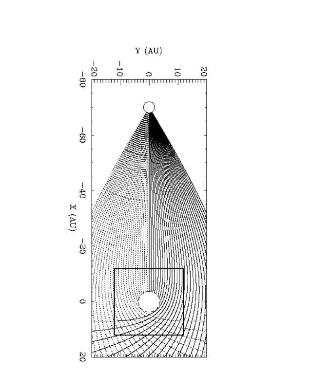
The terminal wind speed for Mira A is roughly km s-1, but its actual speed at the wind interaction region will be somewhat higher, because the wind will accelerate as it falls into Mira B’s gravitational well. In Figure 13, we show particle trajectories for Mira A’s wind, assuming it flows from Mira A at a speed of km s-1 and then is influenced only by the gravitational field of Mira B, assuming a Mira B mass of 0.6 M⊙. The trajectories are truncated at a distance of 3.7 AU from Mira B, because by trial and error we determine that this is roughly the location of the wind interaction region based on the following line of reasoning. At this distance from Mira B along the line toward Mira A, the Mira A wind speed has increased to 13 km s-1. If we therefore assume km s-1 and M⊙ yr-1, and we assume M⊙ yr-1 and km s-1 from our IUE measurements (see Fig. 12b), from equations (9) and (10) we then compute AU, demonstrating self-consistency with the location where we estimated .
Figure 13 indicates that all Mira A wind material ejected within of the direction of Mira B ends up within 3.7 AU of Mira B, corresponding to about 0.5% of Mira A’s total wind mass. If this material is accreted onto the star, the implied accretion rate is about M⊙ yr-1 (assuming M⊙ yr-1). This value is within a factor of 2 of the Mira B accretion rate estimated from its luminosity, providing support for AU being a reasonable size scale for the wind interaction region.
However, the accretion luminosity and Mira B mass loss rate were about a factor of 20 times lower at the time of our STIS observations. If this is due to a low density region in Mira A’s wind, then the decrease in ram pressure of Mira B’s wind presumably balances the decrease in Mira A’s wind, and our estimate of above does not change. If, however, we assume that the decrease in accretion luminosity is due to a temporary instability rather than a change in Mira A’s wind properties, and if we also assume that the wind interaction region has had time to respond to the lower Mira B mass loss rate, then our estimate of decreases to AU. More precisely, at 0.4 AU the Mira A wind speed should have increased to 38 km s-1, so if we assume km s-1 and M⊙ yr-1, and we assume M⊙ yr-1 and km s-1 from our STIS measurements (see Fig. 12a), from equations (9) and (10) we then compute AU.
Thus, for the wind interaction interpretation of the H2 emission, we estimate that the H2 is at a distance of roughly AU from Mira B, depending on what role variations in Mira A’s wind have played in Mira B’s dramatic decrease in luminosity, and on whether the wind interaction region has had time to react to the decrease in Mira B’s mass loss rate. However, the closer the H2 is to Mira B, the faster it is expected to be moving, and therefore the closer the vector from Mira A to Mira B has to be to the plane of the sky in order to explain why the H2 lines are not shifted significantly from the Mira rest frame (see §2.1). Mostly for this reason, we suspect AU is more likely than AU. In any case, the size scale of the wind interaction region is small enough that it should not be resolvable with STIS. The STIS aperture used for our observations has a projected size of AU at Mira’s distance, and is shown schematically in Figure 13.
In Figure 14, we show the spatial profile of the geocoronal H I Ly emission (solid line), which fills the aperture and therefore has a broad, square-topped appearance. (The geocoronal Ly line was mentioned in Paper 1, but is removed before displaying the Ly spectrum in Figs. 7–10.) The geocoronal profile is compared with the spatial profile of the stellar Ly emission (dotted line) and the spatial profiles of two of the strongest H2 features: the 0-4 P(3) line and the blend of the 0-5 R(0) and 0-5 R(1) lines at 1394 Å (dashed and dot-dashed lines, respectively). There is no significant difference between the stellar Ly and H2 profiles in Figure 14 that would indicate that the H2 emission is spatially resolved, and all three profiles are significantly narrower than the geocoronal profile. We estimate that the radius of the H2 emission region can be no larger than about 6 AU to be consistent with its unresolved nature. Our estimates above for the wind interaction region distance are safely below this number.
For a Mira A mass loss rate of M⊙ yr-1 and a wind flow pattern like that in Figure 13, the Mira A wind density at the wind interaction region 3.7 AU from Mira B should be about gm cm-3, taking into account the increase in wind speed and the focusing effect of Mira B’s gravitational field. If we assume that all of this is H2, then the implied H2 number density is cm-3. Our analysis in §2.2 suggests a column density of for the fluoresced H2. The observed H2 emission could therefore be explained by an interaction layer of thickness AU. This value is reasonable in that it is significantly smaller than the distance to the layer from Mira B, demonstrating that Mira A’s wind is dense enough at Mira B’s location for the “wind interaction layer” interpretation of the H2 emission to be valid.
At this point, the wind interaction interpretation for the production of the observed K H2 seems to be feasible, but problems arise when we look at the hydrodynamics of the interaction region. A shock must be present where the wind of Mira A encounters the wind of Mira B. A standard hydrodynamic shock could get to the correct temperature for a shock speed of about 1 km s-1. However, this speed is much lower than one would expect given the wind speeds involved. Furthermore, the gas cools rapidly and one expects a column density of , which is much too small. Faster shocks, in better agreement with expectations, would produce even higher temperatures and would dissociate H2 rapidly, leading to even lower H2 columns.
Hydromagnetic shocks in weakly ionized gas (i.e., C-shocks; see Draine & McKee, 1993) are observed to produce temperatures around 3000 K in Herbig-Haro objects (e.g., Gredel, 1996). It is not difficult for such a shock to provide roughly the observed T and N(H2), but a strong magnetic field and at least some ionization within Mira A’s wind are required, and it is questionable if Mira A’s cold wind can provide these initial conditions. Furthermore, the strong Ly emission from Mira B will dissociate and heat the gas beyond what is found in existing C-shock models. This leads to a somewhat different interpretation of the warm H2: a photodissociation front, in which the H2 still originates from within Mira A’s wind, but it is photodissociation that heats the H2 rather than interaction with Mira B’s wind. We now discuss this possibility in more detail.
2.7 The Location of the Fluoresced H2: A Photodissociation Front?
The importance of photodissociation of H2 by Ly is indicated by the last column of Table 2 (), which shows that for some sequences as many as 40% of fluorescence events result in dissociation rather than the escape of an H2 emission line photon. Totaling up the numbers for all sequences, one finds that 20% of all fluorescences lead to dissociation, with the 2-1 P(13) sequence accounting for 47% of these dissociations. The implied dissociation rate is cm-2 s-1, which at a distance of 128 pc corresponds to H2 atoms per second. This amounts to M⊙ yr-1, which is roughly Mira B’s total accretion rate (although once again, this accretion rate was apparently lower at the time of the STIS observations). In the previous section we envisioned the H2 being in a layer about 3.7 AU from the star. Such a layer would be completely dissociated in less than 5 days, illustrating the need for a continual source of H2. This is perhaps yet another argument in favor of Mira A’s wind being the source of the H2 rather than the accretion disk, since Mira A’s massive wind apparently does typically supply about M⊙ yr-1 to Mira B’s accretion disk.
There are two ways in which H2 fluorescence can heat the H2. For the fluorescences that lead to dissociation, the fragment H I atoms will have substantial kinetic energy that will heat the gas. Even the fluorescences that do not lead to dissociation might heat the gas since most fluorescence photons that emerge are at wavelengths redward of the Ly wavelengths where they are first fluoresced (see, e.g., Fig. 4), meaning that the fluorescence leaves the H2 in a higher net excitation state than it was in before. If this excess energy is converted to kinetic energy, the result is a net heating of the gas.
Time-dependent photodissociation in the ISM has been considered by Goldshmidt & Sternberg (1995) and Bertoldi & Draine (1996). A crucial difference is that H2 in ISM photodissociation fronts can absorb 912–1100 Å continuum photons in transitions from the lowest vibrational level, so the temperature of the gas is relatively unimportant. The H2 near Mira B, however, can only absorb Ly photons in transitions that originate in levels about 1 eV above the ground, and the populations of these levels are very sensitive to temperature. This makes the structure highly nonlinear. By analogy with photoionization fronts, a photodissociation front could produce a weak shock on its own (e.g., Shu, 1992, chapter 20).
To investigate these possibilities we have made simple numerical models of a photodissociation front surrounding Mira B. We assume constant density and speed in Mira A’s wind and simply follow the molecular fraction and temperature of the gas under the influence of the radiation field. We assume that the rovibrational levels (for and ) are in thermal equilibrium, and we compute the temperature evolution based on radiative heating of H2 and H2 radiative cooling rates from Curiel (1992). Forbidden C II and O I lines and photoelectric heating (Wolfire et al., 1995) are also included, but are not important.
For the H2 heating we use the Ly profile of Figure 10b (without the absorption features) and scale to a distance of 128 pc. For each pumping transition in Table 2, we compute the photodissociation rate using the values in Table 2 and the corresponding heating based on the fragment kinetic energies given by Abgrall et al. (2000). As mentioned above, about 80% of photoexcitations lead to an emergent fluorescent photon rather than dissociation, and whenever the fluorescent photon is longward of Ly, the H2 molecule is left in a higher state than the one which absorbed the Ly photon. Ignoring transitions to lower vibrational levels (which are likely to be immediately reabsorbed), we use the list of fluorescent transitions in Table 1 to estimate the average energy difference between the initial and final states. At low densities that increase in energy would be simply radiated away, while at high densities collisional deexcitation transfers the excitation energy back to the thermal energy of the gas. Based on the calculations of Curiel (1992) we use a rough approximation
| (11) |
where is the power deposited by photoexcitation, is the net heating of the gas, and is the H2 number density.
The strongest pumping transitions are somewhat optically thick, so we compute the optical depths assuming a 10 km s-1 line width and pure absorption. We iterate the computed temperature and optical depth structure, generally reaching convergence to a few percent in 10 or 20 iterations.
The temperature structure is highly nonlinear. Once the temperature begins to rise, the heating and dissociation rates rise rapidly until the molecules are destroyed. Sufficiently cold gas (less than about 400 K) can flow to within an AU of Mira B without significant heating or dissociation. Gas hotter than 1000 K, on the other hand, begins to experience a temperature rise and dissociation much farther out. The position of the transition depends on the balance between the flux of molecules and the flux of dissociating photons. It is easy to choose parameters that give column densities much smaller than those observed, for instance by choosing a low density or high initial temperature.
Figure 15 shows a model in which the gas is relatively cool (1000 K), so that it flows to within a few AU of Mira B before the heating becomes rapid. The left panel shows the kinetic temperature and molecular fraction of hydrogen, and the right panel shows the H2 dissociation rate and the heating rate due to fluorescence excitation and dissociation. Once the temperature begins to rise, it increases rapidly, reaching 7700 K when the gas is half dissociated. That temperature is so high that collisional dissociation, which is neglected in the model, becomes significant. This model could correspond to a flow whose temperature provides just the right heating rate to cause a transition at 3 AU (the plot shows part of a model that began at 1000 K at 3.05 AU), or it could correspond to a colder flow in which a shock or other heating mechanism suddenly raises the temperature to 1000 K at 3 AU from Mira B. The details of the initial heating are unimportant provided that the gas reaches about 1000 K. Once that happens, the excited H2 rapidly heats and dissociates. Since the photodissociation region does not have a single-valued temperature, we cannot directly compare the results of the model with our empirically estimated values of K and . Thus, in Table 3 we compare the level populations expressed as column densities predicted by the model with those suggested by K and . The overall agreement is quite good, though the highest energy levels tend to be overpopulated, suggesting that the model reaches temperatures that are too large before the molecules are destroyed. This could perhaps be due to the neglect of collisional dissociation, as mentioned above.
The model shown in Figure 15 assumes a density of cm-3 and a speed of 10 km s-1. Based on the flow pattern in Figure 13, the flow speed at the location of the photodissociation front in Figure 15 should be about 14 km s-1, roughly consistent with the assumed speed, and the assumed density corresponds to a Mira A mass loss rate of M⊙ yr-1, consistent with the range of mass loss rates quoted for Mira A in §2.6. This combination of parameters gives column densities similar to those required by the observations, so the strong lines are optically thick. The shoulders on the right sides of the photodissociation and heating rates are typical of optically thick cases. A photodissociation front naturally matches the observed column densities (optical depths of a few in the strong lines) because that condition uses all the photons available for photodissociating the gas.
Column densities significantly higher than those for our model are unlikely for any photodissociation front, because once the strong lines start to become optically thick, as they are in the model and in the observations (see, e.g., Fig. 10), essentially all available photons will be used for photodissociating and heating the gas. Higher column densities would not lead to more heating and more hot H2. Thus, the column densities listed for the model in Table 3 represent a crude upper limit for warm H2 columns that can be produced by a photodissociation front.
The fact that the observed warm H2 column density is close to this limit is a very strong point in favor of the photodissociation front interpretation of the H2. In a hydrodynamic shock situation like that discussed in §2.6, the parameters of the shock must be tuned to obtain the correct columns, whereas for a photodissociation front the observed columns are a natural product of the nature of the front. However, it is possible to choose parameters such that column densities are lower than this natural high density limit, where the photodissociation is so rapid that the lines are optically thin and many photons pass through the cool (and therefore transparent) gas outside the front without being absorbed.
Another very appealing aspect of the photodissociation front interpretation is that such a front naturally produces relative populations for the levels fluoresced by Ly with a characteristic temperature near 3500 K, because the cooler gas contributes little to the column densities of the excited rovibrational levels pumped by Ly, while the molecules have been largely destroyed in the warmer gas. Thus, the level populations of the model agree fairly well with the observed populations (see Table 3).
One possible problem with the photodissociation front interpretation is that one must propose that Mira A’s wind has a temperature of roughly 1000 K when it enters the front. This temperature is somewhat higher than the temperatures one would typically expect for Mira A’s wind. For example, Ryde & Schöier’s (2001) model of Mira’s circumstellar environment suggests a temperature of about 150 K at the distance of Mira B. Their model suggests, however, that strong infrared emission from Mira A keeps the excitation temperature of CO somewhat warmer than this, and one might expect something similar for H2. Another intriguing possibility is that the interaction between the winds of Mira A and Mira B heats the H2 enough to trigger the photodissociation front, in which case the H2 heating would be due to a combination of the wind interaction envisioned in §2.6 and the photodissociation envisioned in this section. Note that our model photodissociation front is close to the AU wind interaction distance estimated in §2.6. Another appealing feature of this scenario is that the wind interaction would decelerate Mira A’s wind. We have to assume that the Mira A wind flow toward Mira B is nearly perpendicular to our line of sight to explain why the H2 lines that we believe are formed in Mira A’s wind are not significantly shifted from Mira’s rest frame, but if Mira A’s wind is declerated by wind interaction before being fluoresced and dissociated then the constraints on the orientation of the Mira system are not as severe. In any case, the details of the initial heating of the H2 are unimportant provided that the gas reaches a temperature of about 1000 K. Once that happens, the excited H2 rapidly heats and dissociates.
The code described here is meant to demonstrate the nature or the effects of photodissociation and the associated heating. A more detailed model including a complete solution of the level populations, a more detailed treatment of radiative transfer and a hydrodynamic calculation is needed to reliably derive flow parameters. A complete model should also include collisional dissociation, as the temperatures exceed 3000 K. Nevertheless, the success of the calculations in reproducing the observed temperature and column density of the warm H2 shows that the most likely explanation for the observed fluorescence is that a cold wind from Mira A is heated within a distance of a few AU from Mira B by a photodissociation front. Any initial heating is rapidly followed by photoexcitation and photodissociation heating, so the layer of warm H2 is very thin.
As an aside, a nonlinear photodissociation front similar to those described here might operate in other situations where a strong, broad Ly emission line dominates the UV radiation field. The faint H2 infrared emission features well ahead of the main shocks in such Herbig-Haro objects as Cepheus A (Hartigan, Morse, & Bally, 2000) or HH2 (Raymond, Blair, & Long, 1997), and supernova remnants such as the Cygnus Loop (Graham et al., 1991) or RCW 103 (Oliva et al., 1999), might be signatures of the heating in a time-dependent photodissociation front. However, especially in the supernova remnant cases, photoionization may play an important role, leading to structures more closely related to those discussed by Bertoldi & Draine (1996).
2.8 Mira B’s Variability Revisited
Perhaps the biggest question about the STIS observations of Mira B concerns the fundamental cause of the order of magnitude drop in accretion luminosity compared to the IUE era (see §1). One possibility is that Mira B has entered a region of low density within Mira A’s wind, resulting in Mira A’s wind supplying an order of magnitude less material to Mira B’s accretion disk. There is evidence for substantial inhomogeneity in Mira A’s massive wind (Lopez et al., 1997; Marengo et al., 2001). However, this interpretation is difficult to reconcile with the fact that Mira B’s Ly emission appears to be dissociating about M⊙ yr-1 worth of H2. This corresponds with Mira B’s normal accretion rate, which in §2.6 we showed was roughly consistent with the amount of material that approaches within about 4 AU of Mira B. However, if Mira A’s wind density is assumed to be lower by an order of magnitude, the interaction region within the wind required to supply M⊙ yr-1 of H2 is much larger, which is inconsistent with the H2 emission being unresolved and within AU of Mira B (see §2.6). The recent infrared observations of Marengo et al. (2001) actually suggest an excess of circumstellar material in the vicinity of Mira B rather than a deficit, although perhaps this could actually be a semi-permanent excess due to the gravitational focusing effect suggested by Figure 13.
A second possible reason for Mira B’s dramatic drop in luminosity is that Mira A’s wind is still supplying the usual amount of H2 to the region of Mira B, but Mira B is simply not accreting as much of it as usual, perhaps due to an accretion instability. More luminous accretion systems, such as dwarf novae and cataclysmic variables, show dramatic variability due to such instabilities. This explanation currently seems the more likely possibility since it does not have the dissociation rate problem that the variable wind interpretation has.
Another issue concerns why the H2 emission suddenly came to dominate Mira B’s UV spectrum when the accretion luminosity dropped. The H2 flux fluoresced by Ly is naturally related to the amount of Ly flux, so in Figure 16 we compare the STIS Ly profile with a coaddition of three IUE observations of the Ly line (SWP9953, SWP20420, and SWP40597). These are the only three high resolution spectra containing Ly taken by IUE. The spectra are extracted from the archive, having been processed using the standard NEWSIPS software (Nichols & Linsky, 1996). Low resolution IUE spectra of Ly are useless since the stellar Ly flux is completely blended with the geocoronal Ly line.
The strong geocoronal Ly line is also a serious problem in the high resolution IUE spectra. Scattered geocoronal light makes background subtraction in that spectral region very difficult. Inaccurate background subtraction is undoubtedly responsible for the negative fluxes seen below 1216.5 Å in Figure 16. These problems make it very difficult to study weak Ly emission with IUE, and we cannot even be truly confident that the generally positive flux above 1216.5 Å accurately represents the actual stellar Ly flux level. The situation is much better for STIS. The geocoronal emission is much narrower and weaker thanks to the smaller aperture used by HST/STIS, and the signal-to-noise level of the data is much higher (see Fig. 16).
Despite the difficulties in trusting IUE Ly spectra, there is one important statement that we believe we can confidently make based on Figure 16: Unlike the continuum and all other non-H2 lines, the Ly line observed by STIS is not over an order of magnitude weaker than it was during the IUE era. Figure 16 suggests that the Ly flux from Mira B in the IUE era was at most roughly equal to the flux we observe with STIS. This is perhaps the primary reason why the character of the STIS FUV spectrum is so different from that of the IUE spectra. Unlike the other emission lines, the Ly line is at least as strong as during the IUE era, if not stronger, so the H2 emission is correspondingly much stronger relative to the other emission lines.
This leads naturally to the question of why the Ly behavior is so different from that of the other emission lines. It is difficult to imagine why an order of magnitude decrease in Mg II flux from Mira B (see Fig. 12) would not also be accompanied by an order of magnitude decrease in Ly flux. The Mg II and Ly lines have similar line formation temperatures and both are affected by wind absorption. However, the opacity of the wind to Ly emission will be many orders of magnitude higher than for Mg II, so perhaps the solution lies in this fundamental difference.
Exactly how this might work is not clear, though, since wind absorption features like those in Figure 12 are generally assumed to be a result of scattering rather than pure absorption. Scattering merely changes the wavelengths of photons within the line profile rather than destroying the photons, but we require a mechanism that would destroy Ly photons but not Mg II photons. Thus, perhaps there is a photon destruction mechanism that is operating on the Ly photons, although we can only speculate as to what it might be. Perhaps the higher opacities of the wind during the IUE era scatter the Ly photons back into the dense accretion disk where they are thermalized, while Mg II opacities are still low enough to allow Mg II photons to ultimately escape.
3 SUMMARY
We have measured and analyzed 103 H2 lines in a far-UV HST/STIS spectrum of Mira B. These lines are all fluoresced by H I Ly emission, and we have divided the lines into 13 different fluorescence sequences, representing 13 H2 transitions within the Ly line that are being pumped by the Ly emission. Detailed analysis of the H2 emission has led to the following conclusions:
- 1.
-
The average centroid velocity of the H2 lines is km s-1, consistent with the km s-1 radial velocity of the Mira binary. The average width of the H2 lines is km s-1.
- 2.
-
The observed flux ratios within the H2 fluorescence sequences show evidence for opacity effects that cause the low wavelength lines to systematically have lower fluxes than the line branching ratios predict, due to the higher opacity of those lines. We use a Monte Carlo radiative transfer code to model the H2 line ratios that emerge from a plane parallel slab. We find that the observed line ratios are best reproduced by a slab with temperature K and column density .
- 3.
-
Even for our best fit to the data, there are still significant discrepancies between the observed H2 line ratios and those predicted by our radiative transfer code. The discrepancies are largest for lines in sequences fluoresced from lower energy levels, suggesting that the populations of these lower levels may not be entirely determined by thermal processes.
- 4.
-
We find that we can use the total flux fluoresced by each of the 13 H2 pumping transitions within Ly to map out a self-consistent Ly profile seen by the H2, assuming the temperature of K derived from the line ratio analysis. This means that the H2 energy levels can at least to first order be described by a thermal population appropriate for K. When we change the assumed temperature, the analysis is not as successful in deriving a smooth, self-consistent Ly profile, providing support for the K measurement.
- 5.
-
The observed Ly profile is completely redshifted from the rest frame of the star, presumably due to wind absorption eating away the blue side of the line. The model Ly profile seen by the H2 that we derive is also completely redshifted relative to the stellar rest frame, implying that the wind absorption must occur before the Ly emission encounters the H2.
- 6.
-
The fluxes of the model Ly profile seen by the H2 are significantly higher than those of the observed Ly profile. Interstellar and/or circumstellar H I absorption of Ly can account for much, but not all, of this discrepancy. We find that we can best reconcile the modeled and observed Ly profiles if we assume an interstellar (or circumstellar) H I column density of , and if we also assume that Ly fluxes along our line of sight are suppressed by a factor of 2.5 compared to the average fluxes seen by the H2. We speculate that perhaps this suppression factor of 2.5 is due to a near edge-on orientation of Mira B’s accretion disk relative to our line of sight — either dust extinction from the disk or higher H I wind densities near the disk could act to suppress the observed Ly fluxes for our line of sight.
- 7.
-
We observe H2 absorption features within the Ly line at the location of the transitions where the H2 is being fluoresced. The strength of the absorption is roughly consistent with the amount of absorption predicted by an H2 slab with K and , providing further support for the accuracy of these measurements.
- 8.
-
We propose that the most likely location for the H2 that is being fluoresced is in the wind of Mira A. The H2 absorption visible within the Ly line, our finding that the H2 most likely completely surrounds the star, and the lack of rotational broadening signatures in the H2 line profiles argue against the H2 being within the accretion disk.
- 9.
-
One possibility is that the H2 that we observe is within the interaction region of the winds of Mira A and Mira B. Thus, we estimate the properties of Mira B’s wind from wind absorption observed within the Mg II h & k lines. Typical IUE Mg II profiles suggest mass loss rates of M⊙ yr-1 and terminal speeds of km s-1, while for our more recent STIS data we find M⊙ yr-1 and a terminal velocity km s-1. The lower STIS mass loss rate is consistent with the dramatically lower UV line and continuum fluxes seen by STIS compared with IUE, corresponding to a lower accretion rate and naturally a lower mass loss rate.
- 10.
-
Based on our estimates for Mira B’s mass loss rate from the Mg II analysis, and based on previously published estimates for Mira A’s wind properties, we estimate that the ram pressures of the two winds will balance about 3.7 AU from Mira B. This is one possible location for the warm H2 that we observe, but simple hydrodynamic shock calculations have difficulty reproducing the observed H2 temperature and column density.
- 11.
-
We use crude models to demonstrate that a photodissociation front has more success reproducing the properties of the H2 emission that we observe than a wind interaction shock, since photodissociation fronts naturally tend to yield temperatures of K and warm H2 columns of , consistent with observations. It is possible, however, that the H2 could be produced in a combination of a wind interaction shock and a photodissociation front.
- 12.
-
One possible explanation for the order of magnitude decrease in Mira B’s accretion luminosity from the IUE era to that of our STIS observations is a decrease in Mira A’s wind density near Mira B. However, the H2 lines suggest a large H2 dissociation rate of M⊙ yr-1, emphasizing the need for a constant supply of H2. Since it is doubtful that a weaker Mira A wind could supply this amount of H2, we propose that accretion instabilities are a more likely cause of the drop in accretion luminosity.
- 13.
-
The Ly flux observed from Mira B in our STIS data is not lower than the Ly flux observed in the IUE era, in contrast with the UV continuum and all other non-H2 lines, which are all lower by over an order of magnitude. We believe this is the primary reason why the H2 lines fluoresced by Ly are far more prominent in the STIS data, while being undetectable in the IUE spectra. It is uncertain why the Ly fluxes did not change with the other UV line and continuum fluxes, but we speculate that perhaps the stronger wind present in the IUE era somehow suppressed the Ly flux.
References
- Abgrall & Roueff (1989) Abgrall, H. A., & Roueff, E. 1989, A&AS, 79, 313
- Abgrall, Roueff, & Drira (2000) Abgrall, H. A., Roueff, E., & Drira, I. 2000, A&AS, 141, 297
- Abgrall et al. (1993) Abgrall, H. A., Roueff, E., Launay, F., Roncin, J. -Y., & Subtil, J. -L. 1993, A&AS, 101, 273
- Anders & Grevesse (1989) Anders, E, & Grevesse, N. 1989, Geochim. Cosmochim. Acta, 53, 197
- Ardila et al. (2002a) Ardila, D. R., Basri, G., Walter, F. M., Valenti, J. A., & Johns-Krull, C. M. 2002a, ApJ, 566, 1100
- Ardila et al. (2002b) Ardila, D. R., Basri, G., Walter, F. M., Valenti, J. A., & Johns-Krull, C. M. 2002b, ApJ, 567, 1013
- Baize (1980) Baize, P. 1980, A&AS, 39, 86
- Bertoldi & Draine (1996) Bertoldi, F., & Draine, B. T. 1996, ApJ, 458, 222
- Bowers & Knapp (1988) Bowers, P. F., & Knapp, G. R. 1988, ApJ, 332, 299
- Brown et al. (1981) Brown, A., Jordan, C., Millar, T. J., Gondhalekar, P., & Wilson, R. 1981, Nature, 290, 34
- Curiel (1992) Curiel, S. 1992, Ph.D. Thesis, Universidad Nacional Autónoma de México
- Curiel et al. (1995) Curiel, S., Raymond, J. C., Wolfire, M., Hartigan, P., Morse, J., Schwartz, R. D., & Nisenson, P. 1995, ApJ, 453, 322
- Dabrowski (1984) Dabrowski, I. 1984, Can. J. Phys., 62, 1639
- Draine & McKee (1993) Draine, B. T., & McKee, C. F. 1993, ARA&A, 31, 373
- Goldshmidt & Sternberg (1995) Goldshmidt, O., & Sternberg, A. 1995, ApJ, 439, 256
- Graham et al. (1991) Graham, J. R., Wright, G. S., Hester, J. J., & Longmore, A. J. 1991, AJ, 101, 175
- Gredel (1996) Gredel, R. 1996, A&A 305, 582
- Harper et al. (1995) Harper, G. M., Wood, B. E., Linsky, J. L., Bennett, P. D., Ayres, T. R., & Brown, A. 1995, ApJ, 452, 407
- Hartigan, Morse, & Bally (2000) Hartigan, P., Morse, J., & Bally, J. 2000, AJ, 120, 1436
- Herbst, Robberto, & Beckwith (1997) Herbst, T. M., Robberto, M., & Beckwith, S. V. W. 1997, AJ, 114, 744
- Herczeg et al. (2002) Herczeg, G. J., Linsky, J. L., Valenti, J. A., Johns-Krull, C. M., & Wood, B. E. 2002, ApJ, in press
- Jenkins (1952) Jenkins, L. F. 1952, General Catalogue of Stellar Parallaxes (New Haven: Yale University)
- Jordan et al. (1977) Jordan, C., Brueckner, G. E., Bartoe, J.-D. F., Sandlin, G. D., & VanHoosier, M. E. 1977, Nature, 270, 326
- Jordan et al. (1978) Jordan, C., Brueckner, G. E., Bartoe, J.-D. F., Sandlin, G. D., & VanHoosier, M. E. 1978, ApJ, 226, 687
- Josselin et al. (2000) Josselin, E., Mauron, N., Planesas, P., & Bachiller, R. 2000, A&A, 362, 255
- Joy (1926) Joy, A. H. 1926, ApJ, 63, 333
- Jura & Helfand (1984) Jura, M., & Helfand, D. J. 1984, ApJ, 287, 785
- Karovska et al. (1997) Karovska, M., Hack, W., Raymond, J., & Guinan, E. 1997, ApJ, 482, L175
- Karovska, Nisenson, & Beletic (1993) Karovska, M., Nisenson, P., & Beletic, J. 1993, ApJ, 402, 311
- Karovska et al. (1991) Karovska, M., Nisenson, P., Papaliolios, C., & Boyle, R. P. 1991, ApJ, 374, L51
- Karovska, Raymond, & Guinan (1996) Karovska, M., Raymond, J., & Guinan, E. 1996, Technical Report, Smithsonian Astrophysical Observatory
- Knapp (1985) Knapp, G. R. 1985, ApJ, 293, 273
- Knapp et al. (1998) Knapp, G. R., Young, K., Lee, E., & Jorissen, A. 1998, ApJS, 117, 209
- Lallement et al. (1995) Lallement, R., Ferlet, R., Lagrange, A. M., Lemoine, M., & Vidal-Madjar, A. 1995, A&A, 304, 461
- Lopez et al. (1997) Lopez, B., et al. 1997, ApJ, 488, 807
- Marengo et al. (2001) Marengo, M., Karovska, M., Fazio, G. G., Hora, J. L., Hoffmann, W. F., Dayal, A., & Deutsch, L. K. 2001, ApJ, 556, L47
- McMurry, Jordan, & Carpenter (1999) McMurry, A. D., Jordan, C., & Carpenter, K. G. 1999, MNRAS, 302, 48
- McMurry et al. (1998) McMurry, A. D., Jordan, C., Carpenter, K. G., & Robinson, R. D. 1998, in Cool Stars, Stellar Systems, and the Sun, Tenth Cambridge Workshop, ed. R. A. Donahue & J. A. Bookbinder (San Francisco: ASP), 1293
- Morton & Dinerstein (1976) Morton, D. C., & Dinerstein, H. L. 1976, ApJ, 204, 1
- Nichols & Linsky (1996) Nichols, J. S., & Linsky, J. L. 1996, PASP, 111, 517
- Oliva et al. (1999) Oliva, E., Moorwood, A. F. M., Drapatz, S., Lutz, D., & Strum, E. 1999, A&A, 343, 943
- Perryman et al. (1997) Perryman, M. A. C., et al. 1997, A&A, 323, L49
- Planesas et al. (1990) Planesas, P., Bachiller, R., Martin-Pintado, J., & Bujarrabal, V. 1990, ApJ, 351, 263
- Prieur et al. (2002) Prieur, J. L., Aristidi, E., Lopez, B., Scardia, M., Mignard, F., & Carbillet, M. 2002, ApJS, 139, 249
- Raymond, Blair, & Long (1997) Raymond, J. C., Blair, W. P., & Long, K. S. 1997, ApJ, 489, 314
- Reimers & Cassatella (1985) Reimers, D., & Cassatella, A. 1985, ApJ, 297, 275
- Ryde & Schöier (2001) Ryde, N., & Schöier, F. L. 2001, ApJ, 547, 384
- Sahu et al. (1999) Sahu, K. C., et al. 1999, STIS Instrument Handbook (Baltimore: STScI)
- Schwartz (1983) Schwartz, R. D. 1983, ApJ, 268, L37
- Sfeir et al. (1999) Sfeir, D. M., Lallement, R., Crifo, F., & Welsh, B. Y. 1999, A&A, 346, 785
- Shu (1992) Shu, F. H. 1992, Gas Dynamics (Mill Valley: University Science Books)
- Valenti, Johns-Krull, & Linsky (2000) Valenti, J. A., Johns-Krull, C. M., & Linsky, J. L. 2000, ApJS, 129, 399
- van Leeuwen et al. (1997) van Leeuwen, F., Feast, M. W., Whitelock, P. A., & Yudin, B. 1997, MNRAS, 287, 955
- Warner (1972) Warner, B. 1972, MNRAS, 159, 95
- Whitelock & Feast (2000) Whitelock, P. A., & Feast, M. W. 2000, MNRAS, 319, 759
- Wolfire et al. (1995) Wolfire, M. G., Hollenbach, D., McKee, C. F., Tielens, A. G. G. M., & Bakes, E. L. O. 1995, ApJ, 443, 152
- Wood & Karovska (2000) Wood, B. E., & Karovska, M. 2000, ApJ, 535, 304.
- Wood, Karovska, & Hack (2001) Wood, B. E., Karovska, M., & Hack, W. 2001, ApJ, 556, L51 (Paper 1)
- Wood & Linsky (1998) Wood, B. E., & Linsky, J. L. 1998, ApJ, 492, 788
- Yamashita & Maehara (1977) Yamashita, Y., & Maehara, H. 1977, PASJ, 29, 319
- Yamashita & Maehara (1978) Yamashita, Y., & Maehara, H. 1978, PASJ, 30, 409
| ID | Fluxes () | ID | Fluxes () | |||||
|---|---|---|---|---|---|---|---|---|
| (Å) | Observed | Model | (Å) | Observed | Model | |||
| Fluoresced by 1-2 R(6) 1215.7263 | Fluoresced by 2-1 P(13) 1217.9041 | |||||||
| 1-2 P(8) | 1237.8623 | 1.16 | 2-2 P(13) | 1271.1773 | 3.36 | |||
| 1-3 P(8) | 1293.8674 | 2.63 | 2-3 P(13) | 1325.3415 | 1.85 | |||
| 1-6 P(8) | 1467.0791 | 4.55 | 2-4 P(13) | 1379.9818 | 2.09 | |||
| 1-7 P(8) | 1524.6484 | 6.45 | 2-5 P(13) | 1434.5327 | 8.35 | |||
| 1-8 P(8) | 1580.6660 | 3.73 | 2-6 P(13) | 1488.2389 | 2.80 | |||
| 1-3 R(6) | 1271.0135 | 2.07 | 2-7 P(13) | 1540.0937 | 2.52 | |||
| 1-4 R(6) | 1327.5595 | 1.43 | 2-8 P(13) | 1588.7925 | 14.91 | |||
| 1-6 R(6) | 1442.8602 | 3.21 | 2-9 P(13) | 1632.6080 | 9.24 | |||
| 1-7 R(6) | 1500.4424 | 6.11 | 2-2 R(11) | 1237.5357 | 1.81 | |||
| 1-8 R(6) | 1556.8600 | 4.28 | 2-3 R(11) | 1290.8972 | 3.33 | |||
| 2-5 R(11) | 1399.2344 | 6.36 | ||||||
| Fluoresced by 1-2 P(5) 1216.0696 | 2-6 R(11) | 1453.0927 | 6.26 | |||||
| 1-3 P(5) | 1271.9246 | 1.90 | 2-8 R(11) | 1555.8804 | 9.92 | |||
| 1-5 P(5) | 1387.3618 | 1.57 | 2-9 R(11) | 1602.2641 | 13.93 | |||
| 1-6 P(5) | 1446.1175 | 9.10 | 2-10 R(11) | 1642.9363 | 2.72 | |||
| 1-7 P(5) | 1504.7509 | 14.65 | ||||||
| 1-8 P(5) | 1562.3886 | 8.76 | Fluoresced by 2-1 R(14) 1218.5205 | |||||
| 1-3 R(3) | 1257.8277 | 1.43 | 2-1 P(16) | 1257.3939 | 1.39 | |||
| 1-4 R(3) | 1314.6130 | 1.72 | 2-2 P(16) | 1310.5466 | 2.19 | |||
| 1-6 R(3) | 1431.0102 | 6.53 | 2-5 P(16) | 1470.4409 | 2.03 | |||
| 1-7 R(3) | 1489.5637 | 12.30 | 2-8 P(16) | 1612.3812 | 4.00 | |||
| 1-8 R(3) | 1547.3337 | 7.98 | 2-2 R(14) | 1270.7436 | 2.21 | |||
| 1-9 R(3) | 1603.2490 | 2.65 | 2-3 R(14) | 1323.6694 | 1.49 | |||
| 2-5 R(14) | 1429.7062 | 1.64 | ||||||
| Fluoresced by 3-3 P(1) 1217.0377 | 2-6 R(14) | 1481.4176 | 1.54 | |||||
| 3-7 P(1) | 1435.0477 | 1.56 | 2-8 R(14) | 1576.8729 | 2.92 | |||
| 3-10 P(1) | 1591.3101 | 2.82 | ||||||
| Fluoresced by 0-2 R(2) 1219.0887 | ||||||||
| Fluoresced by 0-2 R(0) 1217.2045 | 0-3 P(4) | 1287.7306 | 1.02 | |||||
| 0-3 P(2) | 1279.4639 | 7.49 | 0-4 P(4) | 1346.9081 | 2.08 | |||
| 0-4 P(2) | 1338.5682 | 13.08 | 0-5 P(4) | 1407.2856 | 2.31 | |||
| 0-5 P(2) | 1398.9514 | 12.77 | 0-6 P(4) | 1468.3873 | 1.53 | |||
| 0-6 P(2) | 1460.1650 | 8.23 | 0-3 R(2) | 1276.3223 | 0.79 | |||
| 0-7 P(2) | 1521.5869 | 3.26 | 0-4 R(2) | 1335.1300 | 1.62 | |||
| 0-3 R(0) | 1274.5343 | 4.74 | 0-5 R(2) | 1395.1965 | 1.88 | |||
| 0-4 R(0) | 1333.4741 | 7.42 | ||||||
| 0-5 R(0) | 1393.7190 | 7.20 | Fluoresced by 2-2 R(9) 1219.1005 | |||||
| 0-6 R(0) | 1454.8287 | 4.24 | 2-2 P(11) | 1248.1447 | 0.52 | |||
| 0-7 R(0) | 1516.1972 | 1.79 | 2-5 P(11) | 1412.8123 | 2.23 | |||
| 2-8 P(11) | 1572.6868 | 4.05 | ||||||
| Fluoresced by 4-0 P(19) 1217.4100 | 2-9 P(11) | 1620.0932 | 3.18 | |||||
| 4-1 P(19) | 1266.8791 | 2.04 | 2-5 R(9) | 1381.9545 | 1.81 | |||
| 4-4 P(19) | 1414.6960 | 1.30 | 2-6 R(9) | 1436.8059 | 1.64 | |||
| 4-2 R(17) | 1274.0330 | 1.45 | 2-9 R(9) | 1592.1893 | 3.91 | |||
| 4-4 R(17) | 1372.0611 | 1.90 | ||||||
| 4-6 R(17) | 1465.1862 | 1.30 | Fluoresced by 2-2 P(8) 1219.1543 | |||||
| 2-5 P(8) | 1384.7720 | 2.60 | ||||||
| Fluoresced by 0-2 R(1) 1217.6426 | 2-6 P(8) | 1440.8746 | 0.97 | |||||
| 0-3 P(3) | 1283.1111 | 4.87 | 2-8 P(8) | 1550.2888 | 3.75 | |||
| 0-4 P(3) | 1342.2559 | 13.55 | 2-9 P(8) | 1601.3989 | 3.68 | |||
| 0-5 P(3) | 1402.6484 | 21.30 | 2-5 R(6) | 1361.6294 | 2.22 | |||
| 0-6 P(3) | 1463.8260 | 16.34 | 2-6 R(6) | 1417.5063 | 1.55 | |||
| 0-7 P(3) | 1525.1532 | 7.19 | 2-8 R(6) | 1527.3823 | 2.57 | |||
| 0-3 R(1) | 1274.9215 | 4.24 | 2-9 R(6) | 1579.4050 | 3.79 | |||
| 0-4 R(1) | 1333.7974 | 10.74 | 2-10 R(6) | 1627.6722 | 1.39 | |||
| 0-5 R(1) | 1393.9613 | 15.98 | ||||||
| 0-6 R(1) | 1454.9710 | 11.92 | Fluoresced by 0-2 P(1) 1219.3676 | |||||
| 0-7 R(1) | 1516.2181 | 5.46 | 0-3 P(1) | 1276.8127 | 3.46 | |||
| 0-4 P(1) | 1335.8675 | 7.12 | ||||||
| 0-5 P(1) | 1396.2225 | 7.97 | ||||||
| 0-6 P(1) | 1457.4346 | 5.38 | ||||||
| 0-7 P(1) | 1518.8937 | 2.07 | ||||||
| Fluoresced by 0-1 R(11) 1219.7454 | ||||||||
| 0-5 P(13) | 1485.4157 | 2.04 | ||||||
| 0-3 R(11) | 1331.9550 | 0.70 | ||||||
| 0-4 R(11) | 1389.5844 | 1.48 | ||||||
| Fluorescing | Absorption | ||||||
|---|---|---|---|---|---|---|---|
| Transition | (Å) | () | Strength (f) | (cm-1) | |||
| 1-2 R(6) | 1215.7263 | 0.467 | 0.0349 | 10261.20 | 13 | 0.170 | 0.218 |
| 1-2 P(5) | 1216.0696 | 0.865 | 0.0289 | 9654.15 | 33 | 0.001 | 0.002 |
| 3-3 P(1) | 1217.0377 | 0.111 | 0.0013 | 11883.51 | 9 | 0.0 | 0.0 |
| 0-2 R(0) | 1217.2045 | 0.831 | 0.0441 | 8086.93 | 1 | 0.0 | 0.0 |
| 4-0 P(19) | 1217.4100 | 0.178 | 0.0093 | 17750.25 | 117 | 0.379 | 0.427 |
| 0-2 R(1) | 1217.6426 | 1.295 | 0.0289 | 8193.81 | 9 | 0.0 | 0.0 |
| 2-1 P(13) | 1217.9041 | 1.084 | 0.0192 | 13191.06 | 81 | 0.337 | 0.407 |
| 2-1 R(14) | 1218.5205 | 0.316 | 0.0181 | 14399.08 | 29 | 0.358 | 0.384 |
| 0-2 R(2) | 1219.0887 | 0.159 | 0.0256 | 8406.29 | 5 | 0.0 | 0.0 |
| 2-2 R(9) | 1219.1005 | 0.300 | 0.0318 | 12584.80 | 57 | 0.290 | 0.362 |
| 2-2 P(8) | 1219.1543 | 0.326 | 0.0214 | 11732.12 | 17 | 0.167 | 0.212 |
| 0-2 P(1) | 1219.3676 | 0.303 | 0.0149 | 8193.81 | 9 | 0.0 | 0.0 |
| 0-1 R(11) | 1219.7454 | 0.163 | 0.0037 | 10927.12 | 69 | 0.344 | 0.420 |
| aaLevel populations (expressed as column densities) based on the empirical measurements of K and . | bbLevel populations (expressed as column densities) based on a model photodissociation front. | Model/Obs. | ||
|---|---|---|---|---|
| 2 | 6 | 14.572 | 14.501 | 0.85 |
| 2 | 5 | 15.082 | 15.013 | 0.85 |
| 3 | 1 | 14.131 | 14.127 | 1.00 |
| 2 | 0 | 13.836 | 13.894 | 1.14 |
| 0 | 19 | 14.226 | 14.732 | 3.21 |
| 2 | 1 | 14.771 | 14.814 | 1.11 |
| 1 | 13 | 14.858 | 14.946 | 1.22 |
| 1 | 14 | 14.202 | 14.391 | 1.54 |
| 2 | 2 | 14.479 | 14.496 | 1.04 |
| 2 | 9 | 14.811 | 14.853 | 1.10 |
| 2 | 8 | 14.433 | 14.420 | 0.97 |
| 2 | 1 | 14.771 | 14.814 | 1.11 |
| 1 | 11 | 15.182 | 15.127 | 0.88 |