Numerical simulation of the surface flow of a companion star in a close binary system

We simulate numerically the surface flow of a gas-supplying companion star in a semi-detached binary system. Calculations are carried out for a region including only the mass-losing star, thus not the mass accreting star. The equation of state is that of an ideal gas characterized by a specific heat ratio $\gamma$, and the case with $\gamma=5/3$ is mainly studied.

A system of eddies appears on the surface of the companion star: an eddy in the low pressure region near the L1 point, one around the high pressure at the north pole, and one or two eddies around the low pressure at the opposite side of the L1 point. Gas elements starting near the pole region rotate clockwise around the north pole (here the binary system rotates counter-clockwise as seen from the north pole). Because of viscosity, the gas drifts to the equatorial region, switches to the counter-clockwise eddy near the L1 point and flows through the L1 point to finally form the L1 stream.

The flow field in the L1 region and the structure of the L1 stream are also considered.

1 Introduction

A semi-detached binary is a system consisting of a primary star and a Roche-lobe filling secondary star. In cataclysmic variables (CVs), for instance, the primary star is a white dwarf, while the Roche-lobe filling star is a low-mass main-sequence star, from which gas is supplied to the primary star via an accretion disc (see Warner 1995 for a review).

Accretion discs have been the main target of astrophysical research, while gas supplying companion stars has not been investigated fully from both theoretical and observational viewpoints. Knowledge of the properties of the companion star is required in order to understand the evolutionary mechanism of the binary systems. One reason that the companions have not attracted much attention from astrophysicists is that they had little observable constraints. Recently, however, Dhillon and Watson (dhi00 (2000)) have demonstrated the technique of imaging the companion stars in CVs using Roche tomography.

The companion stars in CVs are similar to low-mass main-sequence stars in their gross properties. However, companion stars exist in a different environment from those of isolated stars. They might be influenced by effects like irradiation from the accretion disc around the primary star, its rapid rotation, Roche-lobe shape, mass loss, and so on. These effects could in turn affect the evolution of the binary systems.

1.1 Astrostrophic wind of Lubow and Shu

Lubow and Shu (lub75 (1975), lub76 (1976)) conducted pioneering work in the study of gas dynamics in semi-detached binaries. In their paper, they analyzed the surface layer of the companion star, as well as the L1 region (Lubow and Shu lub75 (1975)) and the L1 stream (Lubow and Shu lub76 (1976)). In their analysis they solved the hydrodynamic equations by a matched expansion technique and reduced partial differential equations to ordinary differential equations. Their method was superior to numerical methods at that time considering the poor capability of computers. Since then, the progress in computer power has been considerable, so that it is worthwhile to investigate the same problem numerically. Our main target in the present paper is to investigate the surface layer, the L1 region and the L1 stream numerically. The region around the accreting compact star has been investigated separately by our group (Makita, Miyawaki and Matsuda mak00 (2000), Matsuda et al. mat00 (2000), Fujiwara et al. fuj01 (2001)).

Lubow and Shu (lub75 (1975)) stated that “the horizontal component of the fluid velocity is parallel to isobars in the astrostrophic approximation. Like the large-scale circulation patterns in the atmosphere and oceans of the Earth, the flow does not simply proceed from high pressures to low, but is directed around the contours of equal pressure. In the northern hemi-lobe, the flow proceeds by keeping the region of high (low) pressure to the right (left); in the southern hemi-lobe, by keeping high (low) pressure to the left (right).” On a given equi-potential surface they expected “the pressure to be largest at the poles (for the same reason that meridional circulation occurs in rotating stars) and smallest at L1 (because of the mass-loss flow)”; therefore “the excess circulation should be counter to the sense of the orbit rotation.”

They predicted that “on each equipotential surface, the flow may be astrostrophic, i.e., parallel to isobars, but a net transfer of matter within the entire surface layer to the equator is possible … if there is an outward flux of matter at the bottom of the surface layer.” They also considered that “another effect which reinforces the concept that there must be a slow drift of matter from the poles to the equator, and thence to L1, occurs if the envelope of the contact component is convective. In this case, the effective frictional drag exerted on the upper layers by the lower layers must produce the “Ekman effect” (Ekman ekm22 (1922)) where the induced secondary flow corresponds to a drift across isobars from high pressures to low.”

One of the aims of the present paper is to investigate the flow pattern of the gas in the surface layer of the companion numerically and to compare the results with the qualitative prediction of Lubow and Shu (lub75 (1975)). This kind of problems may be termed stellar meteorology. The structure of the L1 region and the L1 stream are also considered.

1.2 Our previous work

Two-dimensional finite-volume hydrodynamic simulations of flows in a semi-detached binary were done by Sawada, Matsuda and Hachisu (saw86 (1986), saw87 (1987)). Three-dimensional calculation was done by Sawada and Matsuda (saw92 (1992)). They were concerned mainly by the accretion disc and did not pay much attention to the surface flow on the secondary companion.

Recently, Fujiwara et al. (fuj01 (2001)) performed three-dimensional hydrodynamic simulations of a semi-detached binary system including the companion star. The equation of state is that of an ideal gas characterized by the specific heat ratio $\gamma$ and the case with $\gamma=1.01$, meaning that the gas is almost isothermal, was mainly studied. The reason for the choice of $\gamma=1.01$ is to mimic a radiative cooling effect occurring in an accretion disc. Although their main concern was the hydrodynamics of the accretion disc, they also obtained the flow pattern on the surface of the companion. Their results showed that gas flows from the pole region to the equatorial region rather directly, although small eddy patterns appeared on the surface of the companion star. One, however, has to be careful to select the values of the specific heat ratio. In the surface region of the companion, where the gas is expanding outward, the temperature of the gas is reduced due to the adiabatic expansion. Thus the case with $\gamma=1.01$, which results in the input of energy into the expanding gas, may not be appropriate for the present purpose.

This paper is organized as follows. In ${\S}$ 2 we describe the numerical method and physical assumptions. In ${\S}$ 3 we show the results of our numerical simulations. In ${\S}$ 4 we discuss the dynamics of the obtained eddy system. A summary is given in ${\S}$ 5.

2 Assumptions and Numerical Method

2.1 Assumptions

We consider the present study as a first step in the investigation of the surface flow of the companion, and therefore do not take into account such complex effects as viscosity (except numerical), magnetic fields, and irradiation from the accretion disc. The equation of state considered here is that of an ideal gas characterized by a specific heat ratio $\gamma$, and the cases with $\gamma=5/3$ and 7/5 are mainly studied, although the cases of $\gamma=1.2$ and 1.01 are also considered to compare the present results with those of Fujiwara et al. (fuj01 (2001)).

In the present study, the binary system consists of a primary star with mass $M_{1}$ and a companion star with mass $M_{2}$ rotating counter-clockwise when viewed from the north pole. The mass ratio of the two stars, $q=M_{2}/M_{1}$, is assumed to be unity in the present work. We normalize all physical quantities as follows: the length is scaled by the separation $A$ between the centres of the two stars. The time is scaled by $1/\Omega$, where $\Omega$ denotes the orbital angular velocity, and therefore the orbital period becomes $2\pi$. The density at the inner boundary is taken to be unity. The gravitational constant $G$ is eliminated using the above normalization.

2.2 Numerical method

We use a Cartesian coordinate system. The origin of the coordinate is located at the centre of the companion star. The $x-$axis coincides with the line joining the centre of the two stars. We set the $x-y$ plane as the orbital plane, thus the $z-$axis is perpendicular to the orbital plane and is oriented in the same direction as the angular momentum vector of the orbital rotation. The L1 point is located at ($0.5,0,0$) and the primary star is located at ($1,0,0$), which is out of the present computational region.

The computational region is a rectangular box of size $-0.5<x<0.7$, $-0.5<y<0.5$ and $0<z<0.5$. Note however that part of this box contains the mass-losing star, for which we assume that the inner part contains uniform density gas at rest (see Sect. 2.3). With the assumption of symmetry of physical quantities around the orbital plane, the calculations are performed only in the upper half region above this plane. This region is divided in $121{\times}101{\times}51$ grid points. In order to test the assumption of symmetry about the orbital plane, we performed a test in which the whole space was taken into account in the computation. We confirmed that the assumption of the symmetry was good enough.

In the present study, we use the same scheme as in Makita, Miyawaki, and Matsuda (mak00 (2000)), Matsuda et al. (mat00 (2000)) and Fujiwara et al. (fuj01 (2001)): the simplified flux splitting (SFS) finite-volume method proposed by Jyounouchi et al. (jou93 (1993)) and Shima and Jyounouchi (shi94 (1994)). We refer to Makita, Miyawaki, and Matsuda (mak00 (2000)) for the numerical and the SFS schemes. With this MUSCL-type technique, we can keep the spatial and temporal accuracy at second-order levels.

2.3 Boundary and initial conditions

We apply the same boundary conditions as in Fujiwara et al. (fuj01 (2001)) except for the inner boundary location of the companion star. The inner boundary is assumed to be an equi-potential surface slightly smaller than the critical Roche lobe: the mean radius of the inner boundary is chosen to be 0.45 in our dimensionless unit. Note that this inner boundary does not necessarily mean the real surface of the companion, but is chosen only for numerical purposes. We have also made simulations where the inner boundary was chosen to be 0.40 and 0.50 and the results are very similar. In the rest of this paper, we will thus concentrate on the case with an inner boundary of 0.45.

What we call here the “surface” of the companion star might not correspond to the photosphere, where optical depth reaches unity. Lubow and Shu (lub75 (1975)) pointed out that “the depth over which the optical depth at visual wavelengths reaches unity is not a priori related to the depth over which appreciable mass flow occurs.” In the present study, we are interested in the surface flow of the companion, and therefore we define the “surface” as the region where appreciable flow occurs.

The inside of the companion star is filled with gas having zero velocity, density $\rho_{0}=1$, and sound speed $c_{o}$, where $c_{o}$ is a free parameter. We assume $c_{0}=0.05$ in the present work, although a case with $c_{0}=0.1$ is also calculated and does not show much difference in the results. Such a value for the sound speed might, at first glance, look very large, if one would only take into account the effective temperature of the star and scale the corresponding speed with the orbital velocity. This is however not correct because as we noted above, the inner boundary is not the ”surface” of the star but may well lie more inside the star, where the gas is much hotter. Temperatures of several 10⁵ K corresponding to sound speeds of the order of 50 km/s or more are therefore not unrealistic.

The assumption that the gas inside the companion star has zero velocity does not mean that there is no gas outflow from the companion star. The gas does flow out when the pressure above the inner boundary is lower than that inside the companion. The outflow flux is calculated by solving Riemann problems at each step.

The outside of the outer boundary is assumed to be always filled with a gas with velocity $0$, density $\rho_{1}$, and sound speed $c_{1}$, where $\rho_{1}$ and $c_{1}$ are parameters. Use of these boundary conditions ensures a stable calculation. Note that inflow or outflow of the gas through the outer boundary is also possible, and the flux is calculated by solving Riemann problems between the inside and outside of the computational region at each step.

At the initial time $t=0$, the entire region, except the inside of the companion, is occupied by a gas with velocity $0$, density $\rho_{1}=10^{-5}$, and sound speed $c_{1}=\sqrt{10}$.

To know how gas elements from the companion build the L1 stream is interesting, because this stream does bring the material from the companion to the primary via the L1 point and an accretion disc. Thus we investigate the structure of the L1 stream as well as the surface flow in the present work.

Simulations are run up to $t=62.8$ ($10$ orbital periods) except for the finer grid case, in which the simulation is run up to $t=12.56$. We find that the main flow patterns reach a steady state by these times.

(a) (b) (c) (d)

Figure 1: Equi-density surface of the companion star and streamlines starting from the equi-density surface. Integration time steps to calculate the streamlines are the same for all streamlines, and so the shorter the lines the slower the speed of gas. Note that the equi-density surface is not completely opaque. The equi-density surface are defined by (a) $\log_{10}\rho=-1$; (b) $-1.5$; (c) $-2$; (d) $-2.5$.

Figure 2: Streamlines starting from the equi-density surface of $\log_{10}\rho=-2.5$ and equi-density surfaces of $\log_{10}\rho=-2$ seen from various view angles.

Figure 3: Iso-velocity lines plotted on the equi-density surface of $\log_{10}\rho=-2.5$ seen from the north pole. The gray color shows the combined effect of the magnitude of the velocity and the lighting effect.

3 Numerical results

3.1 Astrostrophic wind

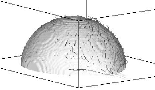
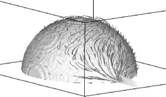
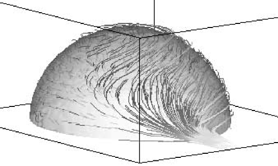
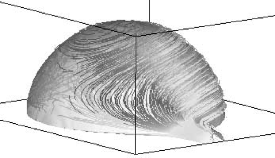
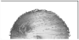
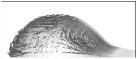
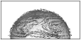
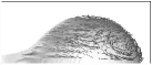
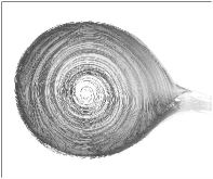
Figures 1(a)-(d) show the equi-density surface of the companion star and the streamlines starting from the equi-density surface; Fig. 1(a) depicts the equi-density surface of $\log_{10}\rho=-1$, (b) $-1.5$, (c) $-2$, and (d) $-2.5$. In order to draw the streamlines, we use the same integration time step. Therefore, the higher the density of gas, the shorter the streamlines as the velocity is lower. We observe that there are ascending motions of gas in the higher density region (deeper inside the star) and a remarkable circulating flow in the lower density region (surface region). The streamlines of lighter color have higher velocity than those of darker ones. As will be shown later, there is a high pressure around the north pole, and so we may call this circulatory flow the north pole circulatory flow or simply an H-eddy.

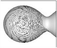
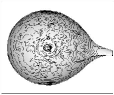
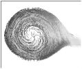
In order to see the surface flow more closely, Fig. 2 shows the equi-density surface ($\log_{10}\rho=-2$) of the companion star and the streamlines starting from the equi-density surface of $\log_{10}\rho=-2.5$ seen from various view angles. We confirm the presence of the H-eddy again. Gas in the H-eddy seems to drift gradually downward and its velocity increases with decreasing latitude. This phenomenon will be discussed later.

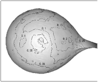
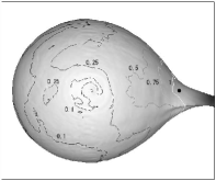
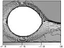
Figure 3 shows the iso-velocity lines plotted on the equi-density surface of $\log_{10}\rho=-2.5$ seen from the north pole. The numbers in the figure show the magnitude of the velocity (note that the velocity is normalized by $A\Omega$, where $A$ is the separation and $\Omega$ is the rotational frequency of the binary.)

In the L1 region, which is close to the L1 point, there is a strong low pressure due to the mass outflow through the L1 point. Because of the presence of the L1 low pressure, there is a circulatory flow, around the L1 point, rotating counter-clockwise, although this eddy does not form a complete circle for geometrical reasons. We call this flow the L1-eddy, although, strictly speaking, this is not a complete eddy.

The other remarkable feature is the presence of two eddies rotating counter-clockwise at the opposite side of the L1 point. These two eddies merge to form one larger eddy at different density levels. Since this region is close to the L2 point, we may call this eddy the L2 eddy. Since these H, L1 and L2 eddies are explained in terms of the astrostrophic wind (Lubow and Shu lub75 (1975)), the pressure distribution on the surface of the companion is important.

Figure 4: Isobaric lines plotted on the equi-potential surface seen from the north pole.

Figure 5: Isobaric lines plotted on the equi-density surface of $\log_{10}\rho=-2.5$ seen from the north pole.

3.2 High / low pressures on the companion surface

If there is no flow on the companion, the isobaric surface should coincide with the equi-potential surface as a result of the hydrostatic balance. In our case, the isobaric surface does not coincide with the equi-potential surface in an exact sense because of the presence of the surface flow. Fig. 4 shows the isobaric lines plotted on the equi-potential surface of the companion. This equi-potential surface nearly corresponds to the equi-density surface with $\log_{10}\rho=-2.5$ except near the L1 region, where high speed gas motion is present. Note that the isobaric lines on the companion surface have concentric patterns around the north pole.

As was described earlier, the flow pattern on the surface of the rotating (in the inertial frame) companion can be explained in terms of the astrostrophic wind, which is a counterpart of the geostrophic wind in the atmosphere of the Earth. If viscosity can be neglected, the direction of the flow is parallel to the isobaric lines of low/high pressure. In the present case of a counter-clockwise rotating binary system (as viewed from the north pole), the flow proceeds by keeping the high (low) pressure to the right (left) in the northern hemisphere. Therefore, the H-eddy circulates clockwise, while the L1 eddy and L2 eddy circulate in the counter-clockwise direction.

If the pressure is only a function of the density of gas, the gas is called barotropic. Otherwise, the gas is called baroclinic. In the case of $\gamma=1.01$, the gas is nearly iso-thermal, hence almost barotropic. In the other cases, the gas is baroclinic. In a barotropic gas, an isobaric surface must coincide with an equi-density surface. Fig. 5 shows the baroclinicity of the gas with $\gamma=5/3$, whose property is responsible for the generation of vorticity. This will be discussed later.

3.3 Ekman boundary layer

In the Earth’s atmosphere, an Ekman boundary layer exists close to the surface of the Earth, where (turbulent) viscosity cannot be neglected and where the direction of the flow deviates from that of a pure geostrophic wind. In low pressure regions, gas drifts inwards and eventually ascends near the centre of the low pressure regions (Pedlosky ped87 (1987)).

In our simulations, there is no (physical) viscosity assumed. Nevertheless, numerical viscosity arising from a truncation error acts as a kind of a turbulent viscosity, leading to gas drifting. This is the reason why the circulating flow about the north pole gradually migrates towards the equatorial region. In order to test the above consideration, we perform a calculation with the mesh size halved. In this case the magnitude of the (numerical) viscosity is expected to be $1/8$ of the coarser grid case. We find a similar flow pattern as before, although the circulating motion is tighter than before (see Figs. 6). The main characteristics of the flow pattern are not changed, though.

In the surface region of low-mass main-sequence stars, there is a convection zone, which provides the necessary turbulent viscosity. We may therefore expect that the present flow pattern is qualitatively correct.

It is however not trivial from our simulations to derive the exact value of our (numerical) viscosity. We can only make a very tentative guess that the typical Reynolds number in our simulations is probably of the order of 10 to 100. In a future work, we plan to solve this problem using the Navier-Stokes equation instead of the Euler ones, and using the molecular viscosity as a rough estimate of the turbulent viscosity which should be at play here.

In our case the inner boundary does not play the role of the surface of the Earth. The Ekman layer is present at the top of the atmosphere, a situation similar to a water vortex. Gas circulating around the high pressure region at the north pole migrates gradually towards the equator, switches to the counter-clockwise motion close to the L1 low pressure, and finally escapes from the companion towards the primary star. This flow pattern is important to understand the structure of the L1 stream to be discussed later.

(a)
(b)

Figure 6: (a) Calculation with mesh size $121{\times}101{\times}51$. (b) Calculation with mesh size $241{\times}201{\times}101$ at $t=12.56$.

3.4 Effect of $\gamma$

Until now we have shown the results for $\gamma=5/3$, corresponding to ionized hydrogen gas. In order to study the case of molecular hydrogen, we calculate the case $\gamma=7/5$. The results are essentially the same as for $\gamma=5/3$, so that we do not discuss them any further.

However, the results for $\gamma=1.01$ are very different from the cases of $\gamma=5/3$ and 7/5, and are essentially the same as that of Fujiwara et al. (fuj01 (2001)): there is no H eddy but the flow originating at the pole region migrates rather directly towards the equatorial region. More precisely, such a flow is rather weak, because the pressure on an equi-potential surface is rather uniform except in the region close to the L1 point. The L1 flow mainly originates from the region close to the L1 point. The case of $\gamma=1.2$ is intermediate to the above two extreme cases. We found the L2 eddy in this case.

We may explain the difference of the flow patterns between the cases of $\gamma=5/3,7/5$ and that of $\gamma=1.01$ in terms of the baroclinicity of the gas. Vorticity is generated by the term containing $\nabla\rho\times\nabla p$, which is identically zero for a barotropic gas (Pedlosky ped87 (1987)). Therefore, local vorticity of the gas in the case of $\gamma=1.01$ is almost zero everywhere. Moreover, the Taylor-Proudman theorem, which states that the horizontal velocity components $u$ and $v$ are independent of $z$, holds not only for an incompressible flow but also for a barotropic gas (Busse bus70 (1970); Pedlosky ped87 (1987)). Since $u$ and $v$ are almost zero on the inner boundary, they must also be small in the upper atmosphere. This problem, however, needs further investigation. We note that the cases of $\gamma=5/3$ and 7/5 are more appropriate to compare with (future) observations.

3.5 L1 region and L1 stream

Lubow and Shu (lub75 (1975)) paid lots of effort to solve the flow in the L1 region by their matched expansion technique. In this subsection we summarize our numerical results.

In order to make the influence of the outer boundary to the L1 stream small, we slightly expand the computational region of the $x$-component from $0.7$ to $0.9$ in this subsection. The primary star is still out of the computational region. Thus the L1 stream reaches the boundary at $x=0.9$ and escapes from the calculation region. In the present calculation no accretion disc is formed, and so there is no collision between the L1 stream and the accretion disc around the primary star.

Lubow and Shu (lub75 (1975)) predicted that the sonic point, where subsonic gas is accelerated to supersonic velocity, must occur close to the L1 point. Figure 7 shows the iso-Mach number lines on an equi-density surface and the numbers on the figure show the Mach number. It can be seen that the sonic line on the surface is certainly close to the L1 point.

Figure 7: Iso-Mach number lines on an equi-density surface with $\log_{10}\rho=-2.5$ seen from the north pole. The sonic line is close to the L1 point. The gray color shows the combined effect of the magnitude of the velocity and the lighting effect. The heavy black dot shows the position of the inner L1 point.

(a)

(b)

(c)

Figure 8: (a) Velocity vector in the orbital plane. Note that arrows are drawn only every four cells in each x and y direction. (b) Streamlines in the orbital plane with velocity magnitude contours. (c) Density contours with equi-density lines. The heavy black dot shows the position of the inner L1 point.

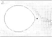
Figs. 8(a)-(c) show the velocity vectors, the streamlines, and the equi-density lines of the gas in the orbital plane, respectively. The flow pattern in the orbital plane near the L1 point shows some difference with the one depicted in Fig. 3 in Lubow and Shu (lub75 (1975)). They predicted that the streamlines of the lower portion of the L1 point turn back to the companion, while in our case all gas flow towards the primary compact component. There are two differences between thier assumptions and ours: 1) they assumed iso-thermal gas; 2) they start their calculation at the L1 point, where the gas is assumed to be at rest. The assumption 2) may be the main reason. We solve the whole region including both the L1 region and the surface layer of the companion. The gas at the L1 point is already supersonic as was described above.

From Fig. 8(b) we can measure the deflection angle $\theta_{s}$ of the L1 stream, which is the angle between the central flow line in the L1 stream and the $x-$axis. It is about -10 degrees. This angle was calculated to be about -20 degrees for the case of $q=1$ by Lubow and Shu (lub75 (1975)). In Fujiwara et al.’s result (fuj01 (2001)) this is about -15 degrees. This difference is also due to the difference in boundary conditions. Lubow and Shu assumed that the fluid element was at rest at the L1 point. The effect of the Coriolis force is measured by the Rossby number defined by $U/A\Omega$, where $U$ is a typical velocity of gas. The lower the initial velocity of the gas, the lower the Rossby number, the larger the Coriolis’ effect and, hence, the deflection angle.

In Fig. 8(c) we found that the atmosphere of the secondary is thicker in the leading hemisphere (negative $y$) than the trailing hemisphere. This can be easily explained by the direction of the Coriolis force, which acts to the right side of the flow direction in our system.

(a)
(b)

Figure 9: Density contours of the L1 stream at two cross sections: (a) $x=0.5$; (b) $x=0.65$. The horizontal axis is the $y$-axis ranging from -0.5 to 0.5. The vertical axis depicts the $z$-axis ranging from 0 to 0.5. Note the asymmetry of the density contour in the central part of the L1 stream.

Figure 10: Density profile along the $y$-axis on the orbital plane $z=0$ at various $x$ locations, ranging from $0.5$ to $0.8$.

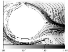
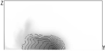
Because of this asymmetry of the atmosphere, the structure of the L1 stream is also asymmetric about the central flow line. In Figs. 9 we show the cross section of the L1 stream, which is bow shaped convex to the positive $y$ direction. We obtained a similar pattern in Fujiwara et al. (fuj01 (2001)), and this was explained by the interaction of the L1 stream and the circulating circum-disc flow on the orbital plane about the primary. In the present work we realize that this explanation is not correct. The bow shape of the L1 stream should be explained by the structure of the surface flow on the companion.

Lubow and Shu (lub75 (1975)) predicted a symmetric Gaussian density distribution at the centre of the stream as

$$\rho(r,\theta){\approx}\frac{C}{r}\exp[-Br^{2}(\theta-\theta_{s})^{2}],$$ (1)

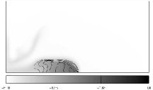
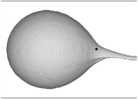
where $r$ is the distance from the L1 point in the scaled coordinate, $\theta_{s}$ is the angle of the stream centre from the line joining the centre of the two stars, and $C$, $B$ are the coefficients depending on the mass ratio. Fig. 10 shows that our density profile nearly has a Gaussian density distribution. The density at the centre of the stream obtained by them decreases as $r^{-1}$, while our result decreases as $r^{-0.8}$. Fig. 11 shows the equi-density surface of $\log{\rho}=-2.5$ of the companion star and the L1 stream.

Figure 11: Equi-density surface of $\log_{10}{\rho}=-2.5$ of the companion star and the L1 stream seen from the north pole. The heavy black dot shows the position of the inner L1 point.

Figure 12: Schematic diagram of the system of eddies: L1, H, and L2 show the low pressure near the L1 point, the high pressure around the north pole, and the low pressure at the opposite side of L1, respectively. An eddy rotates clockwise for H, and counterclockwise for L1 and L2.

4 Discussion

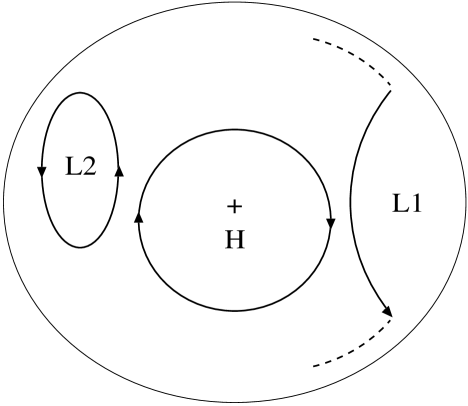
In our simulations, we obtained a system of eddies: the H eddy rotating clockwise, and counterclockwise rotating L1 and L2 eddies. We now discuss what we believe is the reason that this eddy system is formed (see Fig. 12).

If we consider a time sequence, the L1 low pressure is formed first, because of the mass loss through the L1 point. Since the gas near the equator does not feel much resistance in flowing towards the L1 point, the equatorial region becomes a low pressure zone, and a high pressure zone builds up at the north pole: the H eddy is thus formed.

The above explanation does not explain the appearance of the third eddy: the L2 eddy. This can be explained as follows. Consider a force exerted by an eddy on another eddy. The L1 eddy tries to convect the H eddy to negative $y$-direction, while the H eddy tries to convect the L1 eddy to negative $y$-direction as well. However, the L1 eddy must be fixed to the L1 region, so that the H eddy must drift to negative $y$-direction. The system is therefore not steady. In order to stabilize the eddy system, we need the third eddy, which tries to convect the H eddy to positive $y$-direction. The L2 eddy thus appears and evolves until the three eddy system is stabilized. The exact location and the strength of these eddies can be obtained only through numerical simulations.

It is interesting to note that Davey and Smith (dav92 (1992)) have found that the trailing hemisphere has stronger line absorption than the leading hemisphere in a dwarf nova (see also Dhillon and Watson dhi00 (2000)). This asymmetry can be naturally explained in terms of the H-eddy current, which convects heat due to irradiation to the leading hemisphere.

If this kind of astrostrophic wind conveys heat effectively from an irradiated hemisphere to the other, the unirradiated side of the companion becomes hotter than previously thought. Such an example may be observed in the 2000 outburst of the recurrent nova CI Aql because, in nova outbursts, a companion star should be strongly irradiated by a hot white dwarf. The inclination angle of the CI Aql orbit is about 80 degrees and the eclipse is almost total in the sense that the companion completely occults the bright accretion disc around the white dwarf (e.g., Hachisu & Kato 2001). In eclipse minima, therefore, we see only the unirradiated side of the companion. Hachisu, Kato and Schaefer (2002) showed that the eclipse minima of CI Aql in outburst is about 0.6 mag brighter than in quiescence and could reasonably reproduce the orbital light curve (folded by the orbital period) when the temperature of the unirradiated hemisphere is about 1000 K hotter than that in quiescence.

In the present study, we do not take into account such complex effects as (real) viscosity, magnetic fields, and irradiation from the accretion disc. Activities of magnetic fields on the companion surface would lead to star-spots, and the irradiation from the accretion disc would lead to an increase of the gas temperature of the companion. These effects might more or less change the surface flow patterns. The present study is a first step to examine the surface flow structure. Thus to study these phenomena is beyond the scope of the present paper, and is left for future work.

5 Summary

We performed numerical simulations of the surface flow on the companion star in a semi-detached binary system. The case with $\gamma=5/3$ was mainly studied, although the cases of $\gamma=7/5,1.2$ and 1.01 were also investigated. The results are summarized as follows:

1. We obtain an eddy configuration composed of an H-eddy, an L1-eddy, and an L2-eddy associated with high/low pressures. If there is no viscosity, the flow lines must be closed. The above eddies are explained in terms of the astrostrophic wind.

2. Some kind of viscosity (e.g., turbulent viscosity originating from a surface convection zone) would lead to a downward drifting motion. In our simulation the numerical viscosity acts as turbulent viscosity.

3. The sonic line on an equi-density surface occurs close to the L1 point.

4. The deflection angle of the L1 stream is about -10 to -15 degrees. This small angle is due to the larger fluid velocity at the L1 point.

5. The density distribution in the L1 stream is nearly symmetric about the central flow line. The cross section of the L1 stream is bow shaped convex to the positive $y$ direction. This is an intrinsic nature of the stream and is not caused by the interaction with the accretion disc gas.