Circular Polarization of Water Masers in the Circumstellar Envelopes of Late Type Stars

We present circular polarization measurements of circumstellar H₂O masers. The magnetic fields in circumstellar envelopes are generally examined by polarization observations of SiO and OH masers. SiO masers probe the high temperature and density regime close to the central star. OH masers are found at much lower densities and temperatures, generally much further out in the circumstellar envelope. The circular polarization detected in the (6₁₆–5₂₃) rotational transition of the H₂O maser can be attributed to Zeeman splitting in the intermediate temperature and density regime. The magnetic fields are derived using a general, LTE Zeeman analysis as well as a full radiative transfer method (non-LTE), which includes a treatment of all hyperfine components simultaneously as well as the effects of saturation and unequal populations of the magnetic substates. The differences and relevances of these interpretations are discussed extensively. We also address a non-Zeeman interpretation as the cause for the circular polarization, but this is found to be unlikely. We favor the non-LTE analysis. The H₂O masers are shown to be unsaturated, on the basis of their line widths and the lack of linear polarization. The field strengths are compared with previous detections of the magnetic field on the SiO and OH masers. Assuming a $r^{-2}$ dependence of the magnetic field on the distance to the star, similar to a solar-type magnetic field, our results seem to indicate that we are probing the highest density maser clumps at the inner edge of the H₂O maser region. This allows us to estimate the density of the clumps, and the extent of the H₂O maser region. We show that the magnetic pressure dominates the thermal pressure by a factor of $20$ or more. We also give an order of magnitude estimate of the magnetic field on the surface of the stars. In particular we discuss the differences between Supergiants and Mira variable stars.

Figure 1: Synthetic V-spectra for an external field of 50 mG and a line width of $\Delta v_{\rm L}=0.8$ km s^-1.

Figure 2: $B-P_{\rm V}$ relations. The solid lines represent the $F=7-6$ transition for different $\Delta v_{\rm L}$. The short- and long-dashed lines are the $F=6-5$ and the $F=5-4$ transition respectively. The dotted line is a typical best fitted model including all three hyperfine lines.

1 Introduction

A large majority of stars go through a period of high mass loss at the end of their evolution while climbing the asymptotic giant branch (AGB). This mass loss, of the order of $10^{-7}$ to $10^{-4}M_{\odot}/{\rm yr}$, is the main source for replenishing interstellar space with processed materials. Thus the mass loss mechanism is an important subject of study. In late type stars, this high mass loss produces a circumstellar envelope (CSE) in which several maser species can be found. These masers, especially SiO, H₂O and OH, are excellent tracers of the kinematics of the CSEs. The role of magnetic fields in the mass loss and formations of CSEs is still unclear. Polarization observations of circumstellar masers can reveal the strength and structure of the magnetic field throughout the CSE. Observations of SiO maser polarization have shown highly ordered magnetic fields close to the central star, at radii of 5-10 AU where the SiO maser emission occurs (e.g. Kemball & Diamond, 1997). The measured circular polarization indicates magnetic field strengths of $\approx 5-10$ G, when assuming a standard Zeeman interpretation. However, a non-Zeeman interpretation has been proposed by Wiebe & Watson (1998), which only requires fields of $\approx$ 30 mG. At much lower densities and temperatures and generally much further from the star, OH maser observations measure fields of $\approx 1$ mG (e.g. Szymczak & Cohen, 1997; Masheder et al., 1999) and there is little dispute of the Zeeman origin of the polarization. Until recently, no information on the magnetic fields at distances of a few hundred AU from the star was available. This is the region where the H₂O maser emission occurs. Because water is a non-paramagnetic molecule, determination of the magnetic field is significantly more difficult. The fields expected in the H₂O maser region are stronger than the fields measured for the OH masers; since they probably occur in gas that is a factor of $10-1000$ more dense and closer to the central star than the OH masers. So we expect fields of a few tens to a few hundred mG. For these fields the Zeeman splitting of H₂O is extremely small, only $\approx\leavevmode\nobreak\ 10^{-3}$ times the typical half-power width of the H₂O maser line ($\Delta\nu_{\rm L}\approx 30$ kHz). However, Vlemmings et al. 2001 (hereafter V01) have shown that in the presence of such magnetic fields the Zeeman splitting can be detected with high spectral resolution polarization observations. They presented the first results of circular polarization measurements of circumstellar H₂O masers on the masers around the supergiant star S Per. A ’basic’, LTE, Zeeman analysis was used to infer the magnetic field strength along the line of sight. This analysis did not include the interaction between the various hyperfine components of the 22 GHz H₂O transition. The observations confirmed the expected field strength, finding a field of $\approx 250$ mG. The method used in V01 was similar to the method used by Fiebig & Güsten (1989, hereafter FG) to analyze the circular polarization of strong interstellar H₂O maser features. Here we present observations for a sample of 4 stars. We discuss the data reduction path, and in addition to the FG method, we fit our observation to the theoretical, non-LTE, models of Nedoluha & Watson (1992), hereafter NW. These include hyperfine interaction as well as saturation effect. The non-Zeeman interpretations presented in Nedoluha & Watson (1990) and Wiebe & Watson (1998) are also discussed. Finally we present measurements of the linear polarization.

2 Theoretical Framework

2.1 Standard Zeeman interpretation

Figure 3: Fractional circular polarization in units of $0.1\%$. The solid line is the total intensity Stokes $I$, the long-dashed line is Stokes V. Left has $v_{\rm thermal}=0.6$ km/s, right has $1.0$ km/s. The models are labeled for emerging brightness temperature $T_{\rm b}\Delta\Omega=10^{11},10^{10}$ and $10^{8}$ from top to bottom. The solid vertical line indicates the peak and the short dashed lines the FWHM of the profile.

Figure 4: Linear polarization for $\theta=75^{\circ}$. The dashed line is linear polarization is given in units of $10\%$. Labelling is similar as Fig. 3

2.1.1 Basic LTE analysis

Our first treatment of the standard Zeeman interpretation closely follows the analysis performed in FG and is more thoroughly discussed in both V01 and FG. This is a standard method that assumes LTE. Thus, the narrowing and rebroadening of the lines as a result of maser saturation are not reproduced. We have included the possibility of multiple masing hyperfine components, assuming the $F=7-6$ hyperfine component to be dominant. Each hyperfine component will split into 3 groups of lines ($\sigma^{+},\sigma^{-}$ and $\pi$). For a magnetic field B parallel to the line of sight, the Zeeman pattern consists of the two circular polarized $\sigma$ components only. The right- and left-handed (RR and LL) spectra, corresponding to the $\sigma^{\pm}$ components will only be slightly shifted against each other. This corresponds to a characteristic frequency shift of the order of $\Delta\nu_{\rm Z}\approx 10^{3}$ Hz$\cdot B_{\rm[Gauss]}$. As a result, the observed V-spectrum (RR-LL) will be a sine-shaped function, corresponding to the derivative $I^{\prime}$ of the total power spectrum. The amplitude of this function depends on the maser line width, the magnetic field strength, and on which hyperfine components actually contribute to the maser. By calculating synthetic V-spectra we find the following relation for the percentage of circular polarization:

$$P_{\rm V} = (V_{\rm max}-V_{\rm min})/I_{\rm max}$$ (1)

$$= 2\cdot A_{\rm F-F^{\prime}}\cdot B_{\rm[Gauss]}\rm{cos}\theta/\Delta v_{\rm L}[\rm{km\leavevmode\nobreak\ s}^{-1}].$$

Here $V_{\rm max}$ and $V_{\rm min}$ are the maximum and minimum of the synthetic V-spectrum fitted to the observations. $\Delta v_{\rm L}$ is the full width half-maximum (FWHM) of the total power spectrum, and $I_{\rm max}$ is the peak flux of the maser feature. $B$ is the magnetic field strength and $\theta$ the angle between the magnetic field lines and the line of sight. The $A_{\rm F-F^{\prime}}$ coefficient depends on the masing hyperfine components. The $A_{\rm F-F^{\prime}}$ coefficients have been determined by calculating $P_{\rm V}$ from synthetic V-spectra, determined for a series of magnetic field strengths $B$, and for the different hyperfine components. Some examples of synthetic V-spectra for the three hyperfine lines are shown in Fig. 1. The $B-P_{\rm V}$ relation is shown in Fig. 2 for different hyperfine components and line widths. For the different hyperfine transitions separately, FG find $A_{\rm F-F^{\prime}}=0.013,0.08$ and $0.01$ for the $7-6,6-5$ and $5-4$ transitions respectively. For the fitted combinations of hyperfine components we generally find $A_{\rm F-F^{\prime}}\approx 0.011$.

2.1.2 Full radiative transfer, non-LTE analysis

Figure 5: a) Spectral line width versus emerging brightness temperature $T_{\rm b}\Delta\Omega$. The solid, dotted and dashed lines have $\Delta v_{\rm thermal}=0.6,1.0$ and $2.0$ km/s respectively. b) $P_{\rm V}$ versus $T_{\rm b}\Delta\Omega$. Labeling is similar to a), thin lines have $\theta=0^{\circ}$, thick lines correspond to $\theta=75^{\circ}$.

The transfer equations for the polarized radiation of the 22 GHz H₂O masers in the presence of a magnetic field were solved in NW. We have redone the calculations to fit the theoretical total intensity and circular polarization spectra to our observations. They were performed for the combination of the three strongest hyperfine components which have previously been verified to make the only significant contribution (Deguchi & Watson, 1986; Nedoluha & Watson, 1991). We solve a related set of 99 equations of state for all the magnetic substates of the relevant hyperfine components.

The goal of NW was to asses the validity of Eq. 1 when specific effects of maser radiation are included in the analysis. The LTE treatment described above for example, does not include: narrowing and rebroadening of the maser line with increasing optical depth, hyperfine interaction, unequal populations of the magnetic substates and the generation of circular polarization due to changes in direction of the linear polarization. To solve the equations of state, some assumptions have been made. The Zeeman frequency shift $g\Omega$, is assumed to be much greater than the rate for stimulated emission $R$, decay rate $\Gamma$ and cross-relaxation rate $\Gamma_{\nu}$. In this regime the off-diagonal elements of the density matrix which describes the molecular states are negligible, which greatly simplifies the calculations. The maser is assumed to propagate nearly one-dimensionally. Additionally, the pumping has a Maxwellian velocity dependence and is the same for all magnetic substates.

For expected magnetic fields of $\approx$ 100 mG the values of $g\Omega$ for the stronger hyperfine transitions are about 1000 ${\rm s}^{-1}$. The rate for stimulated emission can be estimated by:

$$R\simeq AkT_{\rm b}\Delta\Omega/4\pi\hbar\omega$$ (2)

Here $T_{\rm b}$ is the brightness temperature, $\Delta\Omega$ the beaming solid angle for the maser radiation and $A$ the Einstein coefficient. For $T_{\rm b}\Delta\Omega\leavevmode\nobreak\ =\leavevmode\nobreak\ 10^{12}$, $R\approx 100\leavevmode\nobreak\ {\rm s}^{-1}$. Thus $g\Omega\gg R$, required for ignoring the off-diagonal elements of the density matrix, is satisfied for most of the relevant brightness regime, up to $T_{\rm b}\Delta\Omega=10^{12}$. For higher brightness temperatures the results for $\theta\neq 0^{\circ}$ may be unreliable. For $\theta=0^{\circ}$ the off-diagonal elements are not present, thus the results are reliable up to the highest values of $T_{\rm b}\Delta\Omega$.

Detailed calculations of the cross-relaxation rate ($\Gamma_{\nu}$), which is expected to be considerably larger than the decay rate ($\Gamma$), give $\Gamma_{\nu}=2\leavevmode\nobreak\ {\rm s}^{-1}$ at temperatures of 400 K (Anderson & Watson, 1993). So $g\Omega\gg\Gamma_{\nu}\gg\Gamma$ is satisfied as well. The calculations here use $(\Gamma+\Gamma_{\nu})=1\leavevmode\nobreak\ {\rm s}^{-1}$, but NW have shown that the resulting intensities scale with the decay rate and the cross-relaxation rate as $[{\rm flux}/(\Gamma+\Gamma_{\nu})]$.

To perform the numerical calculations, we had to chose the strength of the radiation incident onto the masing region. The calculations presented here are based on a radiation of $T_{\rm b}\Delta\Omega=0.1$ K sr. This continuum radiation is taken to be unpolarized. It was verified in NW that the results are insensitive to the chosen value, and we have confirmed this result.

In contrast to the LTE analysis presented above, the results from the non-LTE transfer treatment are V-spectra which are not anti-symmetric. This can be seen comparing the non-LTE spectra in Fig. 3 to the synthetic LTE spectra in Fig. 1. The spectra are not proportional to the derivative of the total power intensity profile, I’, as used before, due to the blending of hyperfine lines with different $g\Omega$.

Fig. 3 also shows that for high $T_{\rm b}\Delta\Omega$, the total intensity spectra are increasingly less Gaussian in shape. The line shape thus enables us to estimate the saturation level of the maser. The model with $T_{\rm b}\Delta\Omega=10^{8}$ corresponds to a completely unsaturated maser. The models with $T_{\rm b}\Delta\Omega=10^{10}$ and $10^{11}$ correspond to slightly and fully saturated masers respectively. The non-LTE analysis also produces linear polarization for $\theta\neq 0^{\circ}$. Stokes $Q$ is shown in Fig. 4, which indicates that for $\theta=75^{\circ}$, linear polarization of up to $\approx 10\%$ is observed for $T_{\rm b}\Delta\Omega\approx 10^{11}$. NW show that for slightly saturated masers, linear polarization of a few percent should be observed when $\theta>15^{\circ}$.

The calculations have been performed for several different values of intrinsic thermal width ($v_{\rm thermal}$). This is the FWHM of the Maxwellian distribution of particle velocities. Assuming a kinetic temperature of $T$ K, $v_{\rm thermal}\approx 0.5(T/100)^{1/2}$ (NW).

The variation of line width with brightness temperature is shown in Fig. 5a for different values of $v_{\rm thermal}$. This relation does not depend on the angle $\theta$. We see a gradual narrowing of the maser line, and rebroadening occurs when the maser starts to become saturated, at $T_{\rm b}\Delta\Omega\approx 10^{10}$. The relation between the fractional circular polarization $P_{\rm V}$ and $T_{\rm b}$ does depend on $\theta$ and is shown for different values of $\theta$ and $v_{\rm thermal}$ in Fig.5b. The fractional circular polarization decreases with increasing maser intensity as the total intensity grows faster than the circular polarization. Both these relation scale with $[{\rm flux}/(\Gamma+\Gamma_{\nu})]$, similar to the intensity profiles.

Figure 6: $A_{F-F^{\prime}}$ coefficients as a function of $T_{\rm b}\Delta\Omega$. The lower panel shows $\theta=0^{\circ}$, the upper panel $\theta=75^{\circ}$. The solid, dotted and dashed lines correspond to $\Delta v_{\rm thermal}=0.6,1.0$ and $2.0$ km/s respectively.

From these relations we can now determine the coefficients $A_{\rm F-F^{\prime}}$ from Eq.1 which are shown in Fig.6. As can be seen, $A_{\rm F-F^{\prime}}$ depends strongly on $v_{\rm thermal}$. For small angles $\theta$ there is no strong dependence on $T_{\rm b}$, but for $\theta>45^{\circ}$, $A_{\rm F-F^{\prime}}$ can change by over a factor of $6$ for high $T_{\rm b}$. Neufeld & Melnick (1990) argue that the low values of $v_{\rm thermal}$ can be eliminated, on the basis of realistic H₂O maser pumping schemes. Values as high as $v_{\rm thermal}\approx 2.0$ km/s indicate temperatures of more than $1000$ K, which is expected to be too high according to the same analysis by Neufeld & Melnick. From linewidth analysis we conclude that $v_{\rm thermal}\approx 1.0$ km/s is the most realistic estimate, which yields $A_{\rm F-F^{\prime}}\approx 0.018$. This value does not decrease by more than $10\leavevmode\nobreak\ \%$ if we take $v_{\rm thermal}\approx 1.5$ corresponding to the upper temperature limit of $1000$ K.

Figure 7: $\theta$-dependence of Eq. 1 for increasing emerging brightness temperature $T_{\rm b}\Delta\Omega$. The lines for $T_{\rm b}\Delta\Omega=10^{7}$ and $10^{8}$ coincide and are the same as the lines for lower brightness temperatures.

The effect of the angle $\theta$ has recently been examined by Watson & Wyld (2001) for the general case of a transition with low angular momentum (J=1-0 and J=2-1). They conclude that for masers that are at least partially saturated the circular polarization does not decrease with increasing $\theta$ until the magnetic field and the propagation direction are nearly perpendicular. We have performed similar calculations for the specific 22 GHz H₂O maser transitions and the results are shown in Fig. 7, which confirm for transitions with higher angular momentum, the analysis of Watson & Wyld.

2.2 Non-Zeeman interpretation

Circular polarization can also occur due to the change of the axis of symmetry for the molecular quantum states from parallel to the magnetic field, to parallel to the direction of propagation. When $g\Omega\gg R$, the direction of the magnetic field is the axis of symmetry. When $g\Omega\ll R$, the molecules interact more strongly with the radiation than with the magnetic field, and the direction of propagation is the axis of symmetry. Initially $g\Omega\gg R$, but as the maser propagates through the medium and becomes more intense, $g\Omega\ll R$ could possibly be satisfied. This was discussed by Nedoluha & Watson (1990) and was shown to lead to an overestimation of the magnetic field by up to a factor of 1000. However, the study in NW, and the line width observed here, show that the effect described above is unimportant for H₂O masers. The line widths show that in almost all cases $g\Omega\gg R$ is satisfied.

Wiebe & Watson (1998) have shown that the propagation of linear polarization can also result in circular polarization. For linear polarizations of $\approx 10\%$, the resulting circular polarization is of the same order of magnitude as the polarization due to the regular Zeeman interpretation, while magnetic fields could again be a factor of 1000 less. Below we indicate that also this non-Zeeman interpretation is unlikely due to the lack of linear polarization.

2.3 Fitting Method

2.3.1 LTE Zeeman

In the case of the LTE Zeeman models we first fit a combination of the 3 strongest hyperfine components to the total power spectrum. From this we get the line width $\Delta v_{\rm L}$ of the maser feature and the contribution to the line of the hyperfine components. For this combination we calculate a synthetic V-spectrum, such as shown in Fig. 1 for the separate hyperfine components. The synthetic spectrum is then fitted to the circular polarization spectrum. As our observations in V01 have shown that the observed V-spectrum can be narrower than the synthetic V-spectrum, we also allow for the narrowing of our synthetic spectra in the fit. Furthermore we need to remove the scaled down replicas of the total intensity. We fit the following function:

$$V_{\rm obs}(\Delta v)=a_{1}\cdot V^{*}(a_{2}\cdot\Delta v)+a_{3}\cdot I(\Delta v)$$ (3)

Here $\Delta v$ is the velocity in [km/s] measured from the peak of the total intensity, $V^{*}$ is the synthetic spectrum $V_{\rm synth}$. We fit for the parameters $a_{1}$, $a_{2}$ and $a_{3}$. The parameter $a_{1}$ controls the amplitude of the V-spectrum, while $a_{2}$ determines the amount of narrowing of the observed spectra with respect to the model spectra. Finally, the removal of the scaled down total intensity profile is determined by $a_{3}$. The amplitude $a_{1}$ of the best fitted model determines $V_{\rm min}$ and $V_{\rm max}$. Together with the peak intensity of the maser feature this gives $P_{\rm V}$. With the previously determined line width $\Delta v_{\rm L}$ we calculate $B_{||}$ using Eq. 1.

2.3.2 Non-LTE

For the non-LTE case, we fit out models to both total intensity and circular polarization simultaneously. We use Eq. 3 with $V^{*}=V_{\rm model}$. Because the non-LTE models are already intrinsically more narrow, we first fix the width of the V-spectrum by setting $a_{2}=1.0$ and only fitting $a_{1}$ and $a_{3}$. We have chosen to fit models with $v_{\rm thermal}=0.8$ and $1.0$ km/s, as the line widths of the maser features indicate that much higher intrinsic thermal widths are unlikely. We find that in some cases the circular polarization spectrum is still narrower than the model spectrum. For these features we allow for narrowing by releasing $a_{2}$. The combined fitting determines the circular polarization percentage $P_{\rm V}$ and the line width $\Delta v_{\rm L}$. The coefficient $A_{\rm F-F^{\prime}}$ is specifically determined for the best fitted model. Using this Eq. 1 again gives $B_{||}$.

3 Observations

Table 1: Star Sample

Name	Type	RA (J2000)	Dec (J2000)	Distance	Period	Vrad	Peak flux
		(${}^{h}\leavevmode\nobreak\ {}^{m}\leavevmode\nobreak\ {}^{s}$)	(${}^{\circ}\leavevmode\nobreak\ {{}^{\prime}}\leavevmode\nobreak\ {"}$)	(pc)	(days)	(km/s)	(Jy)
S Per	Supergiant	02 22 51.72	+58 35 11.4	1610a	822	-38.1	76.1
U Her	Mira	16 25 47.4713	+18 53 32.867	189b	406	-14.5	12.5
NML Cyg	Supergiant	20 46 25.7	+40 06 56	1220c	940	0.0	48.2
VY CMa	Supergiant	07 22 58.3315	-25 46 03.174	1500d	2000	22.0	244.1
a Hipparcos,bvan Langevelde et al. (2000), cDance et al.(2001) , dLada & Reid (1978)

The observations were performed at the NRAO Very Long baseline Array (VLBA) on December 13th 1998. At the frequency of the $6_{16}-5_{23}$ rotational transition of H₂O, 22.235 GHz, the average beam width is $\approx 0.5\times 0.5$ mas. This allows us to resolve the different H₂O maser features in the CSE. The data were correlated twice, once with modest ($7.8$ kHz $=0.1$ km s^-1) spectral resolution, which enabled us to generate all 4 polarization combinations (RR, LL, RL and LR). The second correlator run was performed with high spectral resolution ($1.95$ kHz $=0.027$ km s^-1), necessary to detect the circular polarization signature of the H₂O Zeeman splitting, and therefore only contained the two polarization combinations RR and LL. We have performed 6 hours of observations per source-calibrator pair. The calibrator was observed for $1\leavevmode\nobreak\ 1/2$ hours in a number of scans equally distributed over the 6 hours. We used 2 filters (IFs) of 1 MHz width, which were overlapped to get a velocity coverage of $\approx 22$ km/s. This covers most of the velocity range of the H₂O maser.

3.1 Calibration of the Data

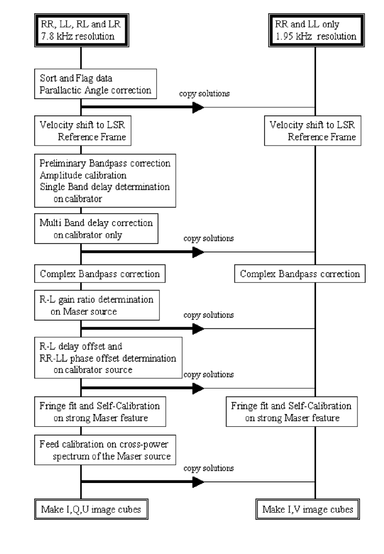
Figure 8: The schematic data reduction path for our spectral line polarization data

The data analysis followed the method of Kemball, Diamond & Cotton (1995). The reduction path, shown in Fig. 8, was performed in the AIPS data reduction package. The first standard calibration steps were performed on the data-set with modest spectral resolution. We used the system temperature measurements provided with the data to perform the amplitude calibration for both the calibrators and the sources. Parallactic angle correction, flagging and single- and multi-band delay calibration were all done regularly on the calibrators observed with each source. During 1/3 of the observation time, the first IF suffered strong interference, which forced us to flag several of the frequency channels ($\approx 0.1$ MHz) in addition to the normal flagging. Also, for most of the observations IF 1 of the Los Alamos (LA) antenna was unusable. The solutions obtained at these calibration steps were copied and applied to the high spectral resolution data set. The complex bandpasses were then determined for both data-sets separately. Additional calibration steps were needed for accurate processing of polarization data. The gain ratio between the R- (right-) and L- (left-) hand polarizations was determined using the auto-correlation data of the reference antenna on a short scan of the maser source. This step contains the critical assumption of equal flux for the R- and L-handed circular polarizations. As a result the circular polarization spectra are forced to be anti-symmetric, as discussed below. Later, during the analysis of the circular polarization spectra, we still have to correct for small replicas of the total power profiles due to remaining small gain differences. After the gain calibration, we used the calibrators to determine the R-L delay offset and the RR-LL phase offset. The delay offset is expected to be stable over the duration of the observation (Brown et al. 1989) and can be determined from a single continuum scan in which the cross-hand fringes RL and LR are well detected. The RR-LL phase offset varies over the observation and are determined from calibrators which are assumed to show no circular polarization. The solutions were again copied from the modest resolution date and applied to the high resolution data. Then fringe fitting and self-calibration for the two separate data-sets were performed on a strong maser feature. Finally, corrections were made for the instrumental feed polarization using a range of frequency channels on the maser source, in which the expected linear polarization or the frequency averaged sum of the linear polarization is low. After the solutions were applied to both data sets image cubes could be created.

3.2 Sample

We observed 4 late type stars, the supergiants S Per, VY CMa and NML Cyg and the Mira variable star U Her. They are listed in Table. 1 with type, position, distance, period and velocity. The sources were selected on the basis of 2 criteria; strong H₂O masers and previous SiO and OH maser polarization observations. The peak fluxes measured in these observations are also shown in Table. 1. On the total intensity channel maps with high spectral resolution, the noise is dominated by dynamic range effects and lies between $\approx 0.08-0.3$ Jy. On the circular polarization maps we have noise of $\approx 0.01-0.03$ Jy.

The circular polarization of the SiO masers around VY CMa has previously been observed with a single dish by Barvainis et al. (1987). They find circular polarization of $6.5\leavevmode\nobreak\ \%$, indicating a field strength of $B_{\rm SiO}\approx 65$ G. Observations of the 1612 MHz main line OH maser by Cohen et al. (1987) give $B_{\rm OH}\approx 2$ mG. Smith et al.(2001) concluded from ground based and Hubble Space Telescope optical observation, that high magnetic fields of at least $1$ G are necessary to explain the outflow of matter observed in VY CMa. Cohen et al. also detected fields of $\approx 2$ mG on the 1612 MHz OH masers around NML Cyg, while Masheder et al. (1999) estimated a field of $\approx 1$ mG on the OH masers around S Per. On U Her, Palen & Fix (2000) observed pairs of R- and L-polarized maser features, for the 1665 and 1667 MHz OH masers. Although not many of these Zeeman pairs were found they estimate a magnetic field of $B_{\rm OH}\approx 1$ mG.

4 Results

Figure 9: (left) Total intensity image of the H₂O maser features around S Per (right). Total power (I) and V-spectra for selected maser features of S Per. The bottom panel shows the best fitting synthetic V-spectrum produced by the standard Zeeman interpretation (dashed line). The middle panel shows the best non-LTE model fit (dotted line). The corresponding total power fits are shown in the top panel. The V-spectra in the lower two panels are adjusted by removing a scaled down version of the total power spectrum determined in the fit by the $a_{3}$ parameter in Eq.3, which is different for the LTE and non-LTE fits. The solid vertical lines show the expected position of minimum and maximum of the sine-shaped function in the general Zeeman case.

Table 2: Results

Name	Feature	Flux (I) (Jy)	$V_{\rm rad}{\rm(km/s)}$	$\Delta v_{\rm L}\leavevmode\nobreak\ {\rm(km/s)}$	P${}_{\rm V}\leavevmode\nobreak\ (\cdot 10^{-3})$	B ${\rm cos}\theta\leavevmode\nobreak\ {\rm(mG)}$ LTE	B ${\rm cos}\theta\leavevmode\nobreak\ {\rm(mG)}$ non-LTE
S Per	a	76.1	-27.2	0.88			$<$ 26
	b	57.7	-30.9	0.77	6.20	-207$\pm$30	-132$\pm$18
	c	11.4	-33.9	1.21			$<$ 254
	d	34.7	-37.1	0.54	5.62	-140$\pm$32	-77$\pm$17
	e	29.7	-28.9	0.61			$<$ 41
	f	35.6	-40.1	0.53			$<$ 33
	g	15.4	-30.4	0.92			$<$ 125
	h	14.9	-34.2	0.48			$<$ 75
	i	12.9	-39.3	0.69			$<$ 121
	j∗	26.6	-39.2	0.64	2.41	-156$\pm$47	-68$\pm$35
	k	14.2	-27.2	0.51			$<$ 72
	l	10.0	-23.2	0.44			$<$ 110
VY CMa	a∗	244.1	10.8	0.66	3.70	-116$\pm$21	-151$\pm$21
	b	155.5	10.6	0.67	5.64	182$\pm$30	99$\pm$15
	c	115.2	12.9	0.74	2.73	85$\pm$18	112$\pm$19
	d	47.9	13.7	0.83	3.24	129$\pm$31	81$\pm$16
	e	17.8	15.0	0.94	4.10	164$\pm$66	166$\pm$55
	f	58.5	18.3	0.80			$<$ 25
	g	25.3	27.1	0.88			$<$ 55
	h	43.1	28.8	0.61			$<$ 25
	i	65.6	25.2	0.79	2.23	83$\pm$25	48$\pm$14
	j	126.2	24.6	0.60	4.66	133$\pm$26	85$\pm$12
NML Cyg	a∗	48.2	-21.2	0.66	5.9	215$\pm$37	118$\pm$15
	b	10.5	-20.4	0.40	13.8	234$\pm$63	221$\pm$41
	c	5.42	-20.2	0.54	19.2	492$\pm$133	336$\pm$67
	d	3.66	-20.0	0.54	21.6	553$\pm$220	428$\pm$149
U Her	a	12.20	-17.8	0.75	27.5	858$\pm$161	605$\pm$83
	b	2.91	-17.6	0.50	126.1	2434$\pm$505	1487$\pm$231
	c	1.16	-17.6	0.73			$<$ 803
	d∗	2.46	-19.2	0.47	49.6	1181$\pm$297	552$\pm$114
	e∗	2.07	-19.2	0.51	41.1	980 $\pm$298	726$\pm$189
	f	1.36	-19.3	0.51			$<$ 337
∗ See text

We have examined the strongest H₂O maser features around the 4 stars observed. The results are shown in Table 2 for features with fluxes up to $10\%$ of the brightest maser spots. Some selected spectra are shown with fits of the LTE Zeeman models and the non-LTE models. When using the non-LTE models, fits with $v_{\rm thermal}=1.0$ km/s generally are best. As expected the splitting is small and the circular polarization is generally not more than $0.5-1.0\%$. Magnetic field strengths obtained using the LTE Zeeman models are given in column 7 while the results obtained using the non-LTE models are shown in column 8. The features that show less than a $3\sigma$ circular polarization signal are considered non-detections. For these we have determined (absolute) upper limits using the $A_{\rm F-F^{\prime}}$ coefficients obtained using the NW radiative transfer models. When using the LTE Zeeman analysis the limits increase by a factor of $\approx 1.4$.

Features labeled ^∗ have V-spectra that did not allow accurate fitting, possibly due to blending effects. They do show circular polarization above the $3\sigma$ level, although generally only slightly more. For these we have used $V_{\rm min}$ and $V_{\rm max}$ to estimate the magnetic field strength, and we assumed the best estimate for the coefficient $A_{\rm F-F^{\prime}}=0.018$. The errors are the formal $1\sigma$ errors.

We have not been able to detect linear polarization in any of the 4 sources. This gives upper limits to the fractional linear polarization of $\approx 1\%$ for the weakest features down to $\approx 0.01\%$ for the strongest.

4.1 S Per

Fig. 9 shows the total intensity map of the H₂O maser features around S Per, in which we can identify most of the features detected in earlier observations(Diamond et al. 1987; Marvel 1997). Positions are shown relative to the feature labeled S Per b, discussed in more detail in V01. Circular polarization between $0.2-0.7\%$ has been detected in 3 of the brightest features after a careful reexamination of the data. This has also resulted in a slightly lower magnetic field strength value for S Per b than the one presented in V01 after optimizing the fitting routines. The figure also shows the total power and circular polarization spectra for 2 of the features, with fits for both the LTE and non-LTE Zeeman models. The velocity labeling has changed from V01 to correspond to the convention used by NW. We find the magnetic field pointing away from us on all features. From these results we estimate the magnetic field in the H₂O maser region around S Per to be $\approx$ 200 mG using the LTE Zeeman analysis or $\approx$ 150 mG using the non-LTE models.

The maximum radius of the H₂O maser region was determined to be $\approx 60$ mas by Diamond et al.(1987), corresponding to $\approx 100$ AU. They conclude for a thick shell model that the inner radius of the water maser shell is $\approx 30$ mas, while the outer radius is $\approx 70$ mas. For comparison, the OH maser shell extent was determined by them to be $80\times 30$ mas, using MERLIN observations.

4.2 VY CMa

Figure 10: Similar to Fig. 9 for VY CMa

The total intensity map of the H₂O masers around VY CMa is shown in Fig. 10. Circular polarization has been detected on 7 out of 10 of the brightest maser features down to $P_{\rm V}\approx 0.2\%$. Similar to the values found for S Per we find a magnetic field of $\approx 200$ mG using the LTE Zeeman analysis or $\approx 175$ mG using the NW models. The magnetic field points toward us for most of the sources. VY CMa a suffers from blending with nearby maser spots which made accurate fitting impossible, this can also explain the change of sign.

Diamond et al.(1987) give the radius of the H₂O maser region for VY CMa to be $\approx 150$ mas, corresponding to $\approx 220$ AU. The 1612 MHz OH maser radius is shown to be $\approx 2400$ AU in observations by Reid et al.(1981).

4.3 NML Cyg

Figure 11: Similar to Fig. 9 for NML Cyg

We have only been able to detect a few H₂O maser features around NML Cyg, which are shown in Fig. 11. We find circular polarization from $0.6-2\%$. The spectra for NML Cyg b and c are shown in the same Figure. The V-spectrum for NML Cyg a is shown in Fig. 12. The circular polarization spectrum seems to indicate that this features actually consists of 2 heavily blended features of $\approx 30$ Jy. The magnetic field strength on this feature has been estimated using this simple model. Both the interpretations indicate the magnetic field strength to be $\approx 500$ mG, higher than for both S Per and VY CMa.

The H₂O maser region extent is $\approx 195$ mas, corresponding to $\approx 240$ AU (Johnston et al. 1985). Diamond et al.(1984) give for the 1612 MHz OH masers a maximum extent of $\approx 3-5$ arcsec.

Figure 12: Total power (I) and circular polarization (V) of NML Cyg a. Dotted and dashed lines are the model of two slightly shifted spatially blended maser features.

4.4 U Her

Figure 13: Similar to Fig. 9 for U Her

The total intensity map for the H₂O masers around U Her is shown in Fig. 13. U Her is the only Mira variable star in our sample and shows significantly weaker H₂O masers. However as seen in the figure, we do detect circular polarization of up to $\approx 10\%$. The field strength in the H₂O maser region of U Her is higher than those observed for the supergiant stars in our sample. We find strengths of $\approx 2.5$ G using the LTE Zeeman analysis or $\approx 1.5$ G using the non-LTE models. While the features U Her a and b show a clear sine-shaped V-spectrum, the features d and e have circular polarization signals only slightly outside the $3\sigma$ detection limit. This made fitting actual profiles impossible for those features.

The size of the H₂O maser region is found to be $\approx 350\times 200$ mas (Bowers et al. 1989), which at 189 pc distance corresponds to $\approx 65\times 40$ AU. Chapman et al. (1994) find for the OH maser extent of U Her of $800\times 900$ mas, $\approx 150\times 170$ AU.

5 Discussion

5.1 Interpretation of the Polarization Results

The observations show magnetic fields in the range from $\approx 150$ mG to $\approx 1.5$ G in the H₂O maser regions of our sample of stars. The exact field strength depends on the interpretation used. Here we have used the LTE Zeeman analysis presented in FG and V01, as well as a non-LTE model presented by NW. Generally, the results using the NW method give fields approximately $2/3$ of the LTE Zeeman method. As shown above, the non-LTE models do not typically produce anti-symmetric shapes for the circular polarization spectra. However, the anti-symmetric shapes observed are a necessary result of the data treatment, when it is assumed that the R- and L-polarization profiles are similar and when the scaled down replica of the total power spectrum is removed. We can thus fit both interpretations to the data by leaving the amplitude of the total power replicas as a free parameter as described in Section 2.3. As a consequence, we are unable to directly distinguish between the different interpretations on the basis of the anti-symmetry of the V-spectra.

The shape and line widths of the total intensity spectra of the different maser features indicate that for all stars the masers are unsaturated or only slightly saturated. As a result, even for the non-LTE case, we do not expect significant deviations from anti-symmetry. The line widths also indicate that $v_{\rm thermal}\approx 1.0$ km/s is indeed the best estimate for the thermal line width. In the cases where we could not perform good fits to the spectra, we have thus used $A_{\rm F-F^{\prime}}=0.018$ as the best estimate. Since the masers are thought to be unsaturated the circular polarization decreases linearly with ${\rm cos}\leavevmode\nobreak\ \theta$, as shown in Fig. 7.

An important motivation for using the non-LTE approach, is the fact that the circular polarization spectra show narrowing that is not expected in the LTE case, as discussed in V0. The observed spectra are not directly proportional to $I^{\prime}$, as the minimum and maximum are closer together than predicted. We can express this narrowing as $f_{\rm n}=\Delta v_{\rm L}/\Delta v_{\rm mm}$, where $\Delta v_{\rm L}$ is the FWHM of the maser feature and $\Delta v_{\rm mm}$ the separation between the minimum and maximum of the V-spectrum. $\Delta v_{\rm mm}$ is determined after the spectrum is forced to be anti-symmetric by fitting the scaled down total power spectrum. In our spectra we find on average $f_{\rm n}\approx 0.64$, but sometimes as low as $0.45$, which cannot be explained by LTE Zeeman models. In that case, when $V\propto I^{\prime}$, we find $f_{\rm n}\approx 0.85$. The non-LTE models partly explains this narrowing. As a result of the narrowing and rebroadening of the maser lines and of the hyperfine interaction, $f_{\rm n}$ depends on the maser brightness as shown in Fig. 14. The narrowing fraction decreases to $\approx 0.6$ in the case of highly saturated masers. However, as discussed above, the maser are indicated to be mostly unsaturated and thus the reason for the narrowing is still not completely clear. We have performed some tests using bi-directional masers. As seen in Fig. 14, these show more narrowing over the entire range, while the limit for the saturated masers is similar to the uni-directional masers. Thus, although the predicted narrowing fraction is still higher than observed, this is probably due to the assumption of linear masers in the models. Aside from the narrowing of the circular polarization profiles for bi-directional masers, the resulting $A_{\rm F-F^{\prime}}$ coefficients and corresponding magnetic fields do not change. We have used the uni-directional models for the fits, since the computation time increased considerably when calculating the bi-directional case.

Figure 14: Fractional narrowing of the non-LTE models as a function of emerging brightness temperature. The solid line indicates the uni-directional maser, the dotted line is the bi-directional maser. Both models have $v_{\rm thermal}=1.0$ km/s. The long-dashed line is the theoretical value for the LTE Zeeman analysis, while the dashed-dotted line is our measured average narrowing value.

The above indicates that the narrowing of the V-spectrum is an important diagnostic for distinguishing which method yields the most reliable magnetic field strengths. A careful analysis of the total power intensity profiles will also be able to distinguish between different interpretations. The fits presented for our sources show that the non-LTE models do not fit the total intensity profiles as well as the fit of 3 hyperfine components for the LTE Zeeman models. However, this is due to the fact that it was impossible to completely explore the full parameter space for the models. Fortunately, this has only a small effect on the magnetic field strengths inferred by this method, which has been included in the quoted errors. We thus conclude that the best estimates for the magnetic field strengths in the H₂O maser region are those obtained using the non-LTE models.

We have been unable to detect any linear polarization for the sources in our sample. The upper limits are between $0.01$ and $1.0\%$. This is consistent with previous observations by Barvainis & Deguchi (1989), and is a separate indication that the masers are not strongly saturated. The absence of linear polarization excludes the non-Zeeman interpretation. We are therefore confident that the observed circular polarization is the signature of the actual Zeeman splitting and that our inferred values are the best estimates for the magnetic field.

5.2 Magnetic fields in CSE

We can compare our results with the magnetic fields measured on the other maser species in the circumstellar envelope. As remarked before there have been several observations to determine the magnetic fields in the SiO maser regions (e.g. Barvainis et al. 1987, Kemball & Diamond 1997). Assuming that the circular polarization observed on these sources is caused by Zeeman splitting, fields between $50$ and $100$ G have been inferred. This had already been predicted earlier from observations of the Zeeman splitting in OH masers, which indicated fields of $1-2$ mG in Mira stars and up to $\approx 10$ mG in supergiants (Reid et al. 1979, Claussen & Fix 1982). Various other observations of OH masers have since then confirmed these milliGauss fields. The high field strengths on the SiO masers however, remain the topic of debate. It has been shown that fields of not more than $\approx 30$ mG can cause the high circular polarization observed; as described in the non-Zeeman effect above. Also, Elitzur (1996) argues that the magnetic fields inferred on both the SiO and the OH maser could be lower by a factor of $8$ – $10$.

Additionally, fields of tens to hundreds of Gauss in the SiO maser region would indicate fields of the order of $10^{3}$ G on the surface of the star. It was argued that such fields could not be produced by AGB stars (Soker & Harpaz, 1992). The high magnetic fields were determined by assuming the field strength varies with distance from the star by the relation $B\propto r^{\alpha}$. The exponent $\alpha$ depends on the structure of the magnetic field in the circumstellar envelope. A solar-type magnetic field has $\alpha=-2$, while for a dipole medium $\alpha=-3$.

For a comparison between the different maser species, the results from this paper are shown in Fig. 15, combined with results obtained on our sample of stars for the other masers. The figure displays the magnetic field strength as a function of distance from the star. We have indicated the actual measurements for the magnetic field with different symbols for each star. The boxes indicate estimates for both magnetic fields and distance of the maser species based on observations of different stars (Johnston et al. 1985; Lane et al. 1987; Barvainis et al. 1987; Lewis et al. 1998). We have separated the Mira variable stars and the supergiants. A major uncertainty is the distance of the maser features for which the magnetic fields were determined. The SiO masers are expected to exist in a narrow region at approximately 1 stellar radius from the star (Reid & Menten 1997). The radial distances are obtained from the observation of their characteristic ring structure (e.g. Diamond et al. 1994). Several observations have determined the extent of the OH maser regions of our sources (Diamond et al. 1987, Chapman & Cohen 1986). However, because the OH maser is strongly radially beamed these distances are only lower limits to the actual extent, which for the supergiant stars could be a few times $10^{16}$ cm. The plotted measurements use the literature values quoted above as the value of the radial distance. The extent of the H₂O maser region has also been the object of several studies (e.g. Bowers et al. 1989, Lane et al. 1987). For our observations we have used the values quoted above. As the figure shows, our observations lie systematically above both the solar-type and the dipole magnetic field approximation. This can be caused by a selection effect. Our observations are heavily biased for the highest magnetic fields, which occur closer to the star. Thus, while the distance values used in the plot are the outer edges of the H₂O maser region, we most probably probe the inner regions. So using the solar-type magnetic field, we can estimate the thickness of the H₂O maser region. This ranges from $1-2\cdot 10^{15}$ cm for the supergiant stars to $\approx 2\cdot 10^{14}$ cm for U Her. This agrees with values found using the pumping models for H₂O masers in late-type stars presented by Cooke & Elitzur (1985), and also with the estimates presented for S Per in Diamond et al.(1987).

Figure 15: Magnetic Field strength, B, as function of distance, R, from the center of the star. Dashed-dotted boxes are the estimates for the Mira variable stars, solid boxes are those for the supergiant stars. Similarly, the solid and the dashed-dotted line corresponds to a solar-type magnetic field for the supergiants and the Mira variable stars respectively. The dotted line indicated a dipole magnetic field for supergiant stars. Symbols indicate observations. U Her is represented by triangles, S Per by the square, VY CMa by the crosses and NML Cyg by the hexagonal symbols. The dashed lines represent an estimate of the stellar radius.

Another possibility is the existence of high density H₂O maser clumps with frozen in magnetic field lines. For frozen magnetic fields the field strength varies with number density as $B\propto n^{k}$, with $1/3\leq k\leq 1/2$ from theoretical predictions (e.g. Mouschovias, 1987), where $n$ is the number density. Density ratios between the maser clumps and their surrounding medium need to be between $\approx 10$ and $\approx 1000$ to explain the observations if we assume that the magnetic field strength in the medium surrounding the clumps is similar to the field strength observed on the OH masers. While the higher values are unlikely, the lower values are certainly reasonable. Because the observations are most sensitive for the high magnetic fields, we are in this interpretation biased toward the highest density maser clumps. A combination of the two effects described is likely.

The pressure of the magnetic fields measured in the H₂O maser region dominate the thermal pressure of the gas. The ratio between thermal and magnetic pressure is given by $\beta\equiv(8\pi n_{\rm H}kT)/B^{2}$. Here $k$ is the Boltzman constant. Assuming a gas density of $n_{\rm H}=10^{9}$ cm^-3 and a temperature of $T\approx 10^{3}$ K at the inner edge of the H₂O maser region, and taking $B\approx 250$ mG, $\beta\approx 0.05$, indicating that the magnetic pressure dominates the thermal pressure by a factor $\approx 20$.

The inferred values for the magnetic field strength on the H₂O masers are intermediate between the values determined on the OH masers and those determined for the SiO masers with the standard Zeeman interpretation. This can be viewed as evidence that the measured circular polarization on the SiO masers is caused by actual Zeeman splitting and that the non-Zeeman interpretation is unlikely even though the SiO masers exhibit up to $100\%$ linear polarization. Our observations agree with a power-law dependence of the magnetic field on distance to the star, of which the solar-type field seems most likely. An order of magnitude estimate for the magnetic fields on the surface of the star then gives fields of $\approx 10^{2}$ G for Mira variable stars and $\approx 10^{3}$ for supergiants. Recently, Blackman et al. (2001) have shown that an AGB star can indeed produce such strong magnetic fields, originating from a dynamo at the interface between the rapidly rotating core and the more slowly rotating stellar envelope.

6 Conclusions

The analysis of the circular polarization of H₂O masers depends strongly on the models used. The interpretation of our observations has shown that the non-LTE, full radiative transfer models presented by NW improve the accuracy of the fits. Some aspects of the observations however, remain unclear, even though the non-LTE approach can explain most of the narrowing of the circular polarization spectra. Multi-dimensional models seem promising to explain the narrowing observed. We have found magnetic field strengths of $\approx 150-500$ mG for the supergiants and $\approx 1.5$ G for the Mira variable U Her. They occur in the most dense H₂O maser spots at the inner boundaries of the maser region and indicate strong magnetic fields at the surface of the star. The fields dominate the thermal pressure of the gas and are strong enough the drive the stellar outflows and shape the stellar winds.

Acknowledgments: This project is supported by NWO grant 614-21-007.

References

- (1) Anderson, N., Watson, W.D., 1993, ApJ, 407, 620.
- (2) Barvainis, R., McIntosh, G., Predmore, C.R., 1987, Nature, 329, 613.
- (3) Barvainis, R., Deguchi, S., 1989, AJ, 97, 1089.
- (4) Blackman, E.G., Frank, A., Markiel, J.A., et al., 2001, Nature, 409, 585.
- (5) Bowers, P.F., Johnston, K.J., de Vegt, C., 1989, ApJ, 340, 479.
- (6) Brown, L.F., Roberts, D.H., Wardle, J.F.C., 1989, AJ, 97, 1522.
- (7) Chapman, J.M., Cohen, R.J., 1986, MNRAS, 220, 513.
- (8) Chapman, J.M., Sivagnanam., P., Cohen, R.J., Le Squeren, A.M., 1994, MNRAS, 268, 475.
- (9) Claussen, M.J., Fix, J.D., 1982, ApJ, 263, 153.
- (10) Cohen, R.J., Downs, G., Emerson, R., et al., 1987, MNRAS, 225, 491.
- (11) Cooke, B., Elitzur, M., 1985, ApJ, 295, 175.
- (12) Dance, W.C., Green, W.H., Hale, D.D.S, et al., 2001, ApJ, 555, 405.
- (13) Deguchi, S., Watson, W.D., 1986, ApJ, 302, 750.
- (14) Diamond, P.J., Norris, R.P., Booth, R.S., 1984, MNRAS, 207, 611.
- (15) Diamond, P.J., Johnston, K.J., Chapman, J.M., et al., 1987, AA, 174, 95.
- (16) Diamond, P.J., Kemball, A.J., Junor, W., et al., 1994, ApJ, 430, L61.
- (17) Elitzur, M., 1996, ApJ, 457, 415.
- (18) Fiebig, D., Güsten, R., 1989, AA, 214, 333. (FG)
- (19) Johnston, K.J., Spencer, J.H., Bowers, P.F., ApJ, 290, 660.
- (20) Kemball, A.J., Diamond, P.J., Cotton, W.D., 1995, A&AS, 110, 383.
- (21) Kemball, A.J., Diamond, P.J., 1997, ApJ, 481, L111.
- (22) Lada, C.J., Reid, M.J., 1978, ApJ, 219, 95.
- (23) Lane, A.P., Johnston, K.J., Bowers, P.F., et al., 1987, ApJ, 323, 756.
- (24) Lewis, B.M, 1998, ApJ, 508, 831.
- (25) Marvel, K., 1997, Ph.D Thesis, new Mexico State University.
- (26) Masheder, M.R.W., Van Langevelde, H.J., Richards, A.M.S., et al., 1999, NewAR, 43, 563.
- (27) Mouschovias, T.Ch, 1987, Physical Processes in Interstellar Clouds, eds. G.E. Morfill, M. Scholer, Reidel, Dordrecht, p.453.
- (28) Nedoluha, G.E., Watson, W.D., 1990, ApJ, 361, L53.
- (29) Nedoluha, G.E., Watson, W.D., 1991, ApJ, 367, L63.
- (30) Nedoluha, G.E., Watson, W.D., 1992, ApJ, 384, 185. (NW)
- (31) Neufeld, D.A., Melnick, G.J., 1990, ApJ, 352, L9.
- (32) Palen, S., Fix, J.D., 2000, ApJ, 531, 391.
- (33) Reid., M.J., Moran, J.M., Leach, R.W., et al., 1979, ApJ, 227, L89.
- (34) Reid., M.J., Moran, J.M., Johnston, K.J., 1981, AJ, 86, 897.
- (35) Reid., M.J., Menten, K.M., 1997, ApJ, 476, 327.
- (36) Richards, A.M.S., Yates, J.A., Cohen, R.J., 1999, MNRAS, 306, 954.
- (37) Soker, N., Harpaz, A., 1992, JASP, 104, 923.
- (38) Smith, N., Humphreys, R.M., Davidson., K., et al., 2001, AJ, 121, 1111.
- (39) Szymczak, M., Cohen, R.J., 1997, MNRAS, 288, 945.
- (40) van Langevelde, H.J., Vlemmings, W., Diamond, P.J., et al., 2000, AA, 357, 945.
- (41) Vlemmings, W., Diamond, P.J., van Langevelde, H.J., 2001, AA, 375, L1. (V01)
- (42) Watson, W.D., 2001, ApJ, 558, L55.
- (43) Wiebe, D.S., Watson, W.D., 1998, ApJ, 503, L71.