Radio Emission from SN 1988Z and Very Massive Star Evolution

Abstract

We present observations of the radio emission from the unusual supernova SN 1988Z in MCG +03-28-022 made with the Very Large Array at 20, 6, 3.6, and 2 cm, including new observations from 1989 December 21, 385 days after the optically estimated explosion date, through 2001 January 25, 4,438 days after explosion. At a redshift $z=0.022$ for the parent galaxy ($\sim$100 Mpc for $\rm{H}_{0}=65~{}\rm{km}~{}\rm{s}^{-1}~{}\rm{Mpc}^{-1})$, SN 1988Z is the most distant radio supernova ever detected. With a 6 cm maximum flux density of 1.8 mJy, SN 1988Z is $\sim$20% more luminous than the unusually powerful radio supernova SN 1986J in NGC 891 and only $\sim$3 times less radio luminous at 6 cm peak than the extraordinary SN 1998bw, the presumed counterpart to GRB 980425. Our analysis and model fitting of the radio light curves for SN 1988Z indicate that it can be well-described by a model involving the supernova blastwave interacting with a high-density circumstellar cocoon, which consists almost entirely of clumps or filaments. SN 1988Z is unusual, however, in that around age 1750 days the flux density begins to decline much more rapidly than expected from the model fit to the early data, without a change in the absorption parameters. We interpret this steepening of the radio flux density decline rate as due to a change in the number density of the clumps in the circumstellar material (CSM) without a change in the average properties of a clump. If one assumes that the blastwave is traveling through the CSM at $\sim 2,000$ times faster than the CSM was established (20,000 km s^-1 vs. 10 km s^-1), then this steepening of the emission decline rate represents a change in the presupernova stellar wind properties $\sim 10,000$ yrs before explosion, a characteristic time scale also seen in other radio supernovae. Further analysis of the radio light curves for SN 1988Z implies that the SN progenitor star likely had a ZAMS mass of $\sim 20$–30 $M_{\odot}$. We propose that SNe, such as SN 1986J, SN 1988Z, and SN 1998bw, with very massive star progenitors and associated massive wind ($\dot{M}\gtrsim 10^{-4}\ M_{\odot}$ yr^-1) have very highly-clumped, wind-established CSM and unusually high blastwave velocities ($>20,000$ km s^-1).

1 Introduction

Supernova (SN) 1988Z was independently discovered in MCG +03-28-022 (Zw 095-049) near $\rm{m_{B}}\sim 16.4$ by both G. Candeo on 1988 December 12 (Cappellaro, Turatto, & Candeo 1988) and C. Pollas on 1988 December 14 (Pollas 1988). The SN was classified as a Type II, based on the detection of hydrogen emission lines in the optical spectra by Cowley & Hartwich (Heathcote et al. 1988), which also indicated that the SN was quite distant, with redshift $z\sim 0.022$. Filippenko (1989) confirmed the Type II identification, with possible resemblance to SN 1987F. The spectra revealed at early times that SN 1988Z was peculiar, with a remarkably blue color, a lack of absorption lines and P-Cygni profiles, very narrow ($\lesssim$100 km s^-1 FWHM) [O III] circumstellar emission lines, and a steadily growing, relatively narrow ($\simeq$2000 km s^-1 FWHM) component to the H I and He I lines (Stathakis & Sadler 1991; Filippenko 1991a,b). Stathakis & Sadler (1991), and Turatto et al. (1993) for later times, analyzed in detail the spectroscopic and photometric observations of SN 1988Z. Schlegel (1990) proposed that SN 1988Z, along with other similar SNe, constituted a new class of SNe, the Type II-“narrow,” or SNe IIn.

The properties of the optical spectra and light curves indicated strong SN shock-circumstellar shell interaction (Filippenko 1991a,b; Turatto et al. 1993) which, together with its resemblance optically to SN 1986J (Filippenko 1991a,b; see also Rupen et al. 1987, Leibundgut et al. 1991), strongly suggested that SN 1988Z should be a very luminous radio emitter, as SN 1986J is a strong radio source (see Weiler, Panagia, & Sramek 1990). Sramek et al. (1990) reported the radio detection at 6 cm wavelength of SN 1988Z with the Very Large Array (VLA) on 1989 December 21. The supernova is located at RA(J2000) = $10^{h}51^{m}50\fs 138$, Dec(J2000) = $+16\arcdeg 00\arcmin 00\farcs 16$, with an uncertainty of $\pm$ 0$\farcs$2 in each coordinate, which is coincident, to within the uncertainties, with its optical position (Kirshner, Leibundgut, & Smith 1989). This initial announcement of the detection of radio emission was followed by a more thorough study and analysis of the first three years of multifrequency radio observations by Van Dyk et al. (1993a). They compared SN 1988Z in detail with SN 1986J and concluded that the two SNe are very similar in their radio properties. They suggested that the progenitor to SN 1988Z was a massive [$20\leq~{}M(M_{\odot})\leq 30$] star which underwent a high mass-loss phase ($\dot{M}\gtrsim 10^{4}\ M_{\odot}$ yr^-1) before explosion (see also Stathakis & Sadler 1991).

Luminous radio emission has also been an indicator of X-ray emission from SNe, with synchrotron radio emission being produced as the forward SN shock interacts with the CSM and X-rays being emitted from the corresponding reverse shock region interacting with the SN ejecta (Chevalier & Fransson 1994). For instance, SN 1986J was detected as a luminous X-ray source by Bregman & Pildis (1992) and Houck et al. (1998). Fabian & Terlevich (1996) reported the detection of X-rays from SN 1988Z with ROSAT. SN 1988Z is a very luminous X-ray emitter with a bolometric X-ray luminosity of $\sim 10^{41}~{}\rm{erg}~{}\rm{s}^{-1}$.

Chugai & Danziger (1994) offered two models to explain the unusual characteristics of SN 1988Z: 1) shock interaction with a two component wind consisting of a tenuous, homogeneous medium with embedded higher density clumps, or 2) shock interaction with a similar tenuous, homogeneous medium and a higher-density, equatorial, wind-established, disk-like component, favoring the former over the latter. However, they unexpectedly conclude that the SN ejecta is of low mass ($M<1\ M_{\odot}$), and that SN 1988Z may have originated from a relatively low-mass star of $M_{\rm ZAMS}\sim 8$–10 $M_{\odot}$, in sharp contrast to the high-mass progenitor suggested by Van Dyk et al. (1993a) and Stathakis & Sadler (1991).

Aretxaga et al. (1999) collect the observations from X-ray to radio and attempt to estimate the integrated electromagnetic energy radiated by SN 1988Z in the first 8.5 years after discovery. They obtain a value of $\geq 2\times 10^{51}$ erg, perhaps as high as $10^{52}$ erg, which they consider is sufficiently high to suggest that SN 1988Z could be classified as a “hypernova,” approaching the 2–$5\times 10^{52}$ ergs estimated to have been released in SN 1998bw, the possible counterpart of GRB 980425 (Iwamoto et al. 1998), and perhaps indicative of the collapse of the stellar progenitor core into a black hole. (It is interesting to note here that two SNe IIn, 1997cy and 1999E, may also have been associated with $\gamma$-ray bursts; see Pastorello et al. 2002 and references therein). Aretxaga et al. (1999) suggest an ejecta mass of $\sim 15\ M_{\odot}$, and, therefore, a very high-mass progenitor.

Obviously, SN 1988Z is an extremely interesting and, in many ways, unusual object. Fortunately, due to its intrinsic brightness it has been relatively well-studied in many wavelength bands. Here we report radio observations of SN 1988Z at multiple wavelengths, including new observations which add another six years of monitoring, more than doubling the coverage reported by Van Dyk et al. (1993a). We further interpret its radio emission using a clumpy wind model. We conclude that SN 1988Z, like SNe 1986J and, possibly, other SNe IIn, as well as the unusual SN 1998bw, arise from the explosions of very massive stars surrounded by highly filamentary CSM.

2 Radio Observations

New radio observations of SN 1988Z have been made with the VLA at 20 cm (1.425 GHz), 6 cm (4.860 GHz), 3.6 cm (8.440 GHz) and 2.0 cm (14.940 GHz) from 1993 May 4 through 2001 January 25 and are presented in Table 1 and Figure 1. The previously published results from Van Dyk et al. (1993a), along with a few additional and reanalyzed flux density values, are also included in Table 1 and Figure 1 for ease of reference.

Note that the estimated explosion date of 1988 January 23 obtained by Van Dyk et al. (1993a) from their model fit was very poorly constrained by their fitting procedure. Here, we adopt the explosion date of 1988 December 1 estimated from optical data (Stathakis & Sadler 1991). We have correspondingly modified the SN age at each of the epochs in Table 1 and Figure 1 relative to those reported in Van Dyk et al. (1993a). This change in assumed explosion date, although large, is not critical for the model fitting and does not significantly affect the quality of the fit or the conclusions made by Van Dyk et al. (1993a).

The techniques of observation, editing, calibration, and error estimation are described in previous publications on the radio emission from SNe (see, e.g., Weiler et al. 1986, 1990, 1991). The “primary” calibrator was 3C 286, which is assumed to be constant in time with flux densities of 14.45, 7.42, 5.20, and 3.45 Jy at 20, 6, 3.6, and 2 cm, respectively. The “secondary” calibrators were J1051+213, used through 1991 January 17, and J1125+261, for all epochs after that, with defined positions of RA(J2000) = $10^{\rm h}51^{\rm m}48{\fs}789$, Dec(J2000) = +$21^{\circ}19\arcmin 52{\farcs}31$ and RA(J2000) = $11^{\rm h}25^{\rm m}53{\fs}712$, Dec(J2000) = +$26^{\circ}10\arcmin 19{\farcs}98$, respectively. After flux density calibration by 3C 286, they served as the actual gain and phase calibrators for SN 1988Z. As expected for secondary calibrators, the flux densities of J1051+213 and J1125+261 have been varying over the years, as can be seen in Table 2 and Figure 2.

The flux density measurement errors for SN 1988Z are a combination of the rms map error, which measures the contribution of small unresolved fluctuations in the background emission and random map fluctuations due to receiver noise, and a basic fractional error $\epsilon$, included to account for the normal inaccuracy of VLA flux density calibration (see, e.g., Weiler et al. 1986) and possible deviations of the primary calibrator from an absolute flux density scale. The final errors ($\sigma_{f}$) given for the measurements of SN 1988Z are taken as

$$\sigma_{f}^{2}=(\epsilon S_{0})^{2}+\sigma_{0}^{2}$$ (1)

where $S_{0}$ is the measured flux density, $\sigma_{0}$ is the map rms for each observation, and $\epsilon=0.05$ for 20, 6, and 3.6 cm, and $\epsilon=0.075$ for 2 cm.

3 Parameterized Radio Light Curves

Following Weiler et al. (1986, 1990) and Montes, Weiler & Panagia (1997), we adopt a parameterized model (N.B.: The notation is extended and rationalized here from previous publications. However, the “old” notation of $\tau$, $\tau^{\prime}$, and $\tau^{\prime\prime}$, which has been used previously, is noted, where appropriate, for continuity.):

$$S(\mbox{mJy})=K_{1}\left(\frac{\nu}{\mbox{5\ GHz}}\right)^{\alpha}\left(\frac{t-t_{0}}{\mbox{1\ day}}\right)^{\beta}e^{-\tau_{\rm external}}$$

$$\times\left(\frac{1-e^{-\tau_{{\rm CSM}_{\rm clumps}}}}{\tau_{{\rm CSM}_{\rm clumps}}}\right)\left(\frac{1-e^{-\tau_{\rm internal}}}{\tau_{\rm internal}}\right),$$ (2)

with

$$\tau_{\rm external}=\tau_{{\rm CSM}_{\rm homogeneous}}+\tau_{\rm distant}=\tau+\tau^{\prime\prime},$$ (3)

where

$$\tau_{{\rm CSM}_{\rm homogeneous}}=\tau=K_{2}\left(\frac{\nu}{\mbox{5 GHz}}\right)^{-2.1}\left(\frac{t-t_{0}}{\mbox{1\ day}}\right)^{\delta},$$ (4)

$$\tau_{\rm distant}=\tau^{\prime\prime}=K_{4}\left(\frac{\nu}{\mbox{5\ GHz}}\right)^{-2.1},$$ (5)

and

$$\tau_{{\rm CSM}_{\rm clumps}}=\tau^{\prime}=K_{3}\left(\frac{\nu}{\mbox{5\ GHz}}\right)^{-2.1}\left(\frac{t-t_{0}}{\mbox{1\ day}}\right)^{\delta^{\prime}},$$ (6)

with $K_{1}$, $K_{2}$, $K_{3}$, and $K_{4}$ corresponding, formally, to the flux density ($K_{1}$), homogeneous ($K_{2}$, $K_{4}$), and clumpy or filamentary ($K_{3}$) absorption at 5 GHz one day after the explosion date, $t_{0}$. The terms $\tau_{{\rm CSM}_{\rm homogeneous}}$ and $\tau_{{\rm CSM}_{\rm clumps}}$ describe the attenuation of local, homogeneous CSM and clumpy CSM that are near enough to the SN progenitor that they are altered by the rapidly expanding SN blastwave. $\tau_{{\rm CSM}_{\rm homogeneous}}$ is produced by an ionized medium that homogeneously covers the emitting source (“homogeneous external absorption”), and the $(1-e^{-\tau_{{\rm CSM}_{\rm clumps}}})\tau_{{\rm CSM}_{\rm clumps}}^{-1}$ term describes the attenuation produced by an inhomogeneous medium (“clumpy absorption”; see Natta & Panagia 1984 for a more detailed discussion of attenuation in inhomogeneous media). Both terms have a radial dependence which, under a constant mass-loss rate, constant velocity wind assumption, is r^-2 (see, e.g., Van Dyk et al. 1994 for an example where, for SN 1993J, the radial dependence of the CSM density is found to be flatter than r^-2). The values of $\delta$ and $\delta^{\prime}$ determine the actual radial density profile if a constant shock velocity is assumed. The $\tau_{\rm distant}$ term describes the attenuation produced by a homogeneous medium which completely covers the source, but is so far from the SN progenitor that it is not affected by the expanding SN blastwave and is constant in time. All absorbing media are assumed to be purely thermal, singly ionized gas, which absorbs via free-free (f-f) transitions with frequency dependence $\nu^{-2.1}$ in the radio. The parameters $\delta$ and $\delta^{\prime}$ describe the time dependence of the optical depths for the local homogeneous and clumpy or filamentary media, respectively.

The f-f optical depth outside the emitting region is proportional to the integral of the square of the CSM density over the radius. Since in the simple model (Chevalier 1982a,b) the CSM density decreases as $r^{-2}$, the external optical depth will be proportional to $r^{-3}$, and since the radius increases as a power of time, $r\propto t^{m}$ (with $m\leq 1$; i.e., $m=1$ for undecelerated blastwave expansion), it follows that the deceleration parameter, $m$, is

$$m=-\delta/3.$$ (7)

The Chevalier model relates $\beta$ and $\delta$ to the energy spectrum of the relativistic particles $\gamma$ ($\gamma=2\alpha-1$) by $\delta=\alpha-\beta-3$, so that, for cases where $K_{2}=0$ and $\delta$ is, therefore, indeterminate, we can use

$$m=-(\alpha-\beta-3)/3.$$ (8)

Since it is physically realistic and may be needed in some RSNe where radio observations have been obtained at early times and high frequencies, we have also included in equation (3) the possibility for an internal absorption term. This internal absorption ($\tau_{\rm internal}$) term may consist of two parts – synchrotron self-absorption (SSA; $\tau_{{\rm internal}_{\rm SSA}}$), and mixed, thermal f-f absorption/non-thermal emission ($\tau_{{\rm internal}_{\rm ff}}$), so that

$$\tau_{\rm internal}=\tau_{\rm internal_{\rm SSA}}+\tau_{\rm internal_{\rm ff}},$$ (9)

where

$$\tau_{\rm internal_{\rm SSA}}=K_{5}\left(\frac{\nu}{\mbox{5\ GHz}}\right)^{\alpha-2.5}\left(\frac{t-t_{0}}{\mbox{1\ day}}\right)^{\delta^{\prime\prime}}$$ (10)

and

$$\tau_{\rm internal_{\rm ff}}=K_{6}\left(\frac{\nu}{\mbox{5\ GHz}}\right)^{-2.1}\left(\frac{t-t_{0}}{\mbox{1\ day}}\right)^{\delta^{\prime\prime\prime}},$$ (11)

with $K_{5}$ corresponding, formally, to the internal, non-thermal ($\nu^{\alpha-2.5}$) SSA and $K_{6}$ corresponding, formally, to the internal thermal ($\nu^{-2.1}$) f-f absorption mixed with nonthermal emission at 5 GHz one day after the explosion date, $t_{0}$. The parameters $\delta^{\prime\prime}$ and $\delta^{\prime\prime\prime}$ describe the time dependence of the optical depths for the SSA and f-f internal absorption components, respectively.

A cartoon of the expected structure of an SN and its surrounding media is presented by Weiler, Panagia, & Montes (2001; their Figure 1). The radio emission is expected to arise near the blastwave (Chevalier & Fransson 1994).

The success of the basic parameterization and modeling has been shown by the good correspondence between the model fits and the data for all subtypes of RSNe, e.g., the Type Ib SN 1983N (Sramek, Panagia, & Weiler 1984), the Type Ic SN 1990B (Van Dyk et al. 1993b), the Type II SNe 1979C (Weiler et al. 1991, 1992a; Montes et al. 2000) and 1980K (Weiler et al. 1992b, Montes et al. 1998), and SN 1988Z (Van Dyk et al. 1993a). (Note that, after day $\sim 4000$, the evolution of the radio emission from both SNe 1979C and 1980K deviates from the expected model evolution, and SN 1979C shows a sinusoidal modulation in its flux density prior to day $\sim$4000.) A more detailed discussion of SN radio observations and of modeling results is given in Weiler et al. (2002).

Thus, the radio emission from SNe appears to be relatively well understood in terms of blastwave interaction with a structured CSM, as described by the Chevalier (1982a,b) model and its modifications by Weiler et al. (1986, 1990) and Montes et al. (1997). For example, the fact that the homogeneous external absorption exponent $\delta\sim-3$, or somewhat less, for most RSNe is evidence that the absorbing medium is generally a wind with density $\rho\propto r^{-2}$, as expected from a massive stellar progenitor which explodes during the red supergiant (RSG) phase.

Additionally, in their study of the radio emission from SN 1986J, Weiler et al. (1990) found that the simple Chevalier (1982a,b) model could not describe the relatively slow turn-on. They therefore included terms described mathematically by $\tau_{{\rm CSM}_{\rm clumps}}$ in equations (3) and (6). This modification greatly improved the quality of the fit and was interpreted by Weiler et al. (1990) to represent the possible presence of filaments or clumps in the CSM. Such a clumpiness in the wind material was again required for modeling the radio data from SN 1993J (Van Dyk et al. 1994) and SN 1988Z (Van Dyk et al. 1993a). Since that time, evidence for filamentation in the envelopes of SNe has also been found from optical and UV observations (e.g., Filippenko, Matheson, & Barth 1994: Spyromilio 1994).

Through use of this modeling a number of physical properties of SNe can be determined from the radio observations. One of these is the mass-loss rate from the SN progenitor prior to explosion. From the Chevalier (1982a,b) model, the turn-on of the radio emission for RSNe provides a measure of the presupernova mass-loss rate to wind velocity ratio ($\dot{M}/w_{\rm wind}$). Weiler et al. (1986) derived this ratio for the case of pure, external absorption by a homogeneous medium. However, we now recognize that several possible origins for absorption exist and generalize equation (16) of Weiler et al. (1986) to

$$\frac{\dot{M}(M_{\odot}\ {\rm yr}^{-1})}{(w_{\rm wind}/10\ {\rm km\ s}^{-1})}=3.0\times 10^{-6}\ <\tau_{{\rm eff}}^{0.5}>\ m^{-1.5}\times$$

$${\left(\frac{v_{\rm i}}{10^{4}\ {\rm km\ s}^{-1}}\right)}^{1.5}\times{\left(\frac{t_{\rm i}}{45\ {\rm days}}\right)}^{1.5}{\left(\frac{t}{t_{\rm i}}\right)}^{1.5m}{\left(\frac{T}{10^{4}\ {\rm K}}\right)}^{0.68}.$$ (12)

Since the appearance of optical lines for measuring SN ejecta velocities is often delayed relative to the time of explosion, we normally adopt $t_{\rm i}$ = 45 days. Because our observations generally have shown that $0.8\leq m\leq 1.0$, and from equation (3) $\dot{M}\propto t_{\rm i}^{1.5(1-m)}$, the dependence of the calculated mass-loss rate on the date $t_{\rm i}$ of the initial ejecta velocity measurement is weak, $\dot{M}\propto t_{\rm i}^{<0.3}$. Thus, we generally adopt the best optical or VLBI velocity measurements available, without worrying about the deviation of their exact measurement epoch from the assumed 45 days after explosion. For SN 1988Z we follow Turatto et al. (1993) and assume $v_{\rm i}=20,000$ km s^-1 from the highest velocity measured for the broad components of the emission lines. One has to keep in mind that the actual shock velocity for SN 1988Z may be even higher, because it is very hard to derive accurate velocities from fitting very broad lines where the extreme wings may be lost in the continuum.

We also normally adopt values of $T=20,000$ K, $w_{\rm wind}=10$ km s^-1 (which is appropriate for a RSG wind), $t=(t_{\rm 6\ cm\ peak}-t_{0})$ days from our best fits to the radio data, and $m$ from equation (7) or (8), as appropriate. The optical depth absorption term, $<\tau_{{\rm eff}}^{0.5}>$, however, is not as simple as that used by Weiler et al. (1986).

Weiler et al. (2001) were able to identify at least three possible absorption regimes: 1) absorption by a homogeneous external medium, 2) absorption by a clumpy or filamentary external medium with a statistically large number of clumps, and 3) absorption by a clumpy or filamentary medium with a statistically small number of clumps. Each of the three cases requires a different formulation for $<\tau_{{\rm eff}}^{0.5}>$. From our consideration of the radio light curves for SN 1988Z, we conclude that the Case 3 of Weiler et al. (2001, 2002) is most appropriate (see $\S 4$).

Case 3 occurs when the clump number density is small, the probability that the line-of-sight from a given clump intersects another clump is low, and both emission and absorption effectively occur within each clump. Such a situation will yield a range of optical depths, from zero for clumps on the far side of the blastwave-CSM interaction region, to a maximum corresponding to the optical depth through a clump for clumps on the near side of the blastwave-CSM interaction region. We expect an attenuation of the form, $({1-e^{-\tau_{{\rm CSM}_{\rm clumps}}}}){\tau_{{\rm CSM}_{\rm clumps}}^{-1}}$, as given in equation (3), but now $\tau_{{\rm CSM}_{\rm clumps}}$ represents the optical depth along a clump diameter. Since the clumps occupy only a small fraction of the volume, they have a volume filling factor $\phi\ll 1$. Additionally, the probability that the line-of-sight from a given clump intersects another clump is low, so that a relation between the size of a clump, the number density of clumps, and the radial coordinate can be written as

$$\eta~{}\pi r^{2}~{}R~{}\approx~{}N~{}<~{}1,$$ (13)

where $\eta$ is the volume number density of clumps, $r$ is the radius of a clump, $R$ is the distance from the center of the SN to the blastwave-CSM interaction region, and $N$ is the average number of clumps along the line-of-sight, with $N$ appreciably lower than unity by definition. Finally, it is easy to verify that there is a relation between the volume filling factor $\phi$, $r$, $R$ and $N$, of the form

$$\phi~{}=~{}\frac{4}{3}~{}\frac{r}{R}~{}N.$$ (14)

We can then express the effective optical depth $<\tau_{{\rm eff}}^{0.5}>$ as

$$<\tau_{{\rm eff}}^{0.5}>={\frac{\sqrt{2}}{3}}~{}\tau_{{\rm CSM}_{\rm clumps}}^{0.5}\phi^{0.5}N^{0.5},$$ (15)

where, for initial estimates, we shall take $N\sim 0.5$ and a constant ratio $rR^{-1}\sim 0.33$, so that, from equation (14), $\phi\sim 0.22$. Before we can fully estimate the mass-loss rate, $\dot{M}$, for the progenitor star of SN 1988Z before explosion, we must first fit our parameterized radio light curve model to the radio dataset for the SN.

4 Radio Light Curve Description

Examination of Figure 1 and Table 1 shows that the multi-frequency radio data are best described by two time intervals: “early” data, which extends roughly from explosion through day 1479, and “late” data, which roughly extends from day 2129 through the end of the dataset. Figure 1 shows clear steepening of the light curves sometime between these two measurement epochs, but the actual “break” date is somewhat arbitrary, due to uncertainties in the flux density measurements for this relatively faint source and the likely smoothness of any transition region. We have therefore chosen to describe the flux density evolution separately for these two time intervals, with the period from day $\sim 1500$ to day $\sim 2000$ as a transition. With the explosion date assumed to be 1998 December 1 from optical estimates (Stathakis & Sadler 1991), and extensive trial fitting showing no evidence for distant, homogeneous thermal absorption ($K_{4}=0$), for SSA ($K_{5}=0$), for mixed free-free absorption/nonthermal emission ($K_{6}=0$), or for a local homogeneous thermal absorption component ($K_{2}=0$), the model fitting process needs to determine only five parameters ($K_{1}$, $\alpha$, $\beta$, $K_{3}$, and $\delta^{\prime}$). Applying our fitting procedures separately to the early and late periods, with the data points between day 1500 and day 2000 included in both fits to provide a smooth transition, we find that both the spectral index, $\alpha$, and the clumpy absorption parameters, K₃ and $\delta^{\prime}$, are the same in the two time intervals, to within the fitting errors. However, the emission decay rate parameter, $\beta$, steepens significantly, from $\sim-1.2$ for the early period to $\sim-2.7$ for the late period. The results of this model fitting are listed in Table 3. Note that $K_{1}$ is a flux density scaling factor, so the fact that it has very different values for the early and the late periods is not physically significant.

For a purely clumpy CSM ($K_{2}=0$), the sharp steepening of $\beta$ around day 1750, while $K_{3}$ and $\delta^{\prime}$ remain unchanged, implies that: 1) the number density of clumps per unit volume, $\eta$, starts decreasing more rapidly with radius by approximately $R^{-1.5/m}$ (i.e., $\eta_{{\rm day}>1750}=\eta_{{\rm day}<1750}{\left(\frac{R}{R_{{\rm day}1750}}\right)^{-1.5/m}}$), with the average characteristics of the individual clumps remaining unchanged, and 2) most of the absorption occurs within the emitting clumps themselves. In other words, the spatial distribution is so sparse that the average number of clumps along the line-of-sight is less than one ($N<1$). This second condition is consistent with Case 3 from Weiler et al. (2001, 2002) and is the basis for our selection of Case 3 for SN 1988Z. It is perhaps significant that Weiler et al. (2001, 2002) found that Case 3 also applies to the radio light curves for the unusual SN 1998bw.

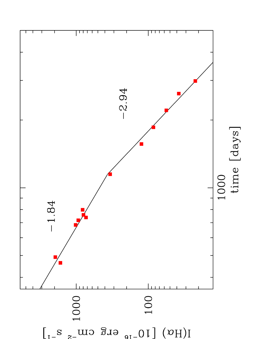
Figure 3: Evolution of the H$\alpha$ line intensity, from Aretxaga et al. (1999), during the same time range when radio observations were obtained, $\sim$300 to $\sim$3000 days after explosion. Note a likely steepening of the decline rate, $\beta$, for the H$\alpha$ intensity after $\sim 1250$ days, with $\beta_{1}=-1.84$ before the break and $\beta_{2}=-2.94$ thereafter.

Considering other wavelengths, we note that the H$\alpha$ light curve from Aretxaga et al. (1999; see their Figure 2) deviates significantly from their models after day $\sim$1000. To investigate this further, we have plotted in Figure 3 the H$\alpha$ light curve after day 300, the interval for which we have radio data. Examination of Figure 3 shows that the H$\alpha$ light curve is consistent with a slope steepening from $\beta{{}_{1}}=-1.84$ to $\beta{{}_{2}}=-2.94$ after day $\sim$1250. The H$\alpha$ emission is proportional to $\rho^{2}$, while for “typical” SNe the radio emission is proportional to $\rho^{1.4}$ (i.e., if $\beta$ is the H$\alpha$ light curve decline rate, $\beta{{}_{1}}=-1.84$ should be the same as $\sim 2/1.4\times\beta_{\rm radio}=1.42\times\beta_{\rm early}=-1.73$, where $\beta_{\rm early}=-1.22$ from Table 3). Thus, very good agreement is found between the behavior of the decline for both the early optical H$\alpha$ emission-line and early radio light curves, to within the uncertainties. Also, the change in the slope ($\Delta\beta$) at both H$\alpha$ and in the radio should be the same, because the break is due to a change in the number of clumps, not in the properties of the clumps and, therefore, should be wavelength independent: $\Delta\beta_{{\rm H}\alpha}=(-2.94)-(-1.84)=-1.10$; $\Delta\beta_{\rm radio}=(-2.73)-(-1.22)=-1.51$, which is also in fair agreement, considering the uncertainties. Thus, it appears that the steepening in the decline for the nonthermal radio light curves is consistent with the steepening of the thermal H$\alpha$ light curve.

4.1 The Mass-Loss Rate for the SN Progenitor

We can now use equations (3) and (15) to estimate from the radio absorption a mass-loss rate for the SN 1988Z progenitor star. With the assumptions for the blastwave and CSM properties discussed in §3 and the results for the best-fit parameters listed in Table 3, we obtain an estimated presupernova mass-loss rate, $\dot{M}=1.2\times 10^{-4}\ M_{\odot}$ yr^-1.

This high mass-loss rate for SN 1988Z is only appropriate for the last $\sim 10,000$ years before explosion (see §5). At earlier epochs of the progenitor’s evolution the mass-loss rate was considerably lower, as indicated by the much more steeply declining $\beta$ with unchanged $K_{3}$ and $\delta^{\prime}$ after day $\sim$1750.

5 Discussion

Figure 1, Table 3, and $\S 4$ show that the radio light curves for SN 1988Z can be described by standard RSN models (Weiler et al. 1986, 1990, 2001; Montes et al. 1997), with only one fitting parameter varying with time — the index of the time evolution of the radio emission, $\beta$. At an age of $\sim$1750 days $\beta$ clearly steepened from $\sim-1.2$ to $\sim-2.7$. This change in radio emission characteristic, $\beta$, was not accompanied by a corresponding change in the absorption characteristics, $K_{3}$ and $\delta^{\prime}$. Thus, the change in the radio light curves for SN 1988Z cannot be described as only due to a change in the average CSM density, which so effectively described the changes in radio evolution for SN 1980K (Montes et al. 1998) and SN 1979C (Montes et al. 2000).

For SN 1988Z the observations are best interpreted as a decrease in the number density of clumps in the wind-established CSM after day $\sim 1750$, but with all clumps having essentially the same average internal characteristics as at earlier times. Since the shock velocity for SN 1988Z is assumed to be $\sim 20,000$ km s^-1 and the pre-supernova wind velocity for an RSG is typically $\sim 10$ km s^-1, an interval of 1,750 days after explosion implies that this change took place in the presupernova stellar wind $\sim 9,600$ years before explosion. With an estimated mass-loss rate in the interval prior to explosion of $\sim 1.2\times 10^{-4}\ M_{\odot}$ yr^-1, it follows that during this last 10,000 years, the progenitor star shed $\sim 1.1~{}M_{\odot}$ in a massive “superwind.” The abrupt steepening of $\beta$ around day 1750 implies that the mass-loss rate was appreciably lower before that time, decreasing by about a factor of four by day 4,438. Even such a decreasing mass-loss rate, however, still accounts for an additional $\sim 0.8\ M_{\odot}$ lost in the stellar wind by our last measurement on day 4,438 ($\sim 25,000$ years before explosion, using the same wind and blastwave velocity assumptions). Since a relatively high mass-loss rate must have been maintained over a much longer time, such as the $\sim 10^{5}$ years appropriate for a massive star’s evolution, an additional several $M_{\odot}$ must have been lost earlier so that the presupernova mass loss for SN 1988Z over the entire RSG progenitor lifetime is expected to have been $>2\ M_{\odot}$, and perhaps much greater.

As discussed in $\S 1$, Chugai & Danziger (1994) studied SN 1988Z in detail and developed a model from which they concluded that the ejecta mass is small ($M_{\rm ej}<1\ M_{\odot}$), and that SN 1988Z, therefore, must have originated from a relatively low-mass star, $M_{\rm ZAMS}\sim 8$–10 ${M_{\odot}}$, in sharp contrast with the high-mass (20–40 $M_{\odot}$) progenitor proposed by Van Dyk et al. (1993a) and Stathakis & Sadler (1991). However, it should be noted that Chugai & Danziger derived a very high mass-loss rate for the SN 1988Z progenitor, $7\times 10^{-4}\ M_{\odot}$ yr^-1, yielding what they call their “wind density parameter” (our $\dot{M}/w_{\rm wind}$) of $5\times 10^{16}~{}{\rm g~{}cm^{-1}}$. We believe that our mass-loss rate derived from the direct measurement of f-f absorption in the CSM, $1.2\times 10^{-4}\ M_{\odot}$ yr^-1 (wind density parameter, $\dot{M}/w_{\rm wind}=7.3\times 10^{15}~{}{\rm g~{}cm^{-1}}$), is likely more appropriate. Since the critical factors in the modeling by Chugai & Danziger are the product of the ejecta mass and wind density parameter related to the energy of the explosion, for a given explosion energy our 6–7 times smaller wind density parameter implies, for their model, a factor of 6–7 times greater ejecta mass, $M_{\rm ej}\sim 5$–10 $M_{\odot}$, rather than their estimate of $M_{\rm ej}\leq 1\ M_{\odot}$. Even our value for the ejecta mass may still be an underestimate because, by the Chugai & Danziger model, it represents only the mass that was observed to interact with the pre-supernova wind and may not involve the entire ejecta mass. With an ejecta mass of as much as $\sim 10~{}M_{\odot}$ and a high radio luminosity, which places SN 1988Z among the brightest radio supernovae, we conclude that the stellar progenitor of SN 1988Z must have been a very massive star, perhaps as high as $\sim 20$ – 30 $M_{\odot}$, as previously suggested by Van Dyk et al. (1993a).

It is worth noting that all of the well-studied cases of ultra-bright RSNe (say, having $\geq$10 times the radio luminosity of SN 1979C at 6 cm peak), such as SNe 1988Z, 1986J, and 1998bw, provide evidence for a highly-clumped CSM with presupernova wind mass-loss rates up to $\sim 10^{-4}M_{\odot}$ yr^-1 and unusually high shock velocities $\gtrsim 20,000$  km s^-1. From optical and ultraviolet spectroscopy Fransson et al. (2002) also find for the SN IIn 1995N evidence for high shock velocities, a “superwind” phase for the progenitor characterized by a high mass-loss rate prior to explosion, and a clumpy CSM. Such high-rate mass loss, clumping of the CSM, and consequent high blastwave velocities may be the signature of particularly massive star progenitors (see also the discussion in Fransson et al. 2002). It is yet to be determined how the progenitors of SNe IIn, which must retain at least some of their hydrogen envelopes until the end of their lifetimes, and the progenitors of possibly extreme Type Ib/c SNe, such as SN 1998bw, which must have lost their entire hydrogen envelopes before explosion, are related, if at all.

6 Conclusions

The radio emission from SN 1988Z followed an evolution well described by standard models up to an age of $\sim 1750$ days ($\sim 4.8$ yrs), after which its behavior evolved into a much more rapid decline in radio emission without a corresponding change in radio absorption parameters. This is the first time we have witnessed this in any well-studied RSN, and it implies that highly radio-luminous RSNe, such as SN 1988Z and, possibly, SN 1986J, may follow a different evolutionary path in their presupernova mass-loss than that for more “normal” RSNe, such as SNe 1979C and 1980K. However, it is interesting to note that, if one assumes a blastwave velocity $\sim 2,000$ times faster than the RSG wind-established CSM ($\sim 20,000$ km s^-1 vs. $\sim 10$ km s^-1), the timescale for such a variation in SN 1988Z of $\sim 10^{4}$ yr, is similar to that seen for SNe 1979C and 1980K (see, e.g., for SN 1979C, Montes et al. 1998; for SN 1980K, Montes et al. 2000), and also for SN 1998bw (Weiler et al. 2001).

In addition, further analysis of the results from Chugai & Danziger (1994), which implied an extremely high mass-loss rate of $7\times 10^{-4}M_{\odot}$ yr^-1 and a relatively low-mass progenitor with $M_{\rm ZAMS}\sim 8$–10 $M_{\odot}$ for SN 1988Z, indicates that their estimates are probably unrealistic. Using their modeling, our lower mass-loss rate, $1.2\times 10^{-4}\ M_{\odot}$ yr^-1, implies a significantly higher ejecta mass and, therefore, a higher ZAMS mass of $\sim 20$–30 $M_{\odot}$ for the progenitor star.

We have noted that the H${\alpha}$ data from Aretxaga et al. (1999), which are also indicative of the SN shock-CSM interaction (Chevalier & Fransson 1994), also begin to deviate significantly from their model by day $\gtrsim$1250. Although a detailed comparison is beyond the scope of this paper, both the slope before the break and the magnitude of the break are roughly consistent with the radio results.

From our analysis we propose that SNe, such as SNe 1988Z, 1986J, and 1998bw (possibly the counterpart to GRB 980425), with possible very massive star progenitors ($M_{\rm ZAMS}>20\ M_{\odot}$) and associated massive winds ($\dot{M}\gtrsim 10^{-4}\ M_{\odot}$ yr^-1), have very highly-clumped, wind-established CSM and unusually high blastwave velocities ($>20,000$ km s^-1).

Table 1: Flux Density Measurements for SN 1988Z

Obs. Date	Age	VLA	$S$ (20 cm)	$S$ (6 cm)	$S$ (3.6 cm)	$S$ (2.0 cm)
(UT)	(days)	Config.	(mJy)	(mJy)	(mJy)	(mJy)
1988 Dec 1	$\equiv$ 0
1989 Dec 21	385	D	$\cdots$	$0.67\pm 0.07$	$\cdots$	$\cdots$
1990 Feb 12	438	DnA	$\cdots$	$0.77\pm 0.09$	$\cdots$	$\cdots$
1990 May 29	544	A	$\cdots$	$1.21\pm 0.09$	$\cdots$	$\cdots$
1990 Jul 12	588	BnA	$\cdots$	$1.26\pm 0.09$	$2.10\pm 0.14$	$\cdots$
1990 Sep 7	645	B	$<$0.39	$1.38\pm 0.09$	$1.72\pm 0.14$	$1.15\pm 0.23$
1990 Dec 14	743	C	$<$0.48	$1.78\pm 0.10$	$2.09\pm 0.13$	$1.43\pm 0.19$
1991 Jun 11	922	A	$0.47\pm 0.07$	$1.90\pm 0.11$	$1.68\pm 0.10$	$1.31\pm 0.25$
1991 Sep 17	1020	A	$\cdots$	$1.85\pm 0.10$	$1.48\pm 0.09$	$0.68\pm 0.16$
1992 Jan 26	1151	CnB	$1.04\pm 0.13$	$1.67\pm 0.10$	$1.50\pm 0.09$	$1.17\pm 0.18$
1992 Oct 13	1412	A	$0.91\pm 0.08$	$1.57\pm 0.09$	$1.22\pm 0.10$	$0.91\pm 0.22$
1992 Dec 19	1479	A	$1.52\pm 0.09$	$1.72\pm 0.11$	$1.04\pm 0.08$	$0.78\pm 0.19$
1993 May 4	1615	B	$1.16\pm 0.10$	$1.21\pm 0.09$	$0.98\pm 0.06$	$0.57\pm 0.15$
1993 Aug 23	1726	BnA	$1.05\pm 0.15$	$1.28\pm 0.09$	$\cdots$	$\cdots$
1993 Dec 5	1830	D	$\cdots$	$\cdots$	$0.87\pm 0.07$	$\cdots$
1994 Feb 18	1905	DnA	$1.09\pm 0.16$	$0.98\pm 0.17$	$0.86\pm 0.14$	$\cdots$
1994 May 4	1980	BnA	$1.42\pm 0.16$	$0.97\pm 0.13$	$0.52\pm 0.08$	$\cdots$
1994 Sep 30	2129	CnB	$1.06\pm 0.15$	$0.91\pm 0.05$	$0.56\pm 0.08$	$\cdots$
1995 May 19	2360	D	$\cdots$	$0.62\pm 0.05$	$0.42\pm 0.04$	$0.26\pm 0.09$
1995 Oct 3	2497	BnA	$0.78\pm 0.07$	$0.40\pm 0.04$	$0.23\pm 0.04$	$<$0.38
1996 Oct 5	2865	DnA	$0.72\pm 0.15$	$0.36\pm 0.09$	$0.32\pm 0.06$	$<$0.36
1997 Jan 23	2975	BnA	$0.68\pm 0.11$	$0.30\pm 0.08$	$\cdots$	$\cdots$
1998 Feb 10	3358	DnA	$\cdots$	$\cdots$	$<0.15$	$\cdots$
1998 Feb 13	3361	DnA	$0.35\pm 0.06$	$0.30\pm 0.05$	$\cdots$	$\cdots$
1998 Oct 19	3609	B	$0.39\pm 0.07$	$0.20\pm 0.03$	$\cdots$	$\cdots$
1999 Jun 13	3846	DnA	$0.19\pm 0.06$	$<$0.20	$\cdots$	$\cdots$
1999 Oct 1	3956	DnA	$0.22\pm 0.06$	$0.17\pm 0.04$	$\cdots$	$\cdots$
2001 Oct 19	4340	A	$0.19\pm 0.03$	$<$0.18	$<$0.18	$\cdots$
2001 Jan 25	4438	DnA	$0.17\pm 0.06$	$<$0.26	$<$0.27	$\cdots$

Table 2: Flux Density Measurements for Secondary Calibrators

Obs. Date	$S$ (20 cm)	$S$ (6 cm)	$S$ (3.6 cm)	$S$ (2.0 cm)
(UT)	(Jy)	(Jy)	(Jy)	(Jy)
J1051+213
1989 Dec 21	$\cdots$	0.921	$\cdots$	$\cdots$
1990 Feb 12	$\cdots$	0.885	$\cdots$	$\cdots$
1990 May 29	$\cdots$	0.901	$\cdots$	$\cdots$
1990 Jul 12	$\cdots$	0.907	0.894	$\cdots$
1990 Sep 7	1.092	1.002	0.942	1.123
1990 Dec 14	1.118	0.948	1.069	0.967
1991 Jun 11	0.962	0.997	1.162	1.203
1991 Sep 17	$\cdots$	1.091	1.358	1.336
J1125+261
1992 Jan 26	0.992	1.069	1.001	0.806
1992 Oct 13	0.948	1.102	0.954	0.839
1992 Dec 19	0.937	1.068	0.926	0.729
1993 May 4	0.967	1.008	0.871	0.703
1993 Aug 23	0.892	0.986	$\cdots$	$\cdots$
1993 Dec 5	$\cdots$	$\cdots$	0.887	$\cdots$
1994 Feb 18	0.910	1.049	0.934	$\cdots$
1994 May 4	0.920	1.056	0.891	$\cdots$
1994 Sep 30	0.943	1.082	0.984	$\cdots$
1995 May 19	$\cdots$	1.088	0.936	0.749
1995 Oct 3	0.880	1.098	0.966	0.781
1996 Oct 5	0.899	1.059	0.854	0.657
1997 Jan 23	0.893	1.060	$\cdots$	$\cdots$
1998 Feb 10	$\cdots$	$\cdots$	0.918	$\cdots$
1998 Feb 13	0.961	0.911	$\cdots$	$\cdots$
1998 Oct 19	0.989	0.967	$\cdots$	$\cdots$
1999 Jun 13	0.957	0.927	$\cdots$	$\cdots$
1999 Oct 1	0.937	0.988	$\cdots$	$\cdots$
2000 Oct 19	0.924	0.887	0.709	$\cdots$
2001 Jan 25	0.933	1.070	0.936	$\cdots$

Table 3: Fitting Parameters for SNe 1988Z

Parameter	SN 1988Z
	Early	Global	Late
	${\rm day}<2000$		${\rm day}>1500$
$K_{1}$	$1.2\times 10^{4}$		$9.1\times 10^{8}$
$\alpha$		$-0.72$
$\beta$	$-1.22$		$-2.73$
$K_{3}$		$3.19\times 10^{8}$
$\delta^{\prime}$		$-2.87$
$t_{0}$		$\equiv$ 1988 Dec 01
${\rm L_{6\ cm\ peak}}$ (erg s-1 Hz-1)		$2.3\times 10^{28}$
$t=(t_{\rm 6\ cm\ peak}-t_{0})$ (days)		911
$\dot{M}$ ($M_{\odot}$ yr-1)		$1.2\times 10^{-4}$

Figure 1: Radio “light curves” for SN 1988Z in MCG +03-28-022. The four wavelengths, 2 cm (14.9 GHz, open circles, solid line), 3.6 cm (8.44 GHz, crosses, dashed line), 6 cm (4.87 GHz, open squares, dot-dash line), and 20 cm (1.48 GHz, open triangles, dotted line), are shown together with their best-fit model light curves. The SN age is in days since the adopted explosion date of 1988 December 1 (Stathakis & Sadler 1991). Because the decline index $\beta$ of the radio emission steepened between, roughly, day $\sim$1500 and day $\sim$2000, an iterative fitting procedure was used (see §4), and a break in the model radio light curves can be seen near day 1750.

Figure 2: Flux density measurements of the secondary calibrators J1051+213 and J1125+261 at 2 cm (14.9 GHz, open circles), 3.6 cm (8.44 GHz, crosses), 6 cm (4.87 GHz, open squares), and 20 cm (1.48 GHz, open triangles). For clarity the data points at each frequency are offset from one another by adding 1.0 Jy to the 2 cm values, 0.5 Jy to the 3.6 cm values, and $-$0.5 Jy to the 20 cm values. The epoch at which the secondary calibrator was changed from J1051+213 to J1125+261 is marked.

References

- Aretxaga et al. (1999) Aretxaga, I., Benetti, S., Terlevich, R. J., Fabian, A. C., Cappellaro, E., Turatto, M., & della Valle, M. 1999, MNRAS, 309, 343
- Bregman & Pildis (1992) Bregman, J. N., & Pildis, R. A. 1992, ApJ, 398, L107
- Cappellaro, Turatto, & Candeo (1988) Cappellaro, E., Turatto, M., & Candeo, G. 1988, IAU Circ., 4691
- Chevalier (1982a) Chevalier, R. A. 1982a, ApJ, 259, 302
- Chevalier (1982b) Chevalier, R. A. 1982b, ApJ, 259, L85
- Chevalier & Fransson (1994) Chevalier, R. A. & Fransson, C. 1994, ApJ, 420, 268
- Chugai & Danziger (1994) Chugai, N. N. & Danziger, I. J. 1994, MNRAS, 268, 173
- Fabian & Terlevich (1996) Fabian, A. C. & Terlevich, R. 1996, MNRAS, 280, L5
- Filippenko (1989) Filippenko, A. V. 1989, IAU Circ., 4713
- Filippenko (1991a) Filippenko, A. V. 1991a, in Supernovae: The Tenth Santa Cruz Workshop in Astronomy and Astrophysics. Ed., S.E. Woosley (Springer-Verlag, New York), 467
- Filippenko (1991b) Filippenko, A. V. 1991b, in SN 1987A and Other Supernovae. Eds., I. J. Danziger and K. Kjar (ESO, Garching bei Muenchen), 343
- Filippenko, Matheson, & Barth (1994) Filippenko, A., Matheson, T., & Barth, A. 1994, AJ, 108, 222
- Fransson et al. (2002) Fransson, C., Chevalier, R. A., Filippenko, A. V., Leibundgut, B., Barth, A. J., Fesen, R. A., Kirshner, R. P., Leonard, D. C., Li, W. D., Lundqvist, P., Sollerman, J., & Van Dyk, S. D. 2002, ApJ, 572, 350
- Heathcote et al. (1988) Heathcote, S., Cowley, A., & Hartwick, D. 1988, IAU Circ., 4693
- Houck et al. (1998) Houck, J. C., Bregman, J. N., Chevalier, R. A., Tomisaka, K. 1998, ApJ, 493, 431
- Iwamoto et al. (1998) Iwamoto, K. et al. 1998, Nature, 395, 672
- Kirshner, Leibundgut, & Smith (1989) Kirshner, R., Leibundgut, B., & Smith, C. 1989, IAU Circ., 4900
- Leibundgut et al. (1991) Leibundgut, B., Kirshner, R. P., Pinto, P. A., Rupen, M. P., Smith, R. C., Gunn, J. E., & Schneider, D. P. 1991, ApJ, 372, 531
- Montes, Weiler, & Panagia (1997) Montes, M. J., Weiler, K. W., & Panagia, N. 1997, ApJ, 488, 792
- Montes et al. (1998) Montes, M. J., Van Dyk, S. D., Weiler, K. W., Sramek, R. A., & Panagia, N. 1998, ApJ, 506, 874
- Montes et al. (2000) Montes, M. J., Weiler, K. W., Van Dyk, S. D., Panagia, N., Lacey, C. K., Sramek, R. A., & Park, R. 2000, ApJ, 532, 1124
- Natta & Panagia (1984) Natta, A., & Panagia, N. 1984, ApJ, 287, 228
- Osterbrock (1974) Osterbrock, D. E. 1974, Astrophysics of Gaseous Nebulae (San Francisco; Freeman), pp. 82-87
- Pastorello et al. (2002) Pastorello, A., Turatto, M., Benetti, S., Cappellaro, E., Danziger, I. J., Mazzali, P. A., Patat, F., Filippenko, A. V., Schlegel, D. J., & Matheson T. 2002, MNRAS, 333, 27
- Pollas (1988) Pollas, C. 1988, IAU Circ., 4691
- Rupen et al. (1987) Rupen, M. P., van Gorkom, J. H., Knapp, G. R., Gunn, J. E., & Schneider, D. P. 1987, AJ, 94, 61
- Schlegel (1990) Schlegel, E. M. 1990, MNRAS, 244, 269
- Spyromilio (1994) Spyromilio, J. 1994, MNRAS, 266, 61
- Sramek, Panagia, & Weiler (1984) Sramek, R. A., Panagia, N., & Weiler, K. W. 1984, ApJ, 285, L59
- Sramek, Weiler, & Panagia (1990) Sramek, R. A., Weiler, K. W., & Panagia, N. 1990, IAU Circ., 5112
- Stathakis & Sadler (1991) Stathakis, R. A. & Sadler, E. M. 1991, MNRAS, 250, 786
- Turatto et al. (1993) Turatto, M., Cappellaro, E., Danziger, I. J., Benetti, S., Gouiffes, C., & della Valle, M. 1993, MNRAS, 262, 128
- Van Dyk et al. (1993a) Van Dyk, S., Sramek, R. A., Weiler, K., & Panagia, N. 1993a, ApJ, 419, 69
- Van Dyk et al. (1993b) Van Dyk, S. D., Sramek, R. A., Weiler, K. W., & Panagia, N. 1993b, ApJ, 409, 162
- Van Dyk et al. (1994) Van Dyk, S., Weiler, K., Sramek, R., Rupen, M., & Panagia, N. 1994, ApJ, 432, 115
- Weiler et al. (1986) Weiler, K. W., Sramek, R. A., Panagia, N., van der Hulst, J. M., & Salvati, M. 1986, ApJ, 301, 790
- Weiler, Panagia, & Sramek (1990) Weiler, K. W., Panagia, N., & Sramek, R. A. 1990, ApJ, 364, 611
- Weiler et al. (1991) Weiler, K. W., Van Dyk, S. D., Discenna, J. L., Panagia, N., & Sramek, R. A. 1991, ApJ, 380, 161
- Weiler et al. (1992a) Weiler, K. W., Van Dyk, S. D., Pringle, J., & Panagia, N. 1992a, ApJ, 399, 672
- Weiler et al. (1992b) Weiler, K. W., Van Dyk, S. D., Panagia, N., & Sramek, R. A. 1992b, ApJ, 398, 248
- Weiler, Panagia, & Montes (2001) Weiler, K. W., Panagia, N., & Montes, M. 2001, ApJ, 562, 670
- Weiler et al. (2002) Weiler, K. W., Panagia, N., Montes, M. J., & Sramek, R. A. 2002, ARA&A, 40, 387