Primordial Alchemy:
From The Big Bang To The Present Universe

Abstract

Of the light nuclides observed in the universe today, D, ³He, ⁴He, and ⁷Li are relics from its early evolution. The primordial abundances of these relics, produced via Big Bang Nucleosynthesis (BBN) during the first half hour of the evolution of the universe provide a unique window on Physics and Cosmology at redshifts $\sim 10^{10}$. Comparing the BBN-predicted abundances with those inferred from observational data tests the consistency of the standard cosmological model over ten orders of magnitude in redshift, constrains the baryon and other particle content of the universe, and probes both Physics and Cosmology beyond the current standard models. These lectures are intended to introduce students, both of theory and observation, to those aspects of the evolution of the universe relevant to the production and evolution of the light nuclides from the Big Bang to the present. The current observational data is reviewed and compared with the BBN predictions and the implications for cosmology (e.g., universal baryon density) and particle physics (e.g., relativistic energy density) are discussed. While this comparison reveals the stunning success of the standard model(s), there are currently some challenges which leave open the door for more theoretical and observational work with potential implications for astronomy, cosmology, and particle physics.

The present universe is expanding and is filled with radiation (the 2.7 K Cosmic Microwave Background – CMB) as well as “ordinary” matter (baryons), “dark” matter and, “dark energy”. Extrapolating back to the past, the early universe was hot and dense, with the overall energy density dominated by relativistic particles (“radiation dominated”). During its early evolution the universe hurtled through an all too brief epoch when it served as a primordial nuclear reactor, leading to the synthesis of the lightest nuclides: D, ³He, ⁴He, and ⁷Li. These relics from the distant past provide a unique window on the early universe, probing our standard models of cosmology and particle physics. By comparing the predicted primordial abundances with those inferred from observational data we may test the standard models and, perhaps, uncover clues to modifications or extensions beyond them.

These notes summarize the lectures delivered at the XIII Canary Islands Winter School of Astrophysics: “Cosmochemistry: The Melting Pot of Elements”. The goal of the lectures was to provide both theorists and observers with an overview of the evolution of the universe from its earliest epochs to the present, concentrating on the production, evolution, and observations of the light nuclides. Standard Big Bang Nucleosynthesis (SBBN) depends on only one free parameter, the universal density of baryons; fixing the primordial abundances fixes the baryon density at the time of BBN. But, since baryons are conserved (at least for these epochs), fixing the baryon density at a redshift $\sim 10^{10}$, fixes the present-universe baryon density. Comparing this prediction with other, independent probes of the baryon density in the present and recent universe offers the opportunity to test the consistency of our standard, hot big bang cosmological model.

Since these lectures are intended for a student audience, they begin with an overview of the physics of the early evolution of the Universe in the form of a “quick and dirty” mini-course on Cosmology (§1). The experts may wish to skip this material. With the necessary background in place, the second lecture (§2) discusses the physics of primordial nucleosynthesis and outlines the abundances predicted by the standard model. The third lecture considers the evolution of the abundances of the relic nuclides from BBN to the present and reviews the observational status of the primordial abundances (§3). As is to be expected in such a vibrant and active field of research, this latter is a moving target; the results presented here represent the status in November 2001. Armed with the predictions and the observations, the fourth lecture (§4) is devoted to the confrontation between them. As is by now well known, this confrontation is a stunning success for SBBN. However, given the precision of the predictions and of the observational data, it is inappropriate to ignore some of the potential discrepancies. In the end, these may be traceable to overly optimistic error budgets, to unidentified systematic errors in the abundance determinations, to incomplete knowledge of the evolution from the big bang to the present or, to new physics beyond the standard models. In the last lecture I present a selected overview of BBN in some non-standard models of Cosmology and Particle Physics (§5). Although I have attempted to provide a representative set of references, I am aware they are incomplete and I apologize in advance for any omissions.

1 The Early Evolution of the Universe

Observations of the present universe establish that, on sufficiently large scales, galaxies and clusters of galaxies are distributed homogeneously and they are expanding isotropically. On the assumption that this is true for the large scale universe throughout its evolution (at least back to redshifts $\sim 10^{10}$, when the universe was a few hundred milliseconds old), the relation between space-time points may be described uniquely by the Robertson – Walker Metric

$$ds^{2}=c^{2}dt^{2}-a^{2}(t)({dr^{2}\over 1-{\kappa}r^{2}}+r^{2}d\Omega^{2})\,,$$ (1.1)

where $r$ is a comoving radial coordinate and $\theta$ and $\phi$ are comoving spherical coordinates related by

$$d{\Omega}^{2}\equiv d{\theta}^{2}+sin^{2}{\theta}d{\phi}^{2}\,.$$ (1.2)

A useful alternative to the comoving radial coordinate $r$ is $\Theta$, defined by

$$d\Theta\equiv{dr\over(1-{\kappa}r^{2})^{1/2}}\,.$$ (1.3)

The 3-space curvature is described by $\kappa$, the curvature constant. For closed (bounded), or “spherical” universes, $\kappa>0$; for open (unbounded), or “hyperbolic” models, $\kappa<0$; when $\kappa=0$, the universe is spatially flat or “Euclidean”. It is the “scale factor”, $a=a(t)$, which describes how physical distances between comoving locations change with time. As the universe expands, $a$ increases while, for comoving observers, $r$, $\theta$, and $\phi$ remain fixed. The growth of the separation between comoving observers is solely due to the growth of $a$. Note that neither $a$ nor $\kappa$ is observable since a rescaling of $\kappa$ can always be compensated by a rescaling of $a$.

Photons and other massless particles travel on geodesics: $ds=0$; for them (see eq. 1.1) $d\Theta=\pm~{}cdt/a(t)$. To illustrate the significance of this result consider a photon travelling from emission at time $t_{e}$ to observation at a later time $t_{o}$. In the course of its journey through the universe the photon traverses a comoving radial distance $\Delta\Theta$, where

$$\Delta\Theta=\int^{t_{o}}_{t_{e}}~{}{cdt\over a(t)}\,.$$ (1.4)

Some special choices of $t_{e}$ or $t_{o}$ are of particular interest. For $t_{e}\rightarrow 0$, $\Delta\Theta\equiv\Theta_{\rm H}(t_{o})$ is the comoving radial distance to the “Particle Horizon” at time $t_{0}$. It is the comoving distance a photon could have travelled (in the absence of scattering or absorption) from the beginning of the expansion of the universe until the time $t_{o}$. The “Event Horizon”, $\Theta_{\rm E}(t_{e})$, corresponds to the limit $t_{o}\rightarrow\infty$ (provided that $\Theta_{\rm E}$ is finite!). It is the comoving radial distance a photon will travel for the entire future evolution of the universe, after it is emitted at time $t_{e}$.

1.1 Redshift

Light emitted from a comoving galaxy located at $\Theta_{g}$ at time $t_{e}$ will reach an observer situated at $\Theta_{o}\equiv 0$ at a later time $t_{o}$, where

$$\Theta_{g}(t_{o},t_{e})=\int^{t_{o}}_{t_{e}}~{}{cdt\over a(t)}\,.$$ (1.5)

Equation 1.5 provides the relation among $\Theta_{g}$, $t_{o}$, and $t_{e}$. For a comoving galaxy, $\Theta_{g}$ is unchanged so that differentiating eq. 1.5 leads to

$${dt_{o}\over dt_{e}}={a_{o}\over a_{e}}={\nu_{e}\over\nu_{o}}={\lambda_{o}\over\lambda_{e}}\,.$$ (1.6)

This result relates the evolution of the universe ($a_{o}/a_{e}$) as the photon travels from emission to observation, to the change in its frequency ($\nu$) or wavelength ($\lambda$). As the universe expands (or contracts!), wavelengths expand (contract) and frequencies decrease (increase). The redshift of a spectral line is defined by relating the wavelength at emission (the “lab” or “rest-frame” wavelength $\lambda_{e}$) to the wavelength observed at a later time $t_{o}$, $\lambda_{o}$.

$$z\equiv{\lambda_{o}-\lambda_{e}\over\lambda_{e}}~{}\Longrightarrow~{}1+z={a_{o}\over a_{e}}={\nu_{e}\over\nu_{o}}\,.$$ (1.7)

Since the energies of photons are directly proportional to their frequencies, as the universe expands photon energies redshift to smaller values: E${}_{\gamma}=h\nu\Longrightarrow~{}$E${}_{\gamma}\propto(1+z)^{-1}$. For all particles, massless or not, de Broglie told us that wavelength and momentum are inversely related, so that: p  $\propto~{}\lambda^{-1}\Longrightarrow~{}$p$~{}\propto~{}(1+z)^{-1}$. All momenta redshift; for non-relativistic particles (e.g., galaxies) this implies that their “peculiar” velocities redshift: v = p/M $\propto(1+z)^{-1}$.

1.2 Dynamics

Everything discussed so far has been “geometrical”, relying only on the form of the Robertson-Walker metric. To make further progress in understanding the evolution of the universe, it is necessary to determine the time dependence of the scale factor $a(t)$. Although the scale factor is not an observable, the expansion rate, the Hubble parameter, $H=H(t)$, is.

$$H(t)\equiv{1\over a}({da\over dt})\,.$$ (1.8)

The present value of the Hubble parameter, often referred to as the Hubble “constant”, is $H_{0}\equiv H(t_{0})\equiv 100~{}h$ km s^-1Mpc^-1 (throughout, unless explicitly stated otherwise, the subscript “0” indicates the present time). The inverse of the Hubble parameter provides an expansion timescale, $H_{0}^{-1}=9.78~{}h^{-1}$ Gyr. For the HST Key Project (Freedman et al. 2001) value of $H_{0}=72$ km s^-1Mpc^-1 ($h=0.72$), $H_{0}^{-1}=13.6$ Gyr.

The time-evolution of $H$ describes the evolution of the universe. Employing the Robertson-Walker metric in the Einstein equations of General Relativity (relating matter/energy content to geometry) leads to the Friedmann equation

$$H^{2}={8\pi\over 3}G\rho-{\kappa c^{2}\over a^{2}}\,.$$ (1.9)

It is convenient to introduce a dimensionless density parameter, $\Omega$, defined by

$$\Omega\equiv{8\pi G\rho\over 3H^{2}}\,.$$ (1.10)

We may rearrange eq. 1.9 to highlight the relation between matter content and geometry

$$\kappa c^{2}=(aH)^{2}(\Omega-1)\,.$$ (1.11)

Although, in general, $a$, $H$, and $\Omega$ are all time-dependent, eq. 1.11 reveals that if ever $\Omega<1$, then it will always be $<1$ and in this case the universe is open ($\kappa<0$). Similarly, if ever $\Omega>1$, then it will always be $>1$ and in this case the universe is closed ($\kappa>0$). For the special case of $\Omega=1$, where the density is equal to the “critical density” $\rho_{\rm crit}\equiv 3H^{2}/8\pi G$, $\Omega$ is always unity and the universe is flat (Euclidean 3-space sections; $\kappa=0$).

The Friedmann equation (eq. 1.9) relates the time-dependence of the scale factor to that of the density. The Einstein equations yield a second relation among these which may be thought of as the surrogate for energy conservation in an expanding universe.

$${d\rho\over\rho}+3(1+{p\over\rho}){da\over a}=0\,.$$ (1.12)

For “matter” (non-relativistic matter; often called “dust”), $p\ll\rho$, so that $\rho/\rho_{0}=(a_{0}/a)^{3}$. In contrast, for “radiation” (relativistic particles) $p=\rho/3$, so that $\rho/\rho_{0}=(a_{0}/a)^{4}$. Another interesting case is that of the energy density and pressure associated with the vacuum (the quantum mechanical vacuum is not empty!). In this case $p=-\rho$, so that $\rho=\rho_{0}$. This provides a term in the Friedmann equation entirely equivalent to Einstein’s “cosmological constant” $\Lambda$. More generally, for $p=w\rho$, $\rho/\rho_{0}=(a_{0}/a)^{3(1+w)}$.

Allowing for these three contributions to the total energy density, eq. 1.9 may be rewritten in a convenient dimensionless form

$$({H\over H_{0}})^{2}=\Omega_{\rm M}({a_{0}\over a})^{3}+\Omega_{\rm R}({a_{0}\over a})^{4}+\Omega_{\rm\Lambda}+(1-\Omega)({a_{0}\over a})^{2}\,,$$ (1.13)

where $\Omega\equiv\Omega_{\rm M}+\Omega_{\rm R}+\Omega_{\rm\Lambda}$.

Since our universe is expanding, for the early universe ($t\ll t_{0}$) $a\ll a_{0}$, so that it is the “radiation” term in eq. 1.13 which dominates; the early universe is radiation-dominated (RD). In this case $a\propto t^{1/2}$ and $\rho\propto t^{-2}$, so that the age of the universe or, equivalently, its expansion rate is fixed by the radiation density. For thermal radiation, the energy density is only a function of the temperature ($\rho_{\rm R}\propto T^{4}$).

1.2.1 Counting Relativistic Degrees of Freedom

It is convenient to write the total (radiation) energy density in terms of that in the CMB photons

$$\rho_{\rm R}\equiv({g_{eff}\over 2})\rho_{\gamma}\,,$$ (1.14)

where $g_{eff}$ counts the “effective” relativistic degrees of freedom. Once $g_{eff}$ is known or specified, the time – temperature relation is determined. If the temperature is measured in energy units ($kT$), then

$$t({\rm sec})=({2.4\over g_{eff}^{1/2}})T^{-2}_{\rm MeV}\,.$$ (1.15)

If more relativistic particles are present, $g_{eff}$ increases and the universe would expand faster so that, at fixed $T$, the universe would be younger. Since the synthesis of the elements in the expanding universe involves a competition between reaction rates and the universal expansion rate, $g_{eff}$ will play a key role in determining the BBN-predicted primordial abundances.

• Photons

  Photons are vector bosons. Since they are massless, they have only two degress of freedom: $g_{eff}=2$. At temperature $T$ their number density is $n_{\gamma}=411(T/2.726K)^{3}~{}$cm${}^{-3}=10^{31.5}T^{3}_{\rm MeV}~{}$cm^-3, while their contribution to the total radiation energy density is $\rho_{\gamma}=0.261(T/2.726K)^{4}$ eV cm^-3. Taking the ratio of the energy density to the number density leads to the average energy per photon $\langle{\rm E}_{\gamma}\rangle=\rho_{\gamma}/n_{\gamma}=2.70~{}kT$. All other relativistic bosons may be simply related to photons by

  $${n_{\rm B}\over n_{\gamma}}={g_{\rm B}\over 2}({T_{\rm B}\over T_{\gamma}})^{3}\,,~{}~{}~{}~{}~{}~{}{\rho_{\rm B}\over\rho_{\gamma}}={g_{\rm B}\over 2}({T_{\rm B}\over T_{\gamma}})^{4}\,,~{}~{}~{}~{}~{}~{}\langle{\rm E}_{\rm B}\rangle=2.70~{}kT_{\rm B}\,.$$ (1.16)

  The $g_{\rm B}$ are the boson degrees of freedom (1 for a scalar, 2 for a vector, etc.). In general, some bosons may have decoupled from the radiation background and, therefore, they will not necessarily have the same temperature as do the photons ($T_{\rm B}\neq T_{\gamma}$).

• Relativistic Fermions

  Accounting for the difference between the Fermi-Dirac and Bose-Einstein distributions, relativistic fermions may also be related to photons

  $${n_{\rm F}\over n_{\gamma}}={3\over 4}{g_{\rm F}\over 2}({T_{\rm F}\over T_{\gamma}})^{3}\,,~{}~{}~{}~{}~{}~{}{\rho_{\rm F}\over\rho_{\gamma}}={7\over 8}{g_{\rm F}\over 2}({T_{\rm F}\over T_{\gamma}})^{4}\,,~{}~{}~{}~{}~{}~{}\langle{\rm E}_{\rm F}\rangle=3.15~{}kT_{\rm F}\,.$$ (1.17)

  $g_{\rm F}$ counts the fermion degrees of freedom. For example, for electrons (spin up, spin down, electron, positron) $g_{\rm F}=4$, while for neutrinos (lefthanded neutrino, righthanded antineutrino) $g_{\rm F}=2$.

Accounting for all of the particles present at a given epoch in the early (RD) evolution of the universe,

$$g_{eff}~{}=~{}\Sigma_{\rm B}~{}g_{\rm B}({T_{\rm B}\over T_{\gamma}})^{4}~{}+~{}{7\over 8}~{}\Sigma_{\rm F}~{}g_{\rm F}({T_{\rm F}\over T_{\gamma}})^{4}\,.$$ (1.18)

For example, for the standard model particles at temperatures $T_{\gamma}\approx$ few MeV there are photons, electron-positron pairs, and three “flavors” of lefthanded neutrinos (along with their righthanded antiparticles). At this stage all these particles are in equilibrium so that $T_{\gamma}=T_{e}=T_{\nu}$ where $\nu\equiv\nu_{e}$, $\nu_{\mu}$, $\nu_{\tau}$. As a result

$$g_{eff}=2+{7\over 8}(4+3\times 2)={43\over 4}\,,$$ (1.19)

leading to a time – temperature relation: $t=0.74~{}T^{-2}_{\rm Mev}$ sec.

As the universe expands and cools below the electron rest mass energy, the $e^{\pm}\;$pairs annihilate, heating the CMB photons, but not the neutrinos which have already decoupled. The decoupled neutrinos continue to cool by the expansion of the universe ($T_{\nu}\propto a^{-1}$), as do the photons which now have a higher temperature $T_{\gamma}=(11/4)^{1/3}T_{\nu}$ ($n_{\gamma}/n_{\nu}=11/3$). During these epochs

$$g_{eff}=2+{7\over 8}\times 3\times 2({4\over 11})^{4/3}=3.36\,,$$ (1.20)

leading to a modified time – temperature relation: $t=1.3~{}T^{-2}_{\rm Mev}$ sec.

1.2.2 “Extra” Relativistic Energy

Suppose there is some new physics beyond the standard model of particle physics which leads to “extra” relativistic energy so that $\rho_{\rm R}\rightarrow\rho_{\rm R}^{\prime}\equiv\rho_{\rm R}+\rho_{X}$; hereafter, for convenience of notation, the subscript R will be dropped. It is useful, and conventional, to account for this extra energy in terms of the equivalent number of extra neutrinos: $\Delta N_{\nu}\equiv\rho_{X}/\rho_{\nu}$ (Steigman, Schramm, & Gunn 1977 (SSG); see also Hoyle & Tayler 1964, Peebles 1966, Shvartsman 1969). In the presence of this extra energy, prior to $e^{\pm}\;$annihilation

$${\rho^{\prime}\over\rho_{\gamma}}={43\over 8}~{}(1+{7\Delta N_{\nu}\over 43})=5.375~{}(1+0.1628~{}\Delta N_{\nu})\,.$$ (1.21)

In this case the early universe would expand faster than in the standard model. The pre-$e^{\pm}\;$annihilation speedup in the expansion rate is

$$S_{pre}\equiv{t\over t^{\prime}}=({\rho^{\prime}\over\rho})^{1/2}=(1+0.1628~{}\Delta N_{\nu})^{1/2}\,.$$ (1.22)

After $e^{\pm}\;$annihilation there are similar, but quantitatively different changes

$${\rho^{\prime}\over\rho_{\gamma}}=1.681~{}(1+0.1351~{}\Delta N_{\nu})\,,~{}~{}~{}~{}~{}~{}~{}~{}S_{post}=(1+0.1351~{}\Delta N_{\nu})^{1/2}\,.$$ (1.23)

Armed with an understanding of the evolution of the early universe and its particle content, we may now proceed to the main subject of these lectures, primordial nucleosynthesis.

2 Big Bang Nucleosynthesis and the Primordial Abundances

Since the early universe is hot and dense, interactions among the various particles present are rapid and equilibrium among them is established quickly. But, as the universe expands and cools, there are departures from equilibrium; these are at the core of the most interesting themes of our story.

2.1 An Early Universe Chronology

At temperatures above a few MeV, when the universe is tens of milliseconds old, interactions among photons, neutrinos, electrons, and positrons establish and maintain equilibrium ($T_{\gamma}=T_{\nu}=T_{e}$). When the temperature drops below a few MeV the weakly interacting neutrinos decouple, continuing to cool and dilute along with the expansion of the universe ($T_{\nu}\propto a^{-1}$, $n_{\nu}\propto T_{\nu}^{3}$, and $\rho_{\nu}\propto T_{\nu}^{4}$).

2.1.1 Neutron – Proton Interconversion

Up to now we haven’t considered the baryon (nucleon) content of the universe. At these early times there are neutrons and protons present whose relative abundance is determined by the usual weak interactions.

$$p+e^{-}~{}\Longleftrightarrow~{}n+\nu_{e}\,,~{}~{}~{}~{}n+e^{+}~{}\Longleftrightarrow~{}p+\bar{\nu}_{e}\,,~{}~{}~{}~{}n~{}\Longleftrightarrow~{}p+e^{-}+\bar{\nu}_{e}\,.$$ (2.24)

As time goes by and the universe cools, the lighter protons are favored over the heavier neutrons and the neutron-to-proton ratio decreases, initially as $n/p\propto$ exp$(-\Delta m/T)$, where $\Delta m=1.29$ MeV is the neutron-proton mass difference. As the temperature drops below roughly 0.8 MeV, when the universe is roughly one second old, the rate of the two-body collisions in eq. 2.24 becomes slow compared to the universal expansion rate and deviations from equilibrium occur. This is often referred to as “freeze-out”, but it should be noted that the $n/p$ ratio continues to decrease as the universe expands, albeit at a slower rate than if the ratio tracked the exponential. Later, when the universe is several hundred seconds old, a time comparable to the neutron lifetime ($\tau_{n}=885.7\pm 0.8$ sec.), the $n/p$ ratio resumes falling exponentially: $n/p\propto$ exp$(-t/\tau_{n})$. Notice that the $n/p$ ratio at BBN depends on the competition between the weak interaction rates and the early universe expansion rate so that any deviations from the standard model (e.g., $\rho\rightarrow\rho+\rho_{X}$) will change the relative numbers of neutrons and protons available for building more complex nuclides.

2.1.2 Building The Elements

At the same time that neutrons and protons are interconverting, they are also colliding among themselves to create deuterons: $n+p\Longleftrightarrow D+\gamma$. However, at early times when the density and average energy of the CMB photons is very high, the newly-formed deuterons find themselves bathed in a background of high energy gamma rays capable of photodissociating them. As we shall soon see, there are more than a billion photons for every nucleon in the universe so that before a neutron or a proton can be added to D to begin building the heavier nuclides, the D is photodissociated. This bottleneck to BBN beginning in earnest persists until the temperature drops sufficiently so that there are too few photons energetic enough to photodissociate the deuterons before they can capture nucleons to launch BBN. This occurs after $e^{\pm}\;$annihilation, when the universe is a few minutes old and the temperature has dropped below 80 keV (0.08 MeV).

Once BBN begins in earnest, neutrons and protons quickly combine to form D, ³H, ³He, and ⁴He. Here, there is another, different kind of bottleneck. There is a gap at mass-5; there is no stable mass-5 nuclide. To jump the gap requires ⁴He reactions with D or ³H or ³He, all of which are positively charged. The coulomb repulsion among these colliding nuclei suppresses the reaction rate ensuring that virtually all of the neutrons available for BBN are incorporated in ⁴He (the most tightly bound of the light nuclides), and also that the abundances of the heavier nuclides are severely depressed below that of ⁴He (and even of D and ³He). Recall that ³H is unstable and will decay to ³He. The few reactions which manage to bridge the mass-5 gap mainly lead to mass-7 (⁷Li, or ⁷Be which later, when the universe has cooled further, will capture an electron and decay to ⁷Li); the abundance of ⁶Li is below that of the more tightly bound ⁷Li by one to two orders of magnitude. There is another gap at mass-8. This absence of any stable mass-8 nuclides ensures there will be no astrophysically interesting production of heavier nuclides.

The primordial nuclear reactor is short-lived, quickly encountering an energy crisis. Because of the falling temperatures and the coulomb barriers, nuclear reactions cease rather abruptly when the temperature drops below roughly 30 keV, when the universe is about 20 minutes old. As a result there is “nuclear freeze-out” since no already existing nuclides are destroyed (except for those that are unstable and decay) and no new nuclides are created. In $\sim 1000$ seconds BBN has run its course.

2.2 The SBBN-Predicted Abundances

The primordial abundances of D, ³He, and ⁷Li(⁷Be) are rate limited, depending sensitively on the competition between the nuclear reactions rates and the universal expansion rate. As a result, these nuclides are potential baryometers since their abundances are sensitive to the universal density of nucleons. As the universe expands, the nucleon density decreases so it is useful to compare the nucleon density to that of the CMB photons $\eta\equiv n_{\rm N}/n_{\gamma}$. Since this ratio will turn out to be very small, it is convenient to introduce

$$\eta_{10}\equiv 10^{10}(n_{\rm N}/n_{\gamma})=274\Omega_{\rm B}h^{2}\,.$$ (2.25)

As the universe evolves (post-$e^{\pm}\;$annihilation) this ratio is accurately preserved so that $\eta_{\rm BBN}=\eta_{0}$. Testing this relation over ten orders of magnitude in redshift, over a range of some ten billion years, can provide a confirmation of or a challenge to the standard model.

In contrast to the other light nuclides, the primordial abundance of ⁴He (mass fraction Y) is relatively insensitive to the baryon density, but since virtually all neutrons available at BBN are incorporated in ⁴He, it does depend on the competition between the weak interaction rate (largely fixed by the accurately measured neutron lifetime) and the universal expansion rate (which depends on $g_{eff}$). The higher the nucleon density, the earlier can the D-bottleneck be breached. At early times there are more neutrons and, therefore, more ⁴He will be synthesized. This latter effect is responsible for the very slow (logarithmic) increase in Y with $\eta$. Given the standard model relation between time and temperature and the nuclear and weak cross sections and decay rates measured in the laboratory, the evolution of the light nuclide abundances may be calculated and the frozen-out relic abundances predicted as a function of the one free parameter, the nucleon density or $\eta$. These are shown in Figure 1.

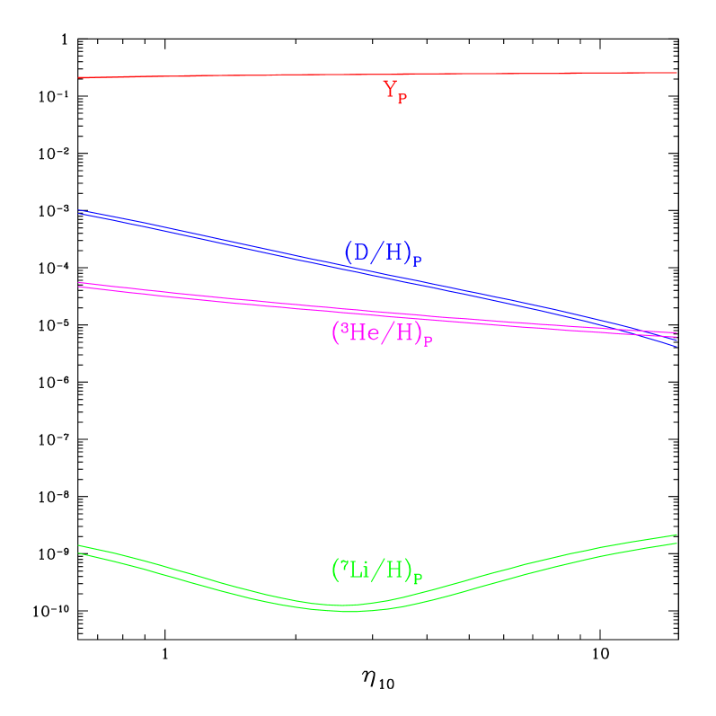
Figure 1: The SBBN-predicted primordial abundances of D, ³He, ⁷Li (by number with respect to hydrogen), and the ⁴He mass fraction Y as a function of the nucleon abundance $\eta_{10}$. The widths of the bands reflect the theoretical uncertainties.

Not shown on Figure 1 are the relic abundances of ⁶Li, ⁹Be, ¹⁰B, and ¹¹B, all of which, over the same range in $\eta$, lie offscale, in the range $10^{-20}-10^{-13}$.

The reader may notice the abundances appear in Figure 1 as bands. These represent the theoretical uncertainties in the predicted abundances. For D/H and ³He/H they are at the $\sim 8\%$ level, while they are much larger, $\sim 12\%$, for ⁷Li. The reader may not notice that a band is also shown for ⁴He, since the uncertainty in Y is only at the $\sim 0.2\%$ level ($\sigma_{\rm Y}\approx 0.0005$). The results shown here are from the BBN code developed and refined over the years by my colleagues at The Ohio State University. They are in excellent agreement with the published results of the Chicago group (Burles, Nollett & Turner 2001) who, in a reanalysis of the relevant published cross sections have reduced the theoretical errors by roughly a factor of three for D and ³He and a factor of two for ⁷Li. The uncertainty in Y is largely due to the (very small) uncertainty in the neutron lifetime.

The trends shown in Figure 1 are easy to understand based on our previous discussion. D and ³He are burned to ⁴He. The higher the nucleon density, the faster this occurs, leaving behind fewer nuclei of D or ³He. The very slight increase of Y with $\eta$ is largely due to BBN starting earlier, at higher nucleon density (more complete burning of D, ³H, and ³He to ⁴He) and neutron-to-proton ratio (more neutrons, more ⁴He). The behavior of ⁷Li is more interesting. At relatively low values of $\eta~{}\lower 2.58334pt\vbox{\hbox{$\buildrel\textstyle<\over{\sim}\ $}}3$, mass-7 is largely synthesized as ⁷Li (by ³H($\alpha$,$\gamma$)⁷Li reactions) which is easily destroyed in collisons with protons. So, as $\eta$ increases at low values, ⁷Li/H decreases. However, at relatively high values of $\eta~{}\lower 2.58334pt\vbox{\hbox{$\buildrel\textstyle>\over{\sim}\ $}}3$, mass-7 is largely synthesized as ⁷Be (via ³He($\alpha$,$\gamma$)⁷Be reactions) which is more tightly bound than ⁷Li and, therefore, harder to destroy. As $\eta$ increases at high values, the abundance of ⁷Be increases. Later in the evolution of the universe, when it is cooler and neutral atoms begin to form, ⁷Be will capture an electron and $\beta$-decay to ⁷Li.

2.3 Variations On A Theme: Non-Standard BBN

Before moving on, let’s take a diversion to which we’ll return again in §5. Suppose the standard model is modified through the addition of extra relativistic particles ($\Delta N_{\nu}\;$$>0$; SSG). Equivalently (ignoring some small differences), it could be that the gravitational constant in the early universe differs from its present value ($G\rightarrow G^{\prime}\neq G$). Depending on whether $G^{\prime}>G$ or $G^{\prime}<G$, the early universe expansion rate can be speeded up or slowed down compared to the standard rate. For concreteness, let’s assume that $S>1$. Now, there will be less time to destroy D and ³He, so their relic abundances will increase relative to the SBBN prediction. There is less time for neutrons to transform to protons. With more neutrons available, more ⁴He will be synthesized. The changes in ⁷Li are more complex. At low $\eta$ there is less time to destroy ⁷Li, so the relic ⁷Li abundance increases. At high $\eta$ there is less time to produce ⁷Be, so the relic ⁷Li (mass-7) abundance decreases.

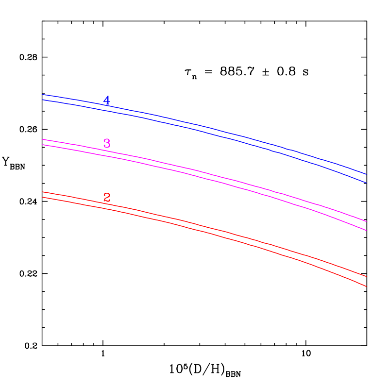
Figure 2: The BBN-predicted primordial ⁴He mass fraction Y as a function of the BBN-predicted primordial Deuterium abundance (by number relative to Hydrogen) for three choices of N_ν. The width of the bands represents the theoretical uncertainty, largely due to that of the neutron lifetime $\tau_{n}$.

Since the ⁴He mass fraction is relatively insensitive to the baryon density, it provides an excellent probe of any changes in the expansion rate. The faster the universe expands, the less time for neutrons to convert to protons, the more ⁴He will be synthesized. The increase in Y for “modest” changes in $S$ is roughly $\Delta$Y $\approx 0.16(S-1)\approx 0.013\Delta N_{\nu}$. In Figure 2 are shown the BBN-predicted Y versus the BBN-predicted Deuterium abundance (relative to Hydrogen) for three choices of N_ν (N${}_{\nu}\equiv 3+\Delta N_{\nu}$).

3 Observational Status of the Relic Abundances

Armed with the SBBN-predicted primordial abundances, as well as with those in a variation on the standard model, we now turn to the observational data. The four light nuclides of interest, D, ³He, ⁴He, and ⁷Li follow different evolutionary paths in the post-BBN universe. In addition, the observations leading to their abundance determinations are different for all four. Neutral D is observed in absorption in the UV; singly-ionized ³He is observed in emission in galactic H $\scriptstyle{\rm II}$ regions; both singly- and doubly-ionized ⁴He are observed in emission via their recombinations in extragalactic H $\scriptstyle{\rm II}$ regions; ⁷Li is observed in absorption in the atmospheres of very metal-poor halo stars. The different histories and observational strategies provides some insurance that systematic errors affecting the inferred primordial abundances of any one of the light nuclides will not influence the inferred abundances of the others.

3.1 Deuterium

The post-BBN evolution of D is simple. As gas is incorporated into stars the very loosely bound deuteron is burned to ³He (and beyond). Any D which passes through a star is destroyed. Furthermore, there are no astrophysical sites where D can be produced in an abundance anywhere near that which is observed (Epstein, Lattimer, & Schramm 1976). As a result, as the universe evolves and gas is cycled through generations of stars, Deuterium is only destroyed. Therefore, observations of the deuterium abundance anywhere, anytime, provide lower bounds on its primordial abundance. Furthermore, if D can be observed in “young” systems, in the sense of very little stellar processing, the observed abundance should be very close to the primordial value. Thus, while there are extensive data on deuterium in the solar system and the local interstellar medium (ISM) of the Galaxy, it is the handful of observations of deuterium absorption in high-redshift (hi-$z$), low-metallicity (low-Z), QSO absorption-line systems (QSOALS) which are, potentially the most valuable. In Figure 3 the extant data (circa November 2001) are shown for D/H as a function of redshift from the work of Burles & Tytler (1998a,b), O’Meara et al. (2001), D’Odorico et al. (2001), and Pettini & Bowen (2001). Also shown for comparison are the local ISM D/H (Linsky & Wood 2000) and that for the presolar nebula as inferred from solar system data (Geiss & Gloeckler 1998, Gloeckler & Geiss 2000).

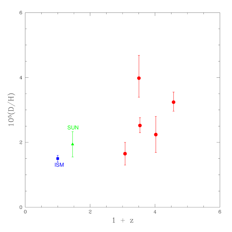
Figure 3: The deuterium abundance, D/H, versus redshift, z, from observations of QSOALS (filled circles). Also shown for comparison are the D-abundances for the local ISM (filled square) and the solar system (“Sun”; filled triangle).

On the basis of our discussion of the post-BBN evolution of D/H, it would be expected that there should be a “Deuterium Plateau” at high redshift. If, indeed, one is present, the dispersion in the limited set of current data hide it. Alternatively, to explore the possibility that the D-abundances may be correlated with the metallicity of the QSOALS, we may plot the observed D/H versus the metallicity, as measured by [Si/H], for these absorbers. This is shown in Figure 4 where there is some evidence for an (unexpected!) increase in D/H with decreasing [Si/H]; once again, the dispersion in D/H hides any plateau.

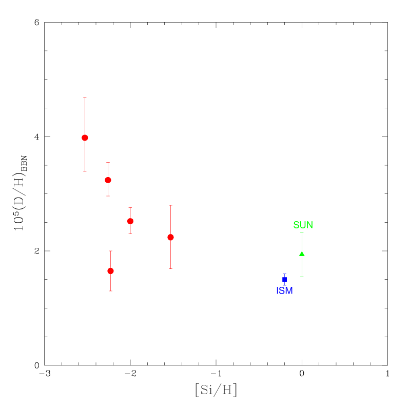
Figure 4: The deuterium abundance, D/H, versus metallicity ([Si/H]) for the same QSOALS as in Figure 3 (filled circles). Also shown for comparison are the D-abundances for the local ISM (filled square) and the solar system (“Sun”; filled triangle).

Aside from observational errors, there are several sources of systematic error which may account for the observed dispersion. For example, the Ly$\alpha$ absorption of H $\scriptstyle{\rm I}$ in these systems is saturated, potentially hiding complex velocity structure. Usually, but not always, this velocity structure can be revealed in the higher lines of the Lyman series and, expecially, in the narrower metal-absorption lines. Recall, also, that the lines in the Lyman series of D $\scriptstyle{\rm I}$ are identical to those of H $\scriptstyle{\rm I}$, only shifted by $\approx$ 81 km/s. Given the highly saturated H $\scriptstyle{\rm I}$ Ly$\alpha$, it may be difficult to identify which, and how much, of the H $\scriptstyle{\rm I}$ corresponds to an absorption feature identified as D $\scriptstyle{\rm I}$ Ly$\alpha$. Furthermore, are such features really D $\scriptstyle{\rm I}$ or, an interloping, low column density H $\scriptstyle{\rm I}$-absorber? After all, there are many more low-, rather than high-column density H $\scriptstyle{\rm I}$ systems. Statistically, the highest column density absorbers may be more immune to these systematic errors. Therefore, in Figure 5 are shown the very same D/H data, now plotted against the neutral hydrogen column density. The three highest column density absorbers (Damped Ly$\alpha$ Absorbers: DLAs) fail to reveal the D-plateau, although it may be the case that some of the D associated with the two lower column density systems may be attributable to an interloper, which would reduce the D/H inferred for them.

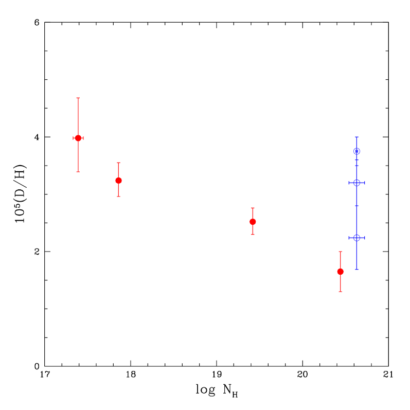
Figure 5: The same QSOALS D/H data as in Figures 3 & 4 versus the H $\scriptstyle{\rm I}$ column density (log scale). The open circle symbols are for the original (D’Odorico et al. 2001) and the revised (Levshakov et al. 2002) D/H values for Q0347-3819.

Actually, the situation is even more confused. The highest column density absorber, from D’Odorico et al. (2001), was reobserved by Levshakov et al. (2002) and revealed to have a more complex velocity structure. As a result, the D/H has been revised from $2.24\times 10^{-5}$ to $3.2\times 10^{-5}$ to $3.75\times 10^{-5}$. To this theorist, at least, this evolution suggests that the complex velocity structure in this absorber renders it suspect for determining primordial D/H. The sharp-eyed reader may notice that if this D/H determination if removed from Figure 5, there is a hint of an anticorrelation between D/H and N_H among the remaining data points, suggesting that interlopers may be contributing to (but not necessarily dominating) the inferred D $\scriptstyle{\rm I}$ column density.

However, the next highest column density H $\scriptstyle{\rm I}$-absorber (Pettini & Bowen 2001), has the lowest D/H ratio, at a value indistinguishable from the ISM and solar system abundances. Why such a high-$z$, low-Z system should have destroyed so much of its primordial D so early in the evolution of the universe, apparently without producing very many heavy elements, is a mystery. If, for no really justifiable reason, this system is arbitrarily set aside, only the three “UCSD” systems of Burles & Tytler (1998a,b) and O’Meara et al. (2001) remain. The weighted mean for these three absorbers is D/H $=3.0\times 10^{-5}$. O’Meara et al. note the larger than expected dispersion, even for this subset of D-abundances, and they suggest increasing the formal error in the mean, leading to: (D/H)${}_{\rm P}=3.0\pm 0.4\times 10^{-5}$. I will be even more cautious; when the SBBN predictions are compared with the primordial abundances inferred from the data, I will adopt: (D/H)${}_{\rm P}=3.0^{+1.0}_{-0.5}\times 10^{-5}$. Since the primordial D abundance is sensitive to the baryon abundance (D/H $\propto\eta^{-1.6}$), even these perhaps overly generous errors will still result in SBBN-derived baryon abundances which are accurate to 10 – 20%.

3.2 Helium-3

The post-BBN evolution of ³He is much more complex than that of D. Indeed, when D is incorporated into a star it is rapidly burned to ³He, increasing the ³He abundance. The more tightly bound ³He, with a larger coulomb barrier, is more robust than D to nuclear burning. Nonetheless, in the hotter interiors of most stars ³He is burned to ⁴He and beyond. However, in the cooler, outer layers of most stars, and throughout most of the volume of the cooler, lower mass stars, ³He is preserved (Iben 1967, Rood, Steigman, & Tinsley 1976; Iben & Truran 1978, Dearborn, Schramm, & Steigman 1986; Dearborn, Steigman, & Tosi 1996). As a result, prestellar ³He is enhanced by the burning of prestellar D, and some, but not all, of this ³He survives further stellar processing. However, there’s more to the story. As stars burn hydrogen to helium and beyond, some of their newly synthesized ³He will avoid further processing so that the cooler, lower mass stars should be significant post-BBN sources of ³He.

Aside from studies of meteorites and in samples of the lunar soil (Reeves et al. 1973, Geiss & Gloeckler 1998, Gloeckler & Geiss 2000), ³He is only observed via its hyperfine line (of singly-ionized ³He) in interstellar H $\scriptstyle{\rm II}$ regions in the Galaxy. It is, therefore, unavoidable that models of stellar yields and Galactic chemical evolution are required in order to go from here and now (ISM) to there and then (BBN). It has been clear since the early work of Rood, Steigman and Tinsley (1976) that according to such models, ³He should have increased from the big bang and, indeed, since the formation of the solar system (see, e.g., Dearborn, Steigman & Tosi 1996 and further references therein). For an element whose abundance increases with stellar processing, there should also be a clear gradient in abundance with galactocentric distance. Neither of these expectations is borne out by the data (Rood, Bania & Wilson 1992; Balser et al. 1994, 1997, 1999; Bania, Rood & Balser 2002) which shows no increase from the time of the formation of the solar system, nor any gradient within the Galaxy. The most likely explanation is that before the low mass stars can return their newly processed ³He to the interstellar medium, it is mixed to the hotter interior and destroyed (Charbonnel 1995, Hogan 1995). Whatever the explanation, the data suggest that for ³He there is a delicate balance between production and destruction. As a result, the model-dependent uncertainties in extrapolating from the present data to the primordial abundances are large, limiting the value of ³He as a baryometer. For this reason I will not dwell further on ³He in these lectures; for further discussion and references, the interested reader is referred to the excellent review by Tosi (2000).

3.3 Helium-4

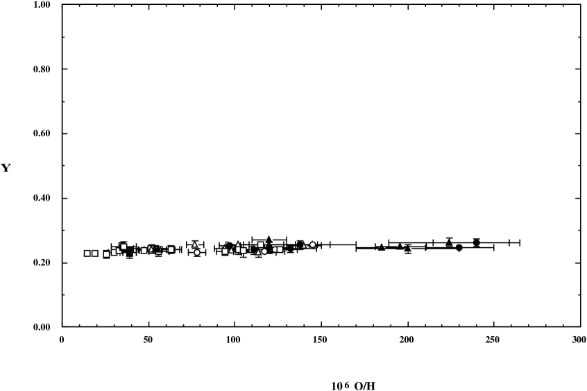
Figure 6: The ⁴He mass fraction, Y, inferred from observations of low-metallicity, extragalactic H $\scriptstyle{\rm II}$ regions versus the oxygen abundance in those regions.

Helium-4 is the second most abundant nuclide in the universe, after hydrogen. In the post-BBN epochs the net effect of gas cycling though generations of stars is to burn hydrogen to helium, increasing the ⁴He abundance. As with deuterium, a ⁴He “plateau” is expected at low metallicity. Although ⁴He is observed in the Sun and in Galactic H $\scriptstyle{\rm II}$ regions, the most relevant data for inferring its primordial abundance (the plateau value) is from observations of the helium and hydrogen recombination lines in low-metallicity, extragalactic H $\scriptstyle{\rm II}$ regions. The present inventory of such observations is approaching of order 100. It is, therefore, not surprising that even with modest observational errors for any individual H $\scriptstyle{\rm II}$ region, the statistical uncertainty in the inferred primordial abundance may be quite small. Especially in this situation, care must be taken with hitherto ignored or unaccounted for corrections and systematic errors.

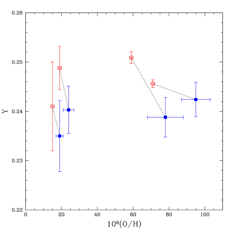
Figure 7: The Peimbert, Peimbert, & Luridiana (2002) reanalysis of the Helium-4 abundance data for 4 of the IT H $\scriptstyle{\rm II}$ regions. The open circles are the IT abundances, while the filled circles are from PPL.

In Figure 6 is shown a compilation of the data used by Olive & Steigman (1995) and Olive, Skillman, & Steigman (1997), along with the independent data from Izotov, Thuan, & Lipovetsky (1997) and Izotov & Thuan (1998). To track the evolution of the ⁴He mass fraction, Y is plotted versus the H $\scriptstyle{\rm II}$ region oxygen abundance. These H $\scriptstyle{\rm II}$ regions are all metal-poor, ranging from $\sim 1/2$ down to $\sim 1/30$ of solar (for a solar oxygen abundance of O/H $=5\times 10^{-4}$; Allende-Prieto, Lambert, & Asplund 2001). A key feature of Figure 6 is that independent of whether there is a statistically significant non-zero slope to the Y vs. O/H relation, there is a ⁴He plateau! Since Y is increasing with metallicity, the relic abundance can either be bounded from above by the lowest metallicity regions, or the Y vs. O/H relation determined observationally may be extrapolated to zero metallicity (a not very large extrapolation, $\Delta$Y $\approx-0.001$).

The good news is that the data reveal a well-defined primordial abundance for ⁴He. The bad news is that the scale of Figure 6 hides the very small statistical errors, along with a dichotomy between the OS/OSS and ITL/IT primordial helium abundance determinations (Y_P(OS) $=0.234\pm 0.003$ versus Y_P(IT) $=0.244\pm 0.002$). Furthermore, even if one adopts the IT/ITL data, there are corrections which should be applied which change the inferred primordial ⁴He abundance by more than their quoted statistical errors (see, e.g., Steigman, Viegas & Gruenwald 1997; Viegas, Gruenwald & Steigman 2000; Sauer & Jedamzik 2002, Gruenwald, Viegas & Steigman 2002(GSV); Peimbert, Peimbert & Luridiana 2002). In recent high quality observations of a relatively metal-rich SMC H $\scriptstyle{\rm II}$ region, Peimbert, Peimbert and Ruiz (2000; PPR) derive Y${}_{\rm SMC}=0.2405\pm 0.0018$. This is already lower than the IT-inferred primordial ⁴He abundance. Further, when PPR extrapolate this abundance to zero-metallicity, they derive Y${}_{\rm P}({\rm PPR})=0.2345\pm 0.0026$, lending some indirect support for the lower OS/OSS value.

Recently, Peimbert, Peimbert, & Luridiana (2002; PPL) have reanalyzed the data from four of the IT H $\scriptstyle{\rm II}$ regions. When correcting for the H $\scriptstyle{\rm II}$ region temperatures and the temperature fluctuations, PPL derive systematically lower helium abundances as shown in Figure 7. PPL also combine their redetermined abundances for these four H $\scriptstyle{\rm II}$ regions with the recent accurate determination of Y in the more metal-rich SMC H $\scriptstyle{\rm II}$ region (PPR). These five data points are consistent with zero slope in the Y vs. O/H relation, leading to a primordial abundance Y${}_{\rm P}=0.240\pm 0.001$. However, this very limited data set is also consistent with $\Delta$Y $\approx 40($O/H). In this case, the extrapolation to zero metallicity, starting at the higher SMC metallicity, leads to the considerably smaller estimate of Y${}_{\rm P}\approx 0.237$.

It seems clear that until new data address the unresolved systematic errors afflicting the derivation of the primordial helium abundance, the true errors must be much larger than the statistical uncertainties. For the comparisons between the predictions of SBBN and the observational data to be made in the next section, I will adopt the Olive, Steigman & Walker (2000; OSW) compromise: Y${}_{\rm P}=0.238\pm 0.005$; the inflated errors are an attempt to account for the poorly-constrained systematic uncertaintiess.

3.4 Lithium-7

Lithium-7 is fragile, burning in stars at a relatively low temperature. As a result, the majority of interstellar ⁷Li cycled through stars is destroyed. For the same reason, it is difficult for stars to create new ⁷Li and return it to the ISM before it is destroyed by nuclear burning. As the data in Figure 8 reveal, only relatively late in the evolution of the Galaxy, when the metallicity approaches solar, does the lithium abundance increase noticeably. However, the intermediate-mass nuclides ⁶Li, ⁷Li, ⁹Be, ¹⁰B, and ¹¹B can be synthesized via Cosmic Ray Nucleosynthesis (CRN), either by alpha-alpha fusion reactions, or by spallation reactions (nuclear breakup) between protons and alpha particles on the one hand and CNO nuclei on the other. In the early Galaxy, when the metallicity is low, the post-BBN production of lithium is expected to be subdominant to the pregalactic, BBN abundance. This is confirmed in Figure 8 by the “Spite Plateau” (Spite & Spite 1982), the absence of a significant slope in the Li/H versus [Fe/H] relation at low metallicity. This plateau is a clear signal of the primordial origin of the low-metallicity lithium abundance. Notice, also, the enormous spread among the lithium abundances at higher metallicity. This range in Li/H results from the destruction/dilution of lithium on the surfaces of the observed stars, implying that it is the upper envelope of the Li/H versus [Fe/H] relation which preserves the history of the Galactic lithium evolution. Note, also, that at low metallicity this dispersion is much narrower, suggesting that the corrections for depletion/dilution are much smaller for the Pop II stars.

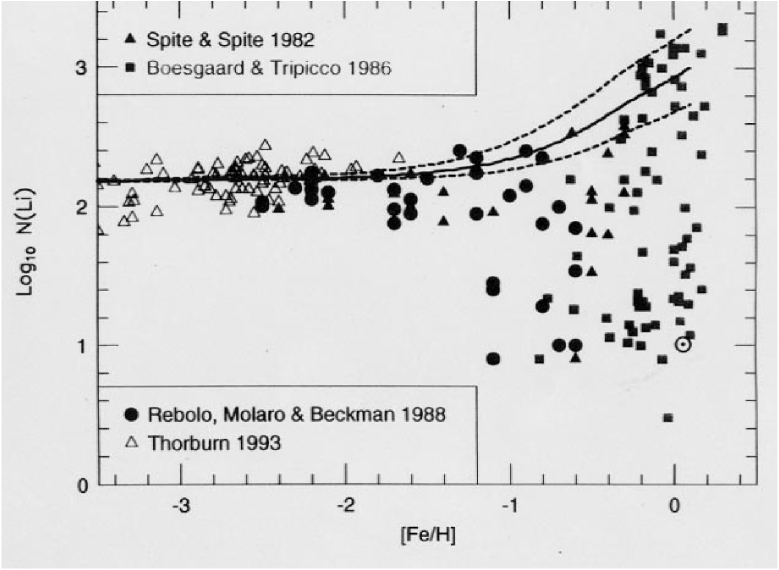
Figure 8: A compilation of the lithium abundance data from stellar observations as a function of metallicity. N(Li) $\equiv 10^{12}$(Li/H) and [Fe/H] is the usual metallicity relative to solar. Note the “Spite Plateau” in Li/H for [Fe/H] $\lower 2.58334pt\vbox{\hbox{$\buildrel\textstyle<\over{\sim}\ $}}-2$.

As with the other relic nuclides, the dominant uncertainties in estimating the primordial abundance of ⁷Li are not statistical, they are systematic. Lithium is observed in the atmospheres of cool stars (see Lambert (2002) in these lectures). It is the metal-poor, Pop II halo stars that are of direct relevance for the BBN abundance of ⁷Li. Uncertainties in the lithium equivalent width measurements, in the temperature scales for these Pop II stars, and in their model atmospheres, dominate the overall error budget. For example, Ryan et al. (2000), using the Ryan, Norris & Beers (1999) data, infer [Li]${}_{\rm P}\equiv 12+$log(Li/H)$=2.1$, while Bonifacio & Molaro (1997) and Bonifacio, Molaro & Pasquini (1997) derive [Li]${}_{\rm P}=2.2$, and Thorburn (1994) finds [Li]${}_{\rm P}=2.3$. From recent observations of stars in a metal-poor globular cluster, Bonifacio et al. (2002) derive [Li]${}_{\rm P}=2.34\pm 0.056$. But, there’s more.

The very metal-poor halo stars used to define the lithium plateau are very old. They have had the most time to disturb the prestellar lithium which may survive in their cooler, outer layers. Mixing of these outer layers with the hotter interior where lithium has been destroyed will dilute the surface abundance. Pinsonneault et al. (1999, 2002) have shown that rotational mixing may decrease the surface abundance of lithium in these Pop II stars by 0.1 – 0.3 dex while maintaining a rather narrow dispersion among their abundances (see also, Chaboyer et al. 1992; Theado & Vauclair 2001, Salaris & Weiss 2002).

In Pinsonneault et al. (2002) we adopted for our baseline (Spite Plateau) estimate [Li]$=2.2\pm 0.1$; for an overall depletion factor we chose 0.2 $\pm 0.1$ dex. Combining these linearly, we derived an estimate of the primordial lithium abundance of [Li]${}_{\rm P}=2.4\pm 0.2$. I will use this in the comparison between theory and observation to be addressed next.

4 Confrontation Of Theoretical Predictions With Observational Data

As the discussion in the previous section should have made clear, the attempts to use a variety of observational data to infer the BBN abundances of the light nuclides is fraught with evolutionary uncertainties and dominated by systematic errors. It may be folly to represent such data by a “best” value along with normally distributed errors. Nonetheless, in the absence of a better alternative, this is what will be done in the following.

• Deuterium

  From their data along the lines-of-sight to three QSOALS, O’Meara et al. (2001) recommend (D/H)${}_{\rm P}=3.0\pm 0.4\times 10^{-5}$. While I agree this is likely a good estimate for the central value, the spread among the extant data (see Figures 3 – 5) favors a larger uncertainty. Since D is only destroyed in the post-BBN universe, the solar system and ISM abundances set a floor to the primordial value. Keeping this in mind, I will adopt asymmetric errors ($\sim 1\sigma$): (D/H)${}_{\rm P}=3.0^{+1.0}_{-0.5}\times 10^{-5}$.

• Helium-4

  In our discussion of ⁴He as derived from hydrogen and helium recombination lines in low-metallicity, extragalactic H $\scriptstyle{\rm II}$ regions it was noted that the inferred primordial mass fraction varied from Y${}_{\rm P}=0.234\pm 0.003$ (OS/OSS), to Y${}_{\rm P}=0.238\pm 0.003$ (PPL and GSV), to Y${}_{\rm P}=0.244\pm 0.002$ (IT/ITL). Following the recommendation of OSW, here I will choose as a compromise Y${}_{\rm P}=0.238\pm 0.005$.

• Lithium-7

  Here, too, the spread in the level of the “Spite Plateau” dominates the formal errors in the means among the different data sets. To this must be added the uncertainties due to temperature scale and model atmospheres, as well as some allowance for dilution or depletion over the long lifetimes of the metal-poor halo stars. Attempting to accomodate all these sources of systematic uncertainty, I adopt the Pinsonneault et al. (2002) choice of [Li]${}_{\rm P}=2.4\pm 0.2$.

As discussed earlier, the stellar and Galactic chemical evolution uncertainties afflicting ³He are so large as to render the use of ³He to probe or test BBN problematic; therefore, I will ignore ³He in the subsequent discussion. There are a variety of equally valid approaches to using D, ⁴He, and ⁷Li to test and constrain the standard models of cosmology and particle physics (SBBN). In the approach adopted here deuterium will be used to constrain the baryon density ($\eta$ or, equivalently, $\Omega_{\rm B}h^{2}\;$). Within SBBN, this leads to predictions of Y_P and [Li]_P. Indeed, once the primordial deuterium abundance is chosen, $\eta$ may be eliminated and both Y_P and [Li]_P predicted directly, thereby testing the consistency of SBBN.

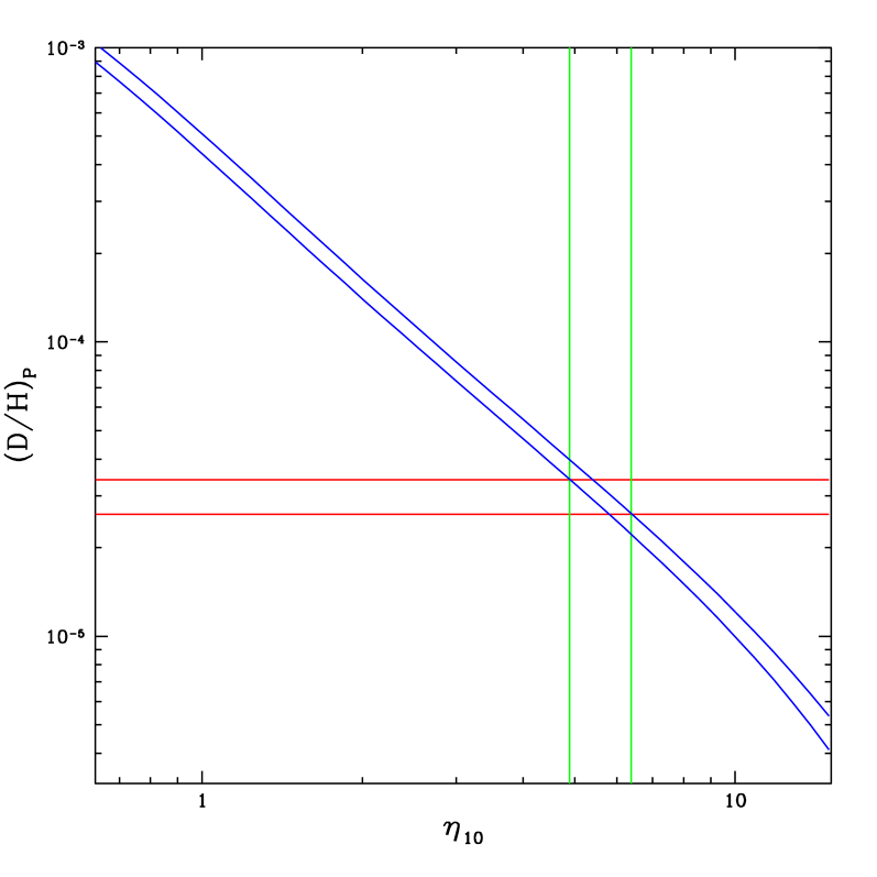
Figure 9: The diagonal band is the SBBN-predicted deuterium abundance (by number relative to hydrogen) as a function of the nucleon-to-photon ratio $\eta_{10}$ (the width of the band accounts for the theoretical uncertainties in the SBBN prediction). The horizontal band is the $\pm 1\sigma$ range in the adopted primordial deuterium abundance. The vertical band is, approximately, the corresponding SBBN-predicted $\eta$ range.

4.1 Deuterium – The Baryometer Of Choice

Recall that D is produced (in an astrophysically interesting abundance) ONLY during BBN. The predicted primordial abundance is sensitive to the baryon density (D/H  $\propto\eta^{-1.6}$). Furthermore, during post-BBN evolution, as gas is cycled through stars, deuterium is ONLY destroyed, so that for the “true” abundance of D anywhere, at any time, (D/H)${}_{\rm P}\geq({\rm D}/{\rm H})_{\rm TRUE}$. That’s the good news. The bad news is that the spectra of H $\scriptstyle{\rm I}$ and D $\scriptstyle{\rm I}$ are identical, except for the wavelength/velocity shift in their spectral lines. As a result, the true D-abundance may differ from that inferred from the observations if some of the presumed D $\scriptstyle{\rm I}$ is actually an H $\scriptstyle{\rm I}$ interloper masquerading as D $\scriptstyle{\rm I}$: (D/H)${}_{\rm TRUE}\leq({\rm D}/{\rm H})_{\rm OBS}$. Because of these opposing effects, the connection between (D/H)_OBS and (D/H)_P is not predetermined; the data themselves which must tell us how to relate the two. With this caveat in mind, it will be assumed that the value of (D/H)_P identified above is a fair estimate of the primordial D abundance. Using it, the SBBN-predicted baryon abundance may be determined. The result of this comparison is shown in Figure 9 where, approximately, the overlap between the SBBN-predicted band and that from the data fix the allowed range of $\eta$.

4.2 SBBN Baryon Density – The Baryon Density At 20 Minutes

The universal abundance of baryons which follows from SBBN and our adopted primordial D-abundance is: $\eta_{10}=5.6^{+0.6}_{-1.2}$ ($\Omega_{\rm B}h^{2}\;$$=0.020^{+0.002}_{-0.004}$). For the HST Key Project recommended value for $H_{0}$ ($h=0.72\pm 0.08$; Freedman et al. 2001), the fraction of the present universe critical density contributed by baryons is small, $\Omega_{\rm B}\approx 0.04$. In Figure 10 is shown a comparison among the various determinations of the present mass/energy density (as a fraction of the critical density), baryonic as well as non-baryonic. It is clear from Figure 10 that the present universe ($z~{}\lower 2.58334pt\vbox{\hbox{$\buildrel\textstyle<\over{\sim}\ $}}1$) baryon density inferred from SBBN far exceeds that inferred from emission/absorption observations (Persic & Salucci 1992, Fukugita, Hogan & Peebles 1998). The gap between the upper bound to luminous baryons and the BBN band is the “dark baryon problem”: at present, most of the baryons in the universe are dark. Evidence that although dark, the baryons are, indeed, present comes from the absorption observed in the Ly$\alpha$ forest at redshifts $z\approx 2-3$ (see, e.g., Weinberg et al. 1997). The gap between the BBN band and the band labelled by $\Omega_{\rm M}$ is the “dark matter problem”: the mass density inferred from the structure and movements of the galaxies and galaxy clusters far exceeds the SBBN baryon contribution. Most of the mass in the universe must be nonbaryonic. Finally, the gap from the top of the $\Omega_{\rm M}$ band to $\Omega=1$ is the “dark energy problem”.

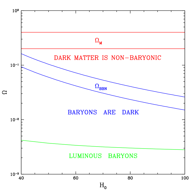
Figure 10: The various contributions to the present universal mass/energy density, as a fraction of the critical density ($\Omega$), as a function of the Hubble parameter ($H_{0}$). The curve labelled Luminous Baryons is an estimate of the upper bound to those baryons seen at present ($z~{}\lower 2.58334pt\vbox{\hbox{$\buildrel\textstyle<\over{\sim}\ $}}1$) either in emission or absorption (see the text). The band labelled BBN represents the D-predicted SBBN baryon density. The band labelled by “M” ($\Omega_{\rm M}=0.3\pm 0.1$) is an estimate of the current mass density in nonrelativistic particles (“Dark Matter”).

4.3 CMB Baryon Density – The Baryon Density At A Few Hundred Thousand Years

As discussed in the first lecture, the early universe is hot and dominated by relativistic particles (“radiation”). As the universe expands and cools, nonrelativistic particles (“matter”) come to dominate after a few hundred thousand years, and any preexisting density perturbations can begin to grow under the influence of gravity. On length scales determined by the density of baryons, oscillations (“sound waves”) in the baryon-photon fluid develop. At a redshift of $z\sim 1100$ the electron-proton plasma combines (“recombination) to form neutral hydrogen which is transparent to the CMB photons. Free to travel throughout the post-recombination universe, these CMB photons preserve the record of the baryon-photon oscillations as small temperature fluctuations in the CMB spectrum. Utilizing recent CMB observations (Lee et al. 2001; Netterfield et al. 2002; Halverson et al. 2002), many groups have inferred the intermediate age universe baryon density. The work of our group at OSU (Kneller et al. 2002) is consistent with more detailed analyses and is the one I adopt for the purpose of comparison with the SBBN result: $\eta_{10}=6.0\pm 0.6$; $\Omega_{\rm B}h^{2}\;$$=0.022\pm 0.002$.

4.4 The Baryon Density At 10 Gyr

Although the majority of baryons in the recent/present universe are dark, it is still possible to constrain the baryon density indirectly using observational data (see, e.g., Steigman, Hata & Felten 1999, Steigman, Walker & Zentner 2000; Steigman 2001). The magnitude-redshift relation determined by observations of type Ia supernovae (SNIa) constrain the relation between the present matter density ($\Omega_{\rm M}$) and that in a cosmological constant ($\Omega_{\Lambda}$). The allowed region in the $\Omega_{\Lambda}$ – $\Omega_{\rm M}$ plane derived from the observations of Perlmutter et al. (1997), Schmidt et al. (1998), and Perlmutter et al. (1999) are shown in Figure 11.

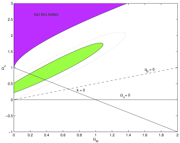
Figure 11: The 68% (solid) and 95% (dotted) contours in the $\Omega_{\Lambda}$ – $\Omega_{\rm M}$ plane consistent with the SNIa data (see the text). Geometrically flat models lie along the line labelled k = 0.

If, in addition, it is assumed that the universe is flat ($\kappa=0$; an assumption supported by the CMB data), a reasonably accurate determination of $\Omega_{\rm M}$ results: $\Omega_{\rm M}({\rm SNIa;Flat})=0.28^{+0.08}_{-0.07}$ (Steigman, Walker & Zentner 2000; Steigman 2001). But, how to go from the matter density to the baryon density? For this we utilize rich clusters of galaxies, the largest collapsed objects, which provide an ideal probe of the baryon fraction in the present universe $f_{\rm B}$. X-ray observations of the hot gas in clusters, when corrected for the baryons in stars (albeit not for any dark cluster baryons), can be used to estimate $f_{\rm B}$. Using the Grego et al. (2001) observations of the Sunyaev-Zeldovich effect in clusters, Steigman, Kneller & Zentner (2002) estimate $f_{\rm B}$ and derive a present-universe ($t_{0}\approx 10$ Gyr; $z~{}\lower 2.58334pt\vbox{\hbox{$\buildrel\textstyle<\over{\sim}\ $}}1$) baryon density: $\eta_{10}=5.1^{+1.8}_{-1.4}$ ($\Omega_{\rm B}h^{2}\;$$=0.019^{+0.007}_{-0.005}$).

4.5 Baryon Density Concordance

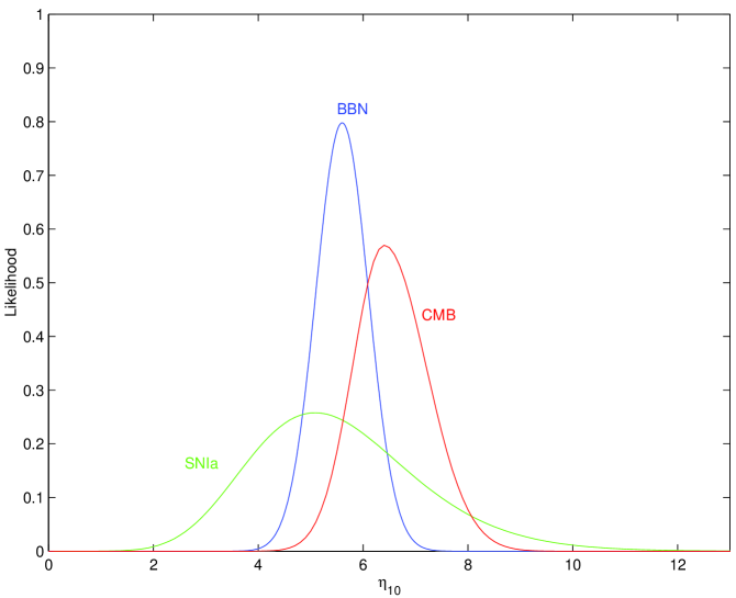
Figure 12: The likelihood distributions, normalized to equal areas under the curves, for the baryon-to-photon ratios ($\eta_{10}$) derived from BBN ($\sim 20$ minutes), from the CMB ($\sim$ few hundred thousand years), and for the present universe ($t_{0}\sim 10$ Gyr; $z~{}\lower 2.58334pt\vbox{\hbox{$\buildrel\textstyle<\over{\sim}\ $}}1$).

In Figure 12 are shown the likelihood distributions for the three baryon density determinations discussed above. It is clear that these disparate determinations, relying on completely different physics and from widely separated epochs in the evolution of the universe are in excellent agreement, providing strong support for the standard, hot big bang cosmological model and for the standard model of particle physics. Although it has been emphasized many times in these lectures that the errors are likely dominated by evolutionary and systematic uncertainties and, therefore, are almost certainly not normally distributed, it is hard to avoid the temptation to combine these three independent estimates. Succumbing to temptation: $\eta_{10}=5.8^{+0.4}_{-0.6}$ ($\Omega_{\rm B}h^{2}\;$ $=0.021^{+0.0015}_{-0.0020}$).

4.6 Testing The Consistency Of SBBN

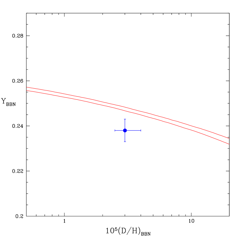
Figure 13: The diagonal band is the SBBN-predicted helium-4 mass fraction versus the SBBN-predicted deuterium abundance (by number relative to hydrogen). The width of the band accounts for the theoretical uncertainties in the SBBN predictions. Also shown by the filled circle and error bars are the primordial ⁴He and D abundance estimates adopted here.

As impressive as is the agreement among the three independent estimates of the universal baryon density, we should not be lured into complacency. The apparent success of SBBN should impell us to test the standard model even further. How else to expose possible systematic errors which have heretofore been hidden from view or, to find the path beyond the standard models of cosmology and particle physics? To this end, in Figure 13 are compared the SBBN ⁴He (Y) and D (D/H) abundance predictions along with the estimates for Y and D/H adopted here. The agreement is not very good. Indeed, while for $\eta_{10}=5.8^{+0.4}_{-0.6}$, (D/H)${}_{\rm SBBN}=2.8^{+0.4}_{-0.7}\times 10^{-5}$, in excellent agreement with the O’Meara et al. (2001) estimate, the corresponding ⁴He abundance is predicted to be Y${}_{\rm SBBN}=0.248\pm 0.001$, which is 2$\sigma$ above our OSW-adopted primordial abundance. Indeed, the SBBN-predicted ⁴He abundance based directly on deuterium is also $2\sigma$ above the IT/ITL estimate. Here is a potential challenge to the internal consistency of SBBN. Given that systematic errors dominate, it is difficult to decide how seriously to take this challenge. In fact, if ⁴He and D, in concert with SBBN, are each employed as baryometers, their likelihood distributions for $\eta$ are consistent at the 7% level.

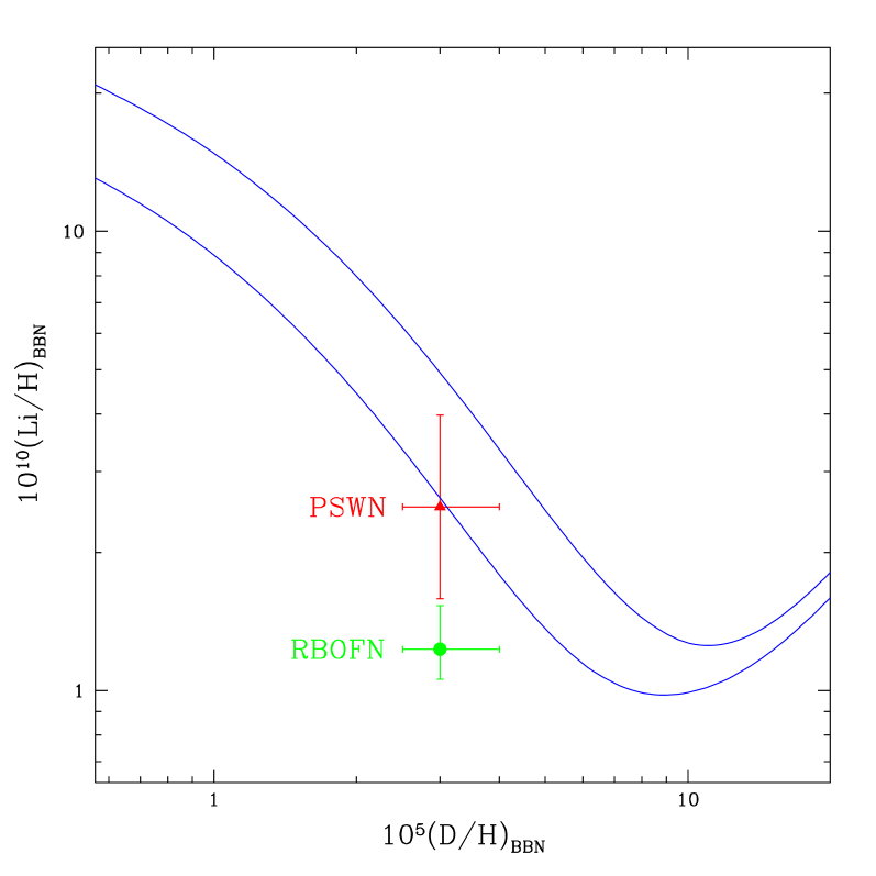
Figure 14: The band is the SBBN-predicted lithium abundance (by number relative to hydrogen) versus the SBBN-predicted deuterium abundance. The width of the band accounts for the theoretical uncertainties in the SBBN predictions. Also shown is the Pinsonneault et al. (2002; PSWN) primordial lithium abundance estimate adopted here (filled triangle) along with the Ryan et al. (2000; RBOFN) estimate (filled circle).

An apparent success of (or, a potential challenge to) SBBN emerges from a comparison between D and ⁷Li. In Figure 14 is shown the SBBN-predicted relation between primordial D and primordial ⁷Li along with the relic abundance estimates adopted here (Pinsonneault et al. 2002). Also shown for comparison is the Ryan et al. (2000) primordial lithium abundance estimate. The higher, depletion/dilution-corrected lithium abundance of PSWN is in excellent agreement with the SBBN-D abundance, while the lower, RBOFN value poses a challenge to SBBN.

5 BBN In Non-Standard Models

As just discussed in §4.6, there is some tension between the SBBN-predicted abundances of D and ⁴He and their primordial abundances inferred from current observational data (see Fig. 13). Another way to see the challenge is to superpose the data on the BBN predictions from Figure 2, where the Y_P versus D/H relations are shown for several values of N_ν (SSG). This is done in Figure 15 where it is clear that the data prefer nonstandard BBN, with N_ν closer to 2 than to the standard model value of 3.

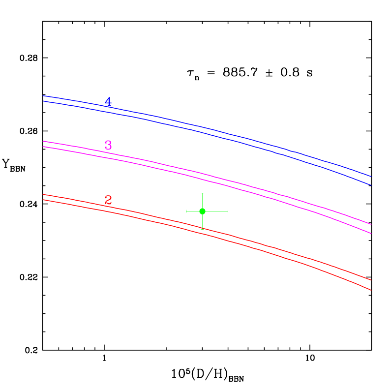
Figure 15: The BBN-predicted primordial ⁴He mass fraction Y as a function of the BBN-predicted primordial Deuterium abundance (by number relative to Hydrogen) for three choices of N_ν. Also shown by the filled circle and error bars are the primordial abundances adopted here (§4).

It is easy to understand this result on the basis of the earlier discussion (see §2.3). The adopted abundance of D serves, mainly, to fix the baryon density which, in turn, determines the SBBN-predicted ⁴He abundance. The corresponding predicted value of Y_P is too large when compared to the data. A universe which expands more slowly ($S<1$; N${}_{\nu}<3$) will permit more neutrons to transmute into protons before BBN commences, resulting in a smaller ⁴He mass fraction. However, there are two problems (at least!) with this “solution”. The main issue is that there are three “flavors” of light neutrinos, so that N${}_{\nu}\geq 3$ ($\Delta$N${}_{\nu}\geq 0$). The second, probably less serious problem is that a slower expansion permits an increase in the ⁷Be production, resulting in an increase in the predicted relic abundance of lithium. For (D/H)${}_{\rm P}=3.0\times 10^{-5}$ and Y_P = 0.238, the best fit values of $\eta$ and $\Delta N_{\nu}\;$are: $\eta_{10}=5.3$ ($\Omega_{\rm B}h^{2}\;$= 0.019) and N${}_{\nu}=2.3$ ($\Delta N_{\nu}\;$$=-0.7$). For this combination the BBN-predicted lithium abundance is [Li]${}_{\rm P}=2.53$ ((Li/H)${}_{\rm P}=3.4\times 10^{-10}$), somewhat higher than, but still in agreement with the PSWN estimate of [Li]${}_{\rm P}=2.4\pm 0.2$, but much higher than the RBOFN value of [Li]${}_{\rm P}=2.1\pm 0.1$. Although the tension between the observed and SBBN-predicted lithium abundances may not represent a serious challenge (at present), the suggestion that $\Delta N_{\nu}\;$$<0$ must be addressed. One possibility is that the slower expansion of the radiation-domianted early universe could result from a non-minimally coupled scalar field (“extended quintessence”) whose effect is to change the effective gravitational constant ($G\rightarrow G^{\prime}<G$; see §2.3). For a discussion of such models and for further references see, e.g., Chen, Scherrer & Steigman (2001).

5.1 Degenerate BBN

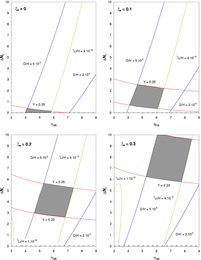
Figure 16: Isoabundance contours for D, ⁴He, and ⁷Li in the $\Delta N_{\nu}\;$– $\eta_{10}$ plane for four choices of the $\nu_{e}$ degeneracy parameter $\xi_{e}$. The shaded areas identify the ranges of parameters consistent with the abundances indicated (see the text).

There is another alternative to SBBN which, although currently less favored, does have a venerable history: BBN in the presence of a background of degenerate neutrinos. First, a brief diversion to provide some perspective. In the very early universe there were a large number of particle-antiparticle pairs of all kinds. As the baryon-antibaryon pairs or, their quark-antiquark precursors, annihilated, only the baryon excess survived. This baryon number excess, proportional to $\eta$, is very small ($\eta~{}\lower 2.58334pt\vbox{\hbox{$\buildrel\textstyle<\over{\sim}\ $}}10^{-9}$). It is reasonable, but by no means compulsory, to assume that the lepton number asymmetry (between leptons and antileptons) is also very small. Charge neutrality of the universe ensures that the electron asymmetry is of the same order as the baryon asymmetry. But, what of the asymmetry among the several neutrino flavors?

Since the relic neutrino background has never been observed directly, not much can be said about its asymmetry. However, if there is an excess in the number of neutrinos compared to antineutrinos (or, vice-versa), “neutrino degeneracy”, the total energy density in neutrinos (plus antineutrinos) is increased. As a result, during the early, radiation-dominated evolution of the universe, $\rho\rightarrow\rho^{\prime}>\rho$, and the universal expansion rate increases ($S>1$). Constraints on how large $S$ can be do lead to some weak bounds on neutrino degeneracy (see, e.g., Kang & Steigman 1992 and references therein). This effect occurs for degeneracy in all neutrino flavors ($\nu_{e}$, $\nu_{\mu}$, and $\nu_{\tau}$). For fixed baryon density, $S>1$ leads to an increase in D/H (less time to destroy D), more ⁴He (less time to transform neutrons into protons), and a decrease in lithium (at high $\eta$ there is less time to produce ⁷Be). Recall that for $S=1$ (SBBN), an increase in $\eta$ results in less D (more rapid destruction), which can compensate for $S>1$. Similarly, an increase in baryon density will increase the lithium yield (more rapid production of ⁷Be), also tending to compensate for $S>1$. But, at higher $\eta$, more ⁴He is produced, further exacerbating the effect of a more rapidly expanding universe.

However, electron-type neutrinos play a unique role in BBN, mediating the neutron-proton transformations via the weak interactions (see eq. 2.24). Suppose, for example, there are more $\nu_{e}$ than $\bar{\nu}_{e}$. If $\mu_{e}$ is the $\nu_{e}$ chemical potential, then $\xi_{e}\equiv\mu_{e}/kT$ is the “neutrino degeneracy parameter”; in this case, $\xi_{e}>0$. The excess of $\nu_{e}$ will drive down the neutron-to-proton ratio, leading to a reduction in the primordial ⁴He mass fraction. Thus, a combination of three adjustable parameters, $\eta$, $\Delta$N_ν, and $\xi_{e}$ may be varied to “tune” the primordial abundances of D, ⁴He, and ⁷Li. In Kneller et al. (2001; KSSW), we chose a range of primordial abundances similar to those adopted here ($2\leq 10^{5}$(D/H)${}_{\rm P}\leq 5$; $0.23\leq$ Y${}_{\rm P}\leq 0.25$; $1\leq 10^{10}$(Li/H)${}_{\rm P}\leq 4$) and explored the consistent ranges of $\eta$, $\xi_{e}\geq 0$, and $\Delta$N${}_{\nu}\geq 0$. Our results are shown in Figure 16.

It is clear from Figure 16 that for a large range in $\eta$, a combination of $\Delta N_{\nu}\;$and $\xi_{e}$ can be found so that the BBN-predicted abundances will lie within our adopted primordial abundance ranges. However, there are constraints on $\eta$ and $\Delta N_{\nu}\;$from the CMB temperature fluctuation spectrum (see KSSW for details and further references). Although the CMB temperature fluctuation spectrum is insensitive to $\xi_{e}$, it will be modified by any changes in the universal expansion rate. While SBBN ($\Delta N_{\nu}\;$= 0) is consistent with the combined constraints from BBN and the CMB (see §4.5) for $\eta_{10}\approx 5.8$ ($\Omega_{\rm B}h^{2}\;$$\approx 0.021$), values of $\Delta N_{\nu}\;$as large as $\Delta N_{\nu}\;$$\lower 2.58334pt\vbox{\hbox{$\buildrel\textstyle<\over{\sim}\ $}}6$ are also allowed (KSSW).

6 Summary

As observations reveal, the present universe is filled with radiation and is expanding. According to the standard, hot big bang cosmological model the early universe was hot and dense and, during the first few minutes in its evolution, was a primordial nuclear reactor, synthesizing in significant abundances the light nuclides D, ³He, ⁴He, and ⁷Li. These relics from the Big Bang open a window on the early evolution of the universe and provide probes of the standard models of cosmology and of particle physics. Since the BBN-predicted abundances depend on the competition between the early universe expansion rate and the weak- and nuclear-interaction rates, they can be used to test the standard models as well as to constrain the universal abundances of baryons and neutrinos. This enterprise engages astronomers, astrophysicists, cosmologists, and particle physicists alike. A wealth of new observational data has reinvigorated this subject and stimulated much recent activity. Much has been learned, revealing many new avenues to be explored (a key message for the students at this school – and for young researchers everywhere). The current high level of activity ensures that many of the detailed, quantitative results presented in these lectures will need to be revised in the light of new data, new analyses of extant data, and new theoretical ideas. Nonetheless, the underlying physics and the approaches to confronting the theoretical predictions with the observational data presented in these lectures should provide a firm foundation for future progress.

Within the context of the standard models of cosmology and of particle physics (SBBN) the relic abundances of the light nuclides depend on only one free parameter, the baryon-to-photon ratio (or, equivalently, the present-universe baryon density parameter). With one adjustable parameter and three relic abundances (four if ³He is included), SBBN is an overdetermined theory, potentially falsifiable. The current status of the comparison between predictions and observations reviewed here illuminates the brilliant success of the standard models. Among the relic light nuclides, deuterium is the baryometer of choice. For N${}_{\nu}=3$, the SBBN-predicted deuterium abundance agrees with the primordial-D abundance derived from the current observational data for $\eta_{10}=5.6^{+0.6}_{-1.2}$ ($\Omega_{\rm B}=0.020^{+0.002}_{-0.004}$). This baryon abundance, from the first 20 minutes of the evolution of the universe, is in excellent agreement with independent determinations from the CMB ($\sim$ few hundred thousand years) and in the present universe ($\sim$ 10 Gyr).

It is premature, however, to draw the conclusion that the present status of the comparison between theory and data closes the door on further interesting theoretical and/or observational work. As discussed in these lectures, there is some tension between the SBBN-predicted abundances and the relic abundances derived from the observational data. For the deuterium-inferred SBBN baryon density, the expected relic abundances of ⁴He and ⁷Li are somewhat higher than those derived from current data. The “problems” may lie with the data (large enough data sets? underestimated errors?) or, with the path from the data to the relic abundances (systematic errors? evolutionary corrections?). For example, has an overlooked correction to the H $\scriptstyle{\rm II}$ region-derived ⁴He abundances resulted in a value of Y_P which is systematically too small (e.g., underlying stellar absorption)? Are there systematic errors in the absolute level of the lithium abundance on the Spite Plateau or, has the correction for depletion/dilution been underestimated? In these lectures the possibility that the fault may lie with the cosmology was also explored. In one simple extension of SBBN, the early universe expansion rate is allowed to differ from that in the standard model. It was noted that to reconcile D, and ⁴He would require a slower than standard expansion rate, difficult to reconcile with simple particle physics extensions beyond the standard model. Furthermore, if this should be the resolution of the tension between D and ⁴He, it would exacerbate that between the predicted and observed lithium abundances. The three abundances could be reconciled in a further extension involving neutrino degeneracy (an asymmetry between electron neutrinos and their antiparticles). But, three adjustable parameters to account for three relic abundances is far from satisfying. Clearly, this active and exciting area of current research still has some surprises in store, waiting to be discovered by astronomers, astrophysicists, cosmologists and particle physicists. The message to the students at this school – and those everywhere – is that much interesting observational and theoretical work remains to be done. I therefore conclude these lectures with a personal list of questions I would like to see addressed.

• Where (at what value of D/H) is the primordial deuterium plateau, and what is(are) the reason(s) for the currently observed spread among the high-$z$, low-Z QSOALS D-abundances?

• Are there stellar observations which could offer complementary insights to those from H $\scriptstyle{\rm II}$ regions on the question of the primordial ⁴He abundance, perhaps revealing unidentified or unquantified systematic errors in the latter approach? Is Y_P closer to 0.24 or 0.25?

• What is the level of the Spite Plateau lithium abundance? Which observations can pin down the systematic corrections due to model stellar atmospheres and temperature scales and which may reveal evidence for, and quantify, early-Galaxy production as well as stellar depletion/destruction?

• If further observational and associated theoretical work should confirm the current tension among the SBBN-predicted and observed primordial abundances of D, ⁴He, ⁷Li, what physics beyond the standard models of cosmology and particle physics has the potential to resolve the apparent conflicts? Are those models which modify the early, radiation-dominated universe expansion rate consistent with observations of the CMB temperature fluctuation spectrum? If neutrino degeneracy is invoked, is it consistent with the neutrino properties (masses and mixing angles) inferred from laboratory experiments as well as the solar and cosmic ray neutrino oscallation data?

To paraphrase Spock, work long and prosper!