Data reduction and astrometry strategies for wide-field images: an application to the Capodimonte Deep Field

Abstract

The Capodimonte Deep Field (OACDF) is a multi-colour imaging survey on two 0.5x0.5 square degree fields performed in the BVRI bands and in six medium-band filters (700 - 900 nm) with the Wide Field Imager (WFI) at the ESO 2.2 m telescope at La Silla, Chile. In this contribution the adopted strategies for the OACDF data reduction are discussed. Preliminary scientific results of the survey are also presented.

1 Introduction

In view of the arrival of the VLT Survey Telescope (VST) (a cooperation of ESO, the Capodimonte Astronomical Observatory-OAC-Naples, Italy, and the European Consortium Omegacam, for the design, realization, installation, and operation at ESO Paranal Observatory in Chile of a 2.6 m aperture, 1 degree x 1 degree wide field imaging facility in the spectral range from UV to I bands), the OAC started a pilot project, called the Capodimonte Deep Field (OACDF), consisting in a multi-colour imaging survey using the Wide Field Imager (WFI, Baade et al. 1998 ) at the ESO 2.2 m telescope at La Silla, Chile. The VST will be equipped with OmegaCam, a 16k X 16k array of 32 CCDs, which will cover 1 square degree. The main goal of the OACDF is to provide a large photometric database, mainly oriented to extragalactic studies (quasars, high-redshift galaxies, galaxy counts, lensing, etc.), that can be used also for stellar and planetary research (galactic halo population, peculiar objects like brown dwarfs and cool white dwarfs, Kuiper-Belt objects). Another goal is to gain insight into the handling and processing of data coming from a wide field imager, similar to the one which will be installed at VST.

In this contribution we discuss technical aspects of the OACDF data reduction and present some preliminary scientific results. We focus on the following topics: super flat-fielding and defringing of the mosaics, astrometry and photometric calibration. Such topics will be of primary importance for the processing of the VLT Survey Telescope (VST) data, in the framework of the European consortium ASTRO-WISE (see http://www.ASTRO-WISE.org). Some of the problems encountered are intrinsic to the ESO WFI. Hence, our tests might contribute to a better characterisation of this instrument. In addition, we report on some preliminary scientific results of the OACDF project. The depth of the OACDF (25.1 mag in the R band) allows to achieve the foreseen scientific goals: i) the search for rare/peculiar objects, AGNs and high-redshift QSO’s (z$>$3); ii) the search for intermediate-redshift early-type galaxies to be used as tracers of galaxy evolution and iii) the search for galaxy clusters to be used as targets for spectroscopic follow-up’s at larger telescopes.

2 Observations

The observations for the OACDF project were performed in three different periods (18–22 April 1999, 7–12 March 2000 and 26–30 April 2000) using the WFI mosaic camera attached to the ESO 2.2m telescope at La Silla, Chile. This camera consists of eight 2k$\times$4k CCDs that constitute a 8k$\times$8k array. The scale is $0.238^{\prime\prime}$/pix. Some 100 Gbyte of raw data were collected in each one of the three observing runs. The first and third run were photometric, while the second one was partially non-photometric.

The observational strategy was to perform a 1 deg² shallow survey and a 0.5 deg² deep survey. The shallow survey was performed in the B,V,R and I broad-band filters. Four adjacent $30^{\prime}\times 30^{\prime}$ fields, covering a $1^{\circ}\times 1^{\circ}$ field in the sky, were observed for the shallow survey. We call these fields OACDF1, OACDF2, OACDF3 and OACDF4. The OACDF2 and OACDF4 were chosen for the 0.5 deg² deep survey. The deep survey was performed in the B,V,R broad-bands and in six medium-band filters (700 - 900 nm).

Several standard fields, selected from the Landolt (1992) E-regions were observed in order to transform the BVRI instrumental magnitudes to the standard Johnson/Kron-Cousins system. Likewise, several spectrophotometric standard stars were observed in the intermediate-band filters for absolute flux calibration purposes.

Being obtained with a mosaic imager, the WFI data are multi-extension fits files (MEFs). Each extension corresponds to one of the eight CCDs of the mosaic. The physical separation of each one of the CCDs with respect to each other is about 100$\mu$. A sequence of ditherings following a rhombi-like pattern were performed in order to cover the CCD gaps. For the shallow survey a sequence of 5 ditherings was done, while at least 8 ditherings were done for the deep survey.

3 Data reduction

A two-processor (with 500 Mhz each) DS20 machine with hundred Gbyte of hard disk was used for the data reduction. The mscred task under IRAF was used to perform the data reduction. The reduction steps are described next.

3.1 Bias and dark

A mean Bias was created nightly. The bias subtraction was performed extension by extension. Several sixty-minute dark exposures were used to derive average dark frames for each night. No significant contribution from the mean dark to the noise was found.

3.2 Flat-fielding

A nightly super-flat was created as the result of the median of all the science frames taken in the same filter. We define $supFlat=\langle science~{}frames\rangle$. By means of a rejection algorithm, all astronomical sources over the background level, as well as cosmic particle heats and bad columns are normally removed in the resulting $supFlat$ image, because of the dithering pattern.

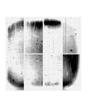
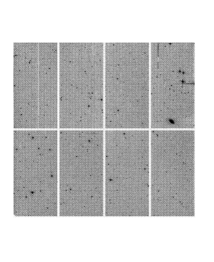
Figure 1: Raw (left) vs. pre-reduced (right) OACDF image in the R band. The exposure time of this image is 900 seconds.

Several twilight sky exposures were used to create a mean nightly twilight sky-flat. We define $skyFlat=\langle skyFlats\rangle$. Rejection algorithms to remove objects and cosmic particle heats were also applied.

The nightly master-flat in each filter was created using as much information as possible from the twilight sky-flats and the super-flats: the $supFlat/skyFlat$ ratio gives the information on the difference between the twilight sky flats and the average science frame and hence, it provides the pattern due to large-scale non-uniform illumination which should be applied to flatten the science frames. The master-flat, $Flat$, is then obtained combining the mean sky-flat with the super-flat as follows:

$$Flat=smooth\Big{(}\frac{supFlat}{skyFlat}\Big{)}\cdot skyFlat$$ (1)

In this way, the super-flat is used to correct the large scale variations due to non-uniform illumination and the high S/N sky-flat is used to correct the high-frequency pixel-to-pixel sensitivity variations.

3.3 Fringing correction

A fringing pattern was derived first using the ratio $supFlat/skyFlat$ defined above. In case of images with fringing such ratio is a superposition of the fringing pattern, $frP$, itself and the background. For images without fringing, such background is the same as the ratio defined above. Therefore, in order to derive $frP$, it is sufficient to determine the background of the $supFlat/skyFlat$ ratio and subtract it from the ratio. Hence, the fringing pattern is given by:

$$frP=\frac{supFlat}{skyFlat}-backgr\_fit\Big{(}\frac{supFlat}{skyFlat}\Big{)}$$ (2)

The background fit gives us both the fringing pattern, from eq. 2, and the information for the non-uniform illumination correction, from the fit itself. Thus, the master-flat is determined using such fit in equation (1) instead of the smoothed ratio.

Once the raw images are debiassed, the flat-field and fringing correction are applied as follows:

$$PrI=\frac{Im}{Flat}-\eta\cdot frP$$ (3)

where $Im$ and $PrI$ are the debiased and pre-reduced image respectively. The factor $\eta$ is a function of the sky background and the air-mass which varies from one scientific image to the other. It has been found that adopting $\eta_{n}$ = bck_n / $<$bck$>$, where bck_n is the mean background of the n^th image and $<$bck$>$ is the mean background of the $supFlat/skyFlat$ ratio, gives good results. Typical values of $\eta$ run from 0.8 to 1.2. A fringing pattern was obtained for every set of ditherings in every filter of every OACDF observing run.

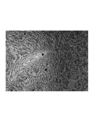
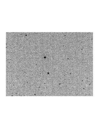
Figure 2: Section of an image of the CCD No. 6 in the $\lambda 816$-band with fringing (left). The final image, after correction by flatfield and fringing, is also shown (right).

Several tests were done in order to optimise the master flat. The resulting images are uniform to better than 1%. In Figure 1, the comparison between a raw and pre-reduced image in the R-band is shown. In Figure 2, a section of an image of the CCD No. 6 of the mosaic is shown before and after the fringing correction (left and right panels respectively).

3.4 The astrometry

Two different strategies may be adopted for the astrometric calibration:

1. For each dithering sequence a reference exposure is chosen: an astrometric solution is computed for the CCDs in this exposure with reference to an external astrometric catalog. The astrometry for the other exposures is then computed by fitting the positions of sources to those measured in the reference frame.

2. For all CCDs the astrometric solution is computed simultaneously using both the external astrometric catalog and the requirement that positions of sources overlapping in different CCDs are the same (global astrometry).

The first approach (see e.g. the mscred package in IRAF) works reasonably well in single pointings with compact dithers: however, it may give wrong results at the borders of the field, in particular if the offset between the exposures is large. In the case of the OACDF the covered field consists of multiple overlapping pointings and the offset between the exposures is typically $\geq$ 100 pixels. The global astrometry approach is therefore more convenient since it optimizes the internal astrometric accuracy. The usage of the USNO A2 as the astrometric catalog allows an RMS accuracy $\sim$ 0.3”; however the internal accuracy which may be obtained for overlapping sources in different bands is much lower. We therefore decided first to compute the astrometry for the R-band image taking the USNO A2 as reference: we obtain an RMS accuracy of $\sim$ 0.4” (see Figure 3). We then extracted a catalog of sources from the finally coadded image and used it as the astrometric catalog for the other bands. The RMS accuracy in this case is $\leq$ 0.13” (c.f. Figure 3).

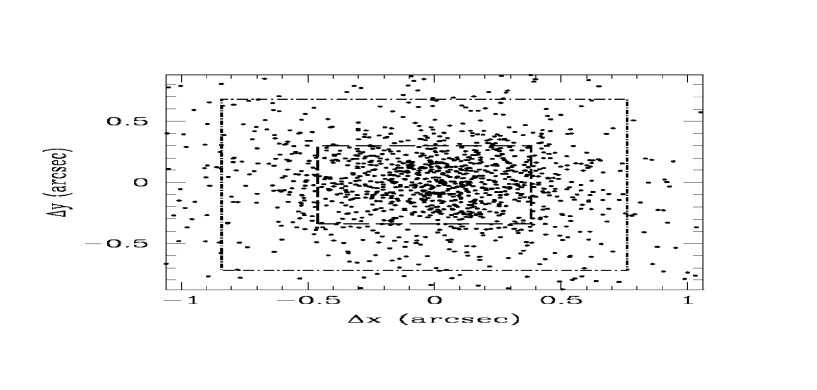
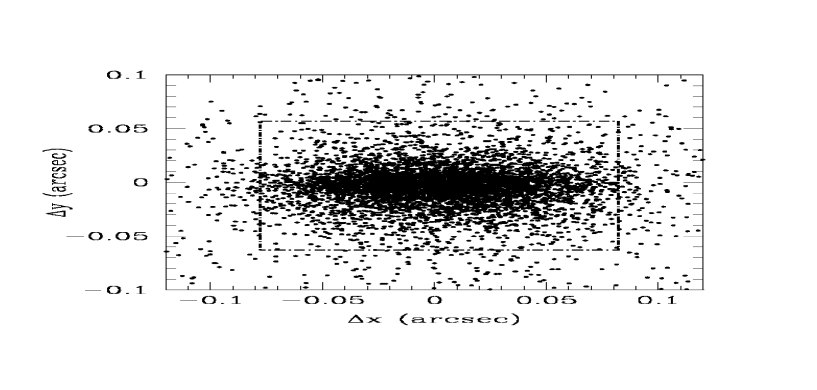
Figure 3: Astrometric residuals. Left: R vs. USNO; right: B vs. R. The dashed and dot-dashed lines show the residuals obtained for 68% and 95% of matched sources respectively.

The next step is to homogenize the internal photometry using an approach similar to that adopted for astrometry. The zero point for each frame is written as:

$$Z=Z_{ph}+Z_{r},$$ (4)

where $Z_{ph}$ is the photometric zero point computed from photometric standard fields (see later), $Z_{r}$ is an offset taking into account the changes in airmass, atmospheric conditions etc.. These offsets are computed requiring that overlapping sources in different exposures have the same flux. The photometry may be anchored to one or more ’photometric’ exposures for which $Z_{r}=0$.

Astrometry and photometry were computed using the ASTROMETRIX and PHOTOMETRIX tools developed by M.R. in the framework of a cooperation of OAC with the TERAPIX team (IAP, Paris). Both are freely available in http://www.na.astro.it/$\sim$radovich/wifix.htm.

Finally, images were resampled, scaled in flux and coadded using the SWarp tool developed by E. Bertin (http://terapix.iap.fr/soft/swarp).

4 The photometric calibration

4.1 The broad-band calibration

The B,V,R,I photometric calibrations were performed using the standard magnitudes and colours reported by Landolt (1992). For the Landolt-98 field, we used the larger set of photometric standards by Stetson (2000). The transformation equations are as follows:

$$B=b-k_{B}\cdot X+C_{B}\cdot(B-V)+Z_{B},$$ (5)

$$V=v-k_{V}\cdot X+C_{V}\cdot(B-V)+Z_{V},$$ (6)

$$R=r-k_{R}\cdot X+C_{R}\cdot(V-R)+Z_{R},$$ (7)

$$I=~{}i~{}-k_{I}\cdot X+C_{I}\cdot(V-I)+Z_{I},$$ (8)

where $X$ is the airmass, $b,v,r,i$ are the instrumental magnitudes, $k_{B},k_{V},k_{R},k_{I}$ the extinction coefficients, $C_{B},C_{V},C_{R},C_{I}$ the colour terms and $Z_{B},Z_{V},Z_{R},Z_{I}$ the zero points in the B,V,R,I bands respectively. The mean extinction coefficients for La Silla were adopted.

Some 100-200 standards were used for the linear fits. The fit residuals are typically less than 2%, but in some cases the residuals are as high as 5% . The relatively high residuals may be a consequence of the non-uniform illumination that will be discussed in Section 4.3. A few points with a particular high residual are due to stars falling partially in the CCD gaps and/or to photometric/astrometric errors in the standard catalogue. Such points were rejected by means of a sigma clipping algorithm.

More details on the broad-band photometric calibration will be published elsewhere.

4.2 The intermediate-band calibration

The flux calibration for the intermediate-band observations was performed using the observed spectrophotometric standard stars and following the prescription by Jacoby et al. (1987). For a given astronomical source, the absolute flux $F_{\lambda}$ measured at the earth in the band-width $\Delta\lambda$, is proportional to the extinction corrected count-rate measured in $\Delta\lambda$, and inversely proportional to the peak of the filter transmission. Let’s call the proportionality factor as the $"counts-to-energy"$ conversion factor $S_{\lambda}$. Thus,

$$F_{\lambda}=\frac{S_{\lambda}\cdot C_{\lambda}\cdot 10^{0.4\cdot k_{\lambda}\cdot X}}{T_{\lambda}}$$ (9)

where $C_{\lambda}$, $k_{\lambda}$, $X$ and $T_{\lambda}$ are the count-rate, the extinction coefficient, the airmass and the transmission peak in the band-width $\Delta\lambda$. The $"counts-to-energy"$ conversion factor $S_{\lambda}$ is a measure of the efficiency of the whole system (telescope + camera) and can be derived from the observations of different spectrophotometric standard stars. Using $n$ standard stars, one can compute a mean $S_{\lambda}=\sum_{i=1}^{n}S_{\lambda}(i)/n$. The $S_{\lambda}(i)$ factor can be determined from the count-rate $C_{\lambda}(i)$ of the $i^{th}$ standard star by convolving the spectral energy distribution, $F_{\lambda}(i)$, of the star with the filter transmission, $T_{\lambda}(i)$, using the following relation:

$$S_{\lambda}(i)=\frac{\int F_{\lambda}(i)\cdot T_{\lambda}d\lambda}{C_{\lambda}(i)\cdot 10^{0.4\cdot k_{\lambda}\cdot X(i)}}=\frac{F_{0}(i)\cdot\int T_{\lambda}d\lambda}{C_{\lambda}(i)\cdot 10^{0.4\cdot k_{\lambda}\cdot X(i)}}$$ (10)

The last step in the above equation is justified by the fact that the filters are narrow and the flux of the standard star can be considered as constant and equal to the value, $F_{0}$, in the center of the band. Since the factor $\int T_{\lambda}d\lambda$ gives the equivalent width, $W_{\lambda}$, of the filter, equation (10) can be written as follows:

$$S_{\lambda}(i)=\frac{F_{0}(i)\cdot W_{\lambda}}{C_{\lambda}(i)\cdot 10^{0.4\cdot k_{\lambda}\cdot X(i)}}$$ (11)

Therefore, the $S_{\lambda}$ factor is determined on the basis of the measured count-rate and the equivalent width of the filter. Adopting the extintion coefficients $k_{\lambda}=k_{I}$ = 0.08 for all the intermediate bands, and measuring the count-rate $C_{\lambda}(i)$ of each standard by means of apperture photometry, we obtained the $S_{\lambda}$ factors which are reported in Table 1 in units of 10${}^{-16}~{}erg\cdot s^{-1}\cdot cm^{-2}\cdot cts^{-1}$ Since the second observing run was partially non-photometric, the reported values are those for the first and third runs only.

Table 1: Mean $S_{\Delta\lambda}$ factors

Filter	run1	run3
(nm)
$\lambda$753	5.57$\pm$0.26	6.36$\pm$0.24
$\lambda$770	6.20$\pm$0.34	7.14$\pm$0.20
$\lambda$790	7.70$\pm$0.27	8.94$\pm$0.23
$\lambda$815	6.60$\pm$0.29	7.69$\pm$0.35
$\lambda$837	6.67$\pm$0.28	7.28$\pm$0.62
$\lambda$914	11.67$\pm$0.85	12.77$\pm$0.67

The AB magnitudes were determined from the relation: $m_{AB}(\nu)=-2.5\cdot(log(F_{\nu})+19.436)=-2.5\cdot log\Big{(}\frac{F_{\lambda}\cdot\lambda^{2}}{c}\Big{)}-48.59,$ where $c$ is the speed of light. From equation (11) and after some algebra, it can be shown that: $m_{AB}(\lambda)=-2.5\cdot log(C_{\lambda})+2.5\cdot log\Big{(}\frac{c\cdot W_{\lambda}}{S_{\lambda}\cdot\lambda^{2}}\Big{)}-k_{\lambda}\cdot X-48.59=m_{AB}(\lambda)=m_{inst}(\lambda)-k_{\lambda}\cdot X+Z_{\lambda}$ , where $Z_{\lambda}$ is the zero point defined as $Z_{\lambda}=2.5\cdot log\Big{(}\frac{c\cdot W_{\lambda}}{S_{\lambda}\cdot\lambda^{2}}\Big{)}-48.59$. In this way, the AB magnitudes can be determined for a given OACDF observation with airmass $X$ adopting the extinction coefficient $k_{\lambda}$. The airmass to be used here is the one correspondent to the OACDF observation taken as reference dithering for the determination of the scaling factors as explained in Section 3.4.

Figure 4: The relative photometric offsets versus the CCDs for the broad-band (left) and medium-band filters (right) is shown in the upper panles. The average over the filters is shown in the lower panels.

4.3 Inhomogeneity between different CCDs

In order to test the accuracy of the photometric calibrations over the whole mosaic, we observed a few selected standard fields in each of the eight CCDs.

For the broad-band, we used the Landolt field PG1525-071, which contains five stars with (B-V) colours in the range from -0.198 to 1.109. In this way it has been possible to check the photometric homogeneity over the eight CCDs and its dependence from the star colour. These tests were repeated in each of the three runs using both MIDAS and IRAF aperture photometry. No significant differences of the results are found in the three observing runs. The results are summarised in Figure 4, where the relative photometric offset of each CCD with respect to the mean value over the 8 CCDs is shown. Within the errors, the trend is the same in the different broad bands (B, V, R, I) and different observing seasons (from April 1999 to April 2000).

A similar test was also done with the medium-band filters using the spectro-photometric standards Eg 274, Hill 600 and LTT 6248. These stars were observed in all the three runs in each one of the eight CCDs of the mosaic, in order to check whether there are differences in the $S_{\lambda}$ factor from one CCD to another. We note that the trend does not change significantly in the different runs (c.f. Fig. 4). Note also that the photometric offset effect appears to be slightly stronger in the medium-band filters with respect to the broad-band.

In conclusion, we find an offset in the flux of the stars which introduces an average uncertainty of $\pm$3% in the broad-band B, V, R, I filters and $\pm$5% in the intermediate-band filters. This effect is quite constant in time.

The photometric offset, and hence the photometric inhomogeneity, may be attributed to an additional-light pattern caused by internal reflections off the telescope corrector. Such pattern, with an amplitude that depends also on the exposure time, is present in every image, including flat-fields. As such, it should be subtracted from every image before applying the flat-fielding correction, using an adequate scaling factor.

In order to be able to subtract the additional light, one must know the additional-light pattern. Unfortunately, for the WFI at the ESO 2.2m telescope such pattern is not well determined yet. The ESO 2.2m team is currently working on this issue.

5 The catalog extraction

As a consequence of the strategy adopted for the astrometry, the overlap between the same sources in different bands is $\leq$0.1”. Parameters were set in SWarp so that all the coadded images have the same number of pixels, scale and tangential point. It was therefore possible to combine the coadded images in all bands into one $\chi^{2}$ image (see Szalay et al. 1999) that may be used for source detection. Actually, this is not straightforward since the depth of the survey in the medium-band filters is less than in the broad-band filters (see Table 2). Using only the $\chi^{2}$ image for the source detection would produce a large amount of spurious sources in the medium band filters whose removal would not be trivial. Therefore, we produced a second set of catalogs for each band independently (single-image catalogs), in which the extraction parameters were optimized in order to obtain the maximum photometric deepness and the minimum number of spurious objects. An example of the results of this optimization are displayed in Figure 5, where the number counts in the B band, as well as the magnitude distribution of all sources having a S/N $\simeq$ 10 are shown. The latter peaks at about B=24.6, which can be considered as the completeness limit of the B band catalogue. As can be seen from Figure 5, the magnitude at which the number counts start declining is consistent with this value.

Figure 5: The number counts of the sources detected in the B band ins shown in the left panel, while the magnitude distribution of all the sources with S/N = 10 is shown in the right panel.

For each entry and each band in the catalog derived from the $\chi^{2}$ image, the photometry was kept only if that source was found in the single-band catalog. In this way we have been able to obtain, in one catalog, the full photometric OACDF information. The main advantage of this procedure is that the cataloge derived from the $\chi^{2}$ image contains all the sources detected in at least one band, which allows, for example, to easily find drop-outs.

Table 2: Completeness magnitudes vs. wavelengths

S/N	B	V	R	753	770	791	816	837	915
10	24.6	24.0	24.3	22.8	22.4	22.1	22.5	21.8	21.9
5	25.3	24.8	25.1	23.7	23.3	23.0	23.4	22.7	22.8

A first check of the photometric quality of the catalogues has been done by the comparison of the colors of point-like sources with those expected from stars. To this aim, we took the Pickles’ (1998) library of stellar spectra. The spectra were convolved with the WFI filter+CCD transmission curves. Point-like sources were selected using the CLASS_STAR parameter in SExtractor. Figure 6 shows the good agreement between observed and simulated colors.

Figure 6: The colors of point-like sources (small dots) are compared with those expected from the Pickles’ library (stars).

Figure 7: Two examples of spectra of early type galaxies obtained during follow-up observations of the OACDF using EMMI-MOS at the ESO-NTT. The overplotted points represent the fluxes derived from the OACDF photometric data base. Such fluxes were used for the photometric redshift determination. The spectroscopic and photometric redshifts are also indicated.

6 Some preliminary scientific results

6.1 A photomometric redshift catalogue

Deep fields have become a favourite tool of observational cosmology, particularly in conjunction with the construction of multiwavelength datasets. As full spectroscopic coverage is usually impossible to obtain and the photometric redshift estimates have a certain degree of degeneracy, the only way to break this degeneracy is to have independent photometric information on a wider wavelength range, such as adding infrared colors or increasing the spectrophotometric resolution. The use of additional medium-band filters leads to a substantial gain in classification accuracy, as compared to broad-band photometry alone.

Photometric redshifts for objects brighter than I_AB=22 were determined using the HYPERZ package (see Bolzonella et al. 2000 for details). Spectroscopic redshifts, obtained from spectra of about ninety objects in the OACDF2 obtained during follow-up observations with EMMI-MOS at the ESO-NTT and that will be published in a forthcoming paper, were use to fine-tune the software parametrization. The optimal set-up, which yield the most consistent results with the spectroscopic redshifts, was to use three broad-bands (B,V,R) and the intermediate-band filters centered at 753 and 914 nm. In Figure 7 we show some examples of spectra and their spectroscopic and photometric redshifts, when using such software set-up. The comparison of the spectroscopic and photometric redshifts yields an average residual equal to zero with a dispersion of 0.04. The complete catalogue with spectroscopic and photometric redshifts will be published in a forthcoming paper (Pannella et al., in preparation).

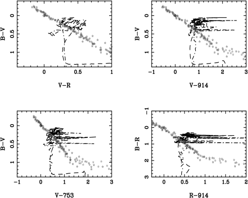
Figure 8: Simulated colors of stars (from the Pickles’ library) and active galaxies (z=0-3); dashed line: AGN template (Vanden Berk et al. 2000); dot-dashed line: starburst template (Kinney et al. 1996). The spikes in the medium-band filters are produced by strong emission lines that enter the filter.

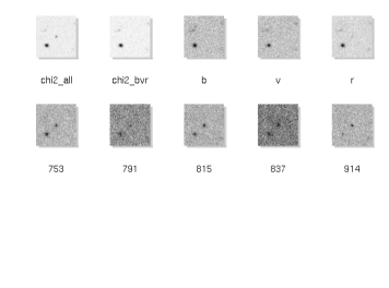
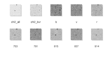
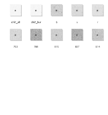
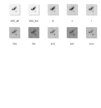
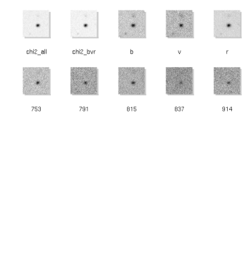
Figure 9: Examples of candidates for: nearby active galaxies (top); high-z active galaxies (middle); R-dropouts (bottom). For each source, the images are taken from the $\chi^{2}$ built from all bands, the one built from the broad-band filters only, and each filter separately. chi2_all means the $\chi^{2}$ image for all the bands while chi2_bvr means the $\chi^{2}$ image for the B,V and R bands.

6.2 Search for AGNs and high-redshift objects

We used HYPERZ to compute the colors expected for our photometric system from normal and active (starburst + active galactic nuclei) galaxies. To this aim we used as templates the composite quasar spectrum from the Sloan Digital Sky Survey (Vanden Berk et al. 2000) and the starburst templates from Kinney et al. (1996) and convolved them with the filter+CCD transmission curves. The results are displayed in Figure 8. This allowed to produce a first set of selection boxes for candidates of (i) nearby (z $<$ 2) active galaxies (B-V $\leq$ 0.2, 0.3 $\leq$ V-R $\leq$ 0.7) and (ii) high-redshift (z $\geq 2$) active galaxies (B-V $\geq$ 0.8, 0 $\leq$ V-R $\leq$ 0.7). Thanks to the $\chi^{2}$ image, built from the images in all filters, it is also easy to look for (iii) sources detected in the medium-band filters only. These may be either emission-line galaxies where a line enters a medium-band filter, medium-redshift (z $\sim$ 1) elliptical galaxies where the 4000Å break enters the R filter, or high-redshift (z $\geq 5$) galaxies where the Ly$\alpha$ break enters the R filter, Some examples from these three groups are displayed in Figure 9. Spectroscopic follow-up is being carried out, that should allow to validate and refine these criteria.

6.3 Search for white dwarfs

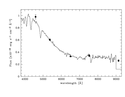
Figure 10: Spectrum of a WD candidate obtained at the ESO 3.6m telescope with EFOSC2. The fluxes obtained from aperture photometry are also reported (black dots) and are in good agreement with the spectroscopic data. The flat behaviour in the red part of the spectrum, starting near 7000 Å, suggests the presence of a cool companion.

The White Dwarf Luminosity Function (WDLF) contains crucial information on the genesis of our galaxy: age of the galactic disk and halo, IMF, stellar formation rate. Moreover the recent results of the MACHO+EROS microlensing experiments indicate that the microlensing events are mainly produced by halo objects with an average mass of $\sim$0.5 $M_{\odot}$(Alcock et al. 2000), suggesting that part of the dark matter might be formed by halo white dwarfs. The discovery of very cool WDs with $T_{\rm eff}$ $<$ 4000 K, whose statistic is almost totally unknown (less than 10 objects known up to date), is fundamental to improve our knowledge on the questions addressed.

The aim of this research is to confirm spectroscopically the nature of a few WD candidates with R magnitudes between 17.8 and 22.3, selected through their colors from the OACDF survey. For more details on the color selection see Silvotti et al. (2002). Actually the WDs which can be well separated from the MS (Main Sequence) stars are those with extreme (very high or very low) temperatures. Moreover only the hydrogen WDs move out from the MS at very low temperatures (${}^{<}_{\sim}$ 4000 K) and become bluer in V–I because of the molecular hydrogen absorption (Hansen 1998), whereas the helium WDs become more and more red as they proceed along their cooling track, without leaving the MS region.

Presently spectra of about 10 WD candidates from the OACDF, obtained at the 3.6m+EFOSC2 and NTT+EMMI ESO telescopes in March and April 2002, are under reduction. As an example, a spectrum of a White Dwarf is shown in Figure 10; a preliminary comparison between the H$\beta$ FWHM and the LTE DA models from Koester (private communication) gives an effective temperature of the order of 14000 K (considering a surface gravity $\log g$=8.0 in cgs units).

References

- [1] Alcock C., Allsman R.A., Alves D.R., et al., 2000, ApJ 542, 281
- [2] Baade D., Meisenheimer K., Iwert O., et al., 1998, The ESO Messenger, 93, 13
- [3] Bolzonella, M., Miralles, J.-M, Pelló R. 2000, AA, 363, 476
- [4] Hansen B.M.S., 1998, Nature 394, 860
- [5] Jacoby G.H., Quigley R.J., Africano J.L., 1987, PASP, 99, 672
- [6] Kinney A.L., Calzetti D., Bohlin R.C. et al. ApJ 467, p. 38, 1996.
- [7] Landolt A.U., 1992, AJ, 104, 340
- [8] Pickles A.J. 1998, PASP, 110, 863
- [9] Silvotti R., Alcalá J.M., de Martino D., Garcia Berro E., Isern J., 2002, Proc. of the 13th European Workshop on White Dwarfs, eds. D. de Martino, R. Kalytis, R. Silvotti & J.-E. Solheim, Kluwer Academic Publishers, in press
- [10] Stetson P., 2000, ”Stetson Photometric Standards”, web site: http://cadcwww.hia.nrc.ca/standards/
- [11] Szalay A., Connolly A.J. and Szokoly G.P. 1999, ApJ, 117, 68
- [12] Vanden Berk D.E., Richards G.T., Bauer A. et al. 2000, AJ, 122, 549