The X-ray Reflectors in the Nucleus of the Seyfert Galaxy NGC 1068

Abstract

Based on observations of the Seyfert nucleus in NGC 1068 with ASCA, RXTE and BeppoSAX, we report the discovery of a flare (increase in flux by a factor of $\sim$ 1.6) in the 6.7 keV Fe K line component between observations obtained four months apart, with no significant change in the other (6.21, 6.4, and 6.97 keV) Fe K$\alpha$ line components. During this time, the continuum flux decreased by $\sim$20%. The RXTE spectrum requires an Fe K absorption edge near 8.6 keV (Fe XXIII $-$ XXV). The spectral data indicate that the 2$-$10 keV continuum emission is dominated ($\sim$ 2/3 of the luminosity) by reflection from a previously unidentified region of warm, ionized gas located $\lesssim$0.2 pc from the AGN. The remaining $\sim$ 1/3 of the observed X-ray emission is reflected from optically thick, neutral gas. The coronal gas in the inner Narrow-Line Region (NLR) and/or the cold gas at the inner surface of the obscuring “torus” are possible cold reflectors. The inferred properties of the warm reflector are: size (diameter) $\lesssim$0.2 pc, gas density $n\gtrsim$ 10^5.5 cm^-3, ionization parameter $\xi\approx$ 10^3.5 erg cm s^-1, and covering fraction 0.003 (L₀/10^43.5 erg s^-1)${}^{-1}<(\Omega/4\pi)<$ 0.024 (L₀/10^43.5 erg s^-1)${}^{-1},$ where L₀ is the intrinsic 2$-$10 keV X-ray luminosity of the AGN. We suggest that the warm reflector gas is the source of the (variable) 6.7 keV Fe line emission, and the 6.97 keV Fe line emission. The 6.7 keV line flare is assumed to be due to an increase in the emissivity of the warm reflector gas from a decrease (by 20$-$30%) in L₀. The properties of the warm reflector are most consistent with an intrinsically X-ray weak AGN with L${}_{0}\approx$ 10^43.0 erg s^-1. The optical and UV emission that scatters from the warm reflector into our line of sight is required to suffer strong extinction, which can be reconciled if the line-of-sight skims the outer surface of the torus. Thermal bremsstrahlung radio emission from the warm reflector may be detectable in VLBA radio maps of the NGC 1068 nucleus.

1 Introduction

NGC 1068 is one of the original “spiral nebulae” that were noted by Seyfert (1943) to have strong, high-excitation emission lines in their nuclear optical spectra. Its lack of “broad” (FWHM $\gtrsim$ 1000 km s^-1) emission lines from a “broad-line region” (BLR), argued to be present in type 1 Seyfert nuclei, identify it as a type 2 Seyfert galaxy. However, when broad Balmer emission lines were discovered in its polarized optical nuclear spectrum by Antonucci & Miller (1985), it became clear that this galaxy contained a “hidden” broad-line region, seen only in light reflected around an intervening obscuring medium. This result, combined with results for other Seyfert galaxies, gave rise to the so-called unified model of active galactic nuclei (AGNs), which asserts that the difference between type 1 and type 2 AGNs is due to the relative orientation of an optically thick torus which surrounds the central engine and BLR (cf. Antonucci 1993 and references therein).

X-ray observations of AGNs have, for the most part, supported this unified model. For example, observations of X-ray bright type 2 Seyfert galaxies with the HEAO-1 satellite (Mushotzky 1982) showed that their X-ray spectra were well represented by a power-law with photon index $\Gamma\approx$ 1.8 (characteristic of type 1 Seyferts), with additional absorption with column densities N${}_{H}\gtrsim$ 10²² atoms cm^-2. The absorption column in type 2 Seyfert galaxies, typically $\sim$10²³$-$10²⁴ cm^-2, is assumed to be due to the blocking torus (e.g., Mulchaey, Mushotzky & Weaver 1992).

Higher quality data now show that Seyfert X-ray spectra are more complex than a simple absorbed power-law. In many type 2 objects, a ‘soft excess’ (soft X-ray emission in excess of that expected from a simple absorbed power-law) is common below $\sim$2 keV (e.g. Turner & Pounds 1989). Above $\sim$10 keV, the power-law slope generally flattens (e.g., Nandra & Pounds 1994) due to Compton scattering of nuclear light reflected from the accretion disk (ergo, the “reflection component”). Soft X-ray absorption lines (e.g., due to O, Ne, Mg, Si, Fe) from an ionized medium are also present (cf. Reynolds & Fabian 1995). And finally, between 6 and 7 keV, strong Fe K$\alpha$ fluorescence lines are present, and are thought to originate from the accretion disk, or, in some cases, from the inner edge of the torus.

The central region of NGC 1068 contains a starburst (e.g., Wilson et al. 1992), which produces a large fraction of the X-ray emission below $\sim$4 keV (e.g., Levenson et al. 2001). At higher energies, the AGN dominates the spectrum. The X-ray spectrum of the AGN is particularly interesting, in that it has an Fe K$\alpha$ line with a very large equivalent-width (EW), first discovered with GINGA by Koyama et al. (1989), who modelled the spectrum with a relatively flat ($\Gamma\sim$ 1.5) power-law with little or no absorption, plus a single Gaussian line centered at 6.55 keV with EW of 1.3 keV. Compare this with typical EWs for type 1 Seyferts, which are $\lesssim$500 eV (e.g., Nandra et al. 1997). Such a large EW was predicted by the X-ray scattering model of Krolik & Kallman (1987), although the measured EW in NGC 1068 is larger than predicted. It was suggested that the observed (reflected) X-ray continuum flux is much smaller than that illuminating the fluorescing material, resulting in a larger EW than for Seyfert 1 galaxies. Higher-resolution X-ray spectral data obtained with BBXRT showed three separate narrow Fe K$\alpha$ components with a net EW of 2.7 keV (Marshall et al. 1993). Marshall et al. suggested that the multiple Fe K features arose from two components of the nuclear gas, a hot and a warm component. A revised model of the X-ray continuum for NGC 1068 was later put forward by Smith, Done & Pounds (1993), who found that although a reflection component was not required by the GINGA data, if it were included, it would change the inferred intrinsic power-law slope to $\Gamma\sim$ 1.9, more typical of Seyfert 1 X-ray spectra. More recent ASCA data have confirmed the three separate line components, this time with a total EW of 3.2 keV (Ueno et al. 1994). Using the same ASCA data, Iwasawa et al. (1997) proposed the existence of a fourth Fe K component $-$ a weak red wing of the 6.4 keV fluorescence line, possibly due to Compton scattering in optically thick, cold matter (Matt et al. 1996). Hard ($\gtrsim$10 keV) X-ray emission detected by BeppoSAX (Matt et a. 1997) is consistent with reflection from a mixture of neutral and ionized gas, with an intrinsic power-law slope of $\Gamma\sim$ 1.7.

In this paper, we further investigate the nature of the X-ray emission due to the AGN by analyzing the broad-band (E $\approx$ 4$-$200 keV) X-ray spectrum using all of the available data from the ASCA, RXTE and BeppoSAX missions. We focus here only on the X-ray spectrum above 4 keV to avoid the nuclear starburst. The hard ($\gtrsim$ 10 keV) X-ray spectral coverage provided by the RXTE and BeppoSAX Phoswich Detector System (PDS) data is vital for placing constraints on continuum models. After the continuum is well modelled with the best data available, we can then accurately model the Fe K$\alpha$ complex. Such is the goal of the current paper. In section 2, we describe the data used for our analyses and describe details of the data reduction. Section 3 contains the primary observational results from our analyses and section 4 contains a discussion of the implied physical constraints on the geometry of the nucleus of NGC 1068 and the origin of the X-ray emission. Throughout this paper, we assume a distance of 14.67 Mpc (H${}_{0}=$ 75 km s^-1 Mpc^-1) to NGC 1068.

Figure 1: Timeline of relevant X-ray spectral observations of NGC 1068. ASCA observations are shown as filled triangles, RXTE observations are shown as filled rectangles, and BeppoSAX observations are shown as open rectangles. Note that the RXTE observation is simultaneous with the second ASCA observation (ASCA2).

2 Observations and Data

We restrict photon energies to be $>$ 4 keV, to avoid any starburst emission. A timeline of the relevant spectral observations is shown graphically in Figure 1, showing the following four epochs: (epoch 0) ASCA1, (1) ASCA2/RXTE, (2) SAX1 and (3) SAX2. In this paper, we concentrate mainly on the data from epochs 1 and 2, thus our odd numbering scheme. Additional information about the observations are listed in Table 1.

2.1 ASCA Observations

Data from the two archival ASCA observations were retrieved from the US archives at the NASA/GSFC High Energy Astrophysics Science Archive Research Center (HEASARC). Both the Solid-state Imaging Spectrometers (SIS0 and SIS1), and the Gas Imaging Spectrometers (GIS2 and GIS3) were used in our analyses. The data were screened as follows. SIS data data were obtained in bright mode. Observing times with high background were removed, based on the recommended criteria in the ASCA data analysis guide. Hot and flickering pixels were discarded, as were data when the satellite passes through the South Atlantic Anomaly (SAA), when its elevation above Earth’s limb is $<5^{\circ}$ (night) or $<20^{\circ}$ (day), when the geomagnetic cutoff rigidity is $<6$ GeV c^-1, and when the time is $<32$ s after a day/night transition, or $<32$ s after an SAA passage. Background counts were accumulated from source-free regions near the target and then subtracted. The ASCA spectra were grouped to have $\geq 30$ photons in each energy bin.

2.2 RXTE Observations

The RXTE Proportional Counter Array (PCA) data were taken simultaneously with the second ASCA observation (ASCA2). The PCA consists of five Proportional Counter Units (PCUs), three of which were reliable during the observation. PCA Standard Mode 2 data were reduced with the REX (v0.2) script from FTOOLS (v5.0.1), using the default selection criteria, as follows. Data were extracted only from layer 1, and only from PCUs 0, 1 and 2; for Earth elevation angle $>$10^∘, pointing offset $<$0.02^∘, “electron contamination” $<$0.1, and times $>$30 min after the peak of the last SAA passage. The background was estimated using PCABACKEST (v2.1e), using the L7-240 background model, recommended for faint sources by the NASA/GSFC RXTE Guest Observing Facility. The L7-240 model is composed of two components: ‘L7’ and ‘240.’ The ‘L7’ component estimates the internal detector background derived from a combination of 7 rates in pairs of adjacent signal anodes, read directly from the Standard 2 data files. The ‘240’ component estimates the effect of particles present in the detectors after an SAA passage, assuming a decaying exponential with half-life 240 s. The response matrix was generated using the FTOOLS task PCARMF (v3.7).

2.3 BeppoSAX Observations

Both sets of BeppoSAX data were retrieved from the archives at the BeppoSAX Science Data Center (SDC) in Rome. Only data from the Medium-Energy Concentrator Spectrometers (MECS) and the PDS instruments were used. Raw data were processed by the SDC’s Supervised Standard Science Analysis (Rev. 0 for the SAX1 data and Rev. 1.1 for the SAX2 data). We used BeppoSAX SDC calibration and background data released in November 1998.

The first observation (SAX1) occurred before MECS instrument no. 1 failed (i.e., before May 7, 1997), so events from all three MECS were available. SAX1 MECS spectra were extracted using circular regions of radius 4′ and then combined into one spectrum by routine pipeline processing by the BeppoSAX SDC. The combined spectrum was then grouped so that it had a minimum of 20 counts per spectral bin. Background data were taken from a 4′ source region from SDC background events files. The spectral data from the PDS instrument were not modified from their original condition after being processed by the SDC. The PDS data were grouped according to the default grouping file (provided by the SDC). PDS data processed by the pipeline processing of the BeppoSAX SDC are already background-subtracted.

Only two MECS instruments were available during the second SAX observation (SAX2), since MECS no. 1 had failed by that time. The SAX2 MECS and PDS data were processed in a similar manner to the SAX1 data, although source and background counts were extracted using circular regions of 3′.

2.4 Notes on Spectral Data

Our first goal is to constrain X-ray continuum models of the AGN, so we concentrate on the spectral data with the highest signal-to-noise ratio and the best broad-band (from $\sim$4 to greater than 10 keV) coverage. Compton reflection is expected to contribute significantly to the continuum shape at energies $\gtrsim$ 10 keV, so the ASCA spectra ($\lesssim$10 keV) alone do not constrain this component well. However, ASCA data are needed to accurately model the Fe K$\alpha$ complex. The RXTE data spectral response (up to $\sim$ 40 keV) is ideally suited to model the Compton reflection component, while the BeppoSAX MECS instrument offers good coverage of the Fe K region and the $\sim$4$-$10 keV continuum. The BeppoSAX PDS data have low resolving power, but are useful in constraining the high-energy X-ray continuum (up to $\sim$100 keV). Since the SAX1 data have much longer exposure times than the SAX2 data (Table 1), and were taken nearer to the time of the epoch 1 data, we use them for modelling the broad-band X-ray spectrum.

We therefore initially used the simultaneous ASCA2 and RXTE data (epoch 1), and the SAX1 (epoch 2) data, taken four months later. XSPEC v11.1.0 is used for all spectral fits. All errors are quoted at the 90% uncertainty level for one interesting parameter ($\Delta\chi^{2}=$ 2.7).

3 Spectral Fitting Results

3.1 The 4$-$100 keV X-ray Spectrum

Because the spectrum of NGC 1068 is complex, assumptions about the spectral structure of the Fe K region may affect our continuum model. In this section, we investigate potential continuum components using four different simple continuum models, together with two Fe K line emission models. For the line models, we use four Gaussian components, first an empirical model which provides a good fit, and, second, a “narrow-line” model with fixed central energies. The continuum models are: (1) an absorbed power-law, (2) reflection from optically thin ionized gas (power-law plus an Fe K edge), (3) reflection from optically thick neutral gas (XSPEC constant-density model pexrav; Magdziarz & Zdziarski 1995), and (4) reflection from optically thick ionized gas (pexriv). Galactic absorption was included with N_H fixed at 3.53 $\times$ 10²⁰ cm^-2 (Dickey & Lockman 1990). Relative normalization constants for each detector were allowed to vary, but were constrained to be within ranges determined from cross-calibration studies (see section 3.1.3).

3.1.1 High-energy Continuum

In order to test for variability in the hard continuum between epochs, we fit the RXTE, SAX1 PDS, and SAX2 PDS spectra individually with an absorbed power law model. The 12$-$40 keV flux and the spectral indices are consistent with no variation between each of the three observations. Therefore, fitting the epoch 2 SAX1 PDS data together with the epoch 1 ASCA and RXTE data is justified.

3.1.2 Empirical Model for the Fe K complex

For the purposes of finding the best continuum model, we first take an empirical approach to modelling the Fe K$\alpha$ line complex, using only the epoch 1 data (ASCA2 and RXTE). Following Iwasawa et al. (1997), we model the Fe K line complex with four Gaussian components, but allow the line energies and line widths to vary. After trying the continuum models, we found that the best fit model was for an optically thick ionized reflection continuum model ($\xi\approx$ 2000 erg cm s^-1) with Gaussian central energies (and line widths $\sigma$) at 6.21 (0.01), 6.38 (0.05), 6.59 (0.007), and 6.84 (0.09) keV. We attach no physical significance to these energies and line widths, and note only that they fit the spectral data well.

We then fixed the central energies, line widths, and line fluxes to the values from this fit and proceeded to fit the epoch 1 and 2 data together. The ionized reflection models are again significantly preferred over the other two models ($\chi^{2}$/dof $=$ 486/419 and 498/419, for the optically thick and optically “thin” models, compared to 532/420 and 536/420, for the absorbed power-law and neutral reflection models, respectively). Such a large difference in $\chi^{2}$ suggests that the dominant component of the continuum emission is indeed reflection from an ionized plasma. Both the optically thick and optically thin ionized reflection models (the best fit models) require an edge from ionized Fe at E $\approx$ 8.6 keV (Fe XXIII $-$ XXV). The best-fit Fe K edge depth $\tau_{edg}$ is $\sim$0.5 for the “optically thin” model, which is not really in the optically thin or thick range. Since there is no available model for reflection from ionized gas with $\tau\approx$ 0.5 (see footnote), in the remainder of the paper, we show results from both our PEXRIV (optically thick) and power-law-plus-edge (optically thin) models.

Figure 2: Ratio plot (data to model) of the Fe K$\alpha$ spectral region for the absorbed power-law model. Data from both epoch 1 and epoch 2 (ASCA2, RXTE and SAX1) were used in this joint fit (see section 3.1.2). At left, we show the ratio of the epoch 1 ASCA and epoch 2 MECS data to the power-law model without Fe lines, while at right we show the ratio of the data to the power-law model with the four-Gaussian model described in section 3.1.2. The top four panels at right show no significant residuals, while the epoch 2 MECS ratio plot at bottom right shows excess emission centered at $\sim$6.7 keV.

The reduced $\chi^{2}$ values for the ionized reflection models ($\chi_{\nu}\approx$ 1.2) further suggest that some features are still not well modelled. Indeed, the epoch 2 MECS spectrum shows excess emission centered near 6.7 keV. In Figure 2, we show the ratio of the data to the absorbed power-law model for energies near the Fe K complex. While the epoch 1 ASCA2 detectors (top four panels) show no consistent residual line emission, residuals are clearly evident at $\sim$6.7 keV in the epoch 2 MECS spectrum (bottom panel). The result is not an artifact of the continuum model, since ratio plots using the other continuum models show the same result. This demonstrates variability in the Fe K$\alpha$ line complex between epochs 1 and 2 (discussed further in section 3.2). For this reason, hereafter we omit the SAX1 MECS spectrum in the fit, when fitting for the purpose of determining the broad-band continuum shape.

Now, using only the SAX1 PDS data with the ASCA2 and RXTE data (and cross-calibration constant ranges described in section 3.1.3), the fits are much better (see Table 2). For example, $\chi_{\nu}^{2}=$ 1.0 for the optically thick ionized reflection model, compared to $\chi_{\nu}^{2}=$ 1.3, when the SAX1 MECS is included. The absorbed power-law model and neutral reflection models are still not acceptable fits ($\chi^{2}$/dof = 376/322 and 401/322, respectively). The “optically-thin” ionized reflection model with an edge at $\sim$8.6 keV is also a good fit, with $\chi_{\nu}\approx$ 1.07. These results suggest that much of the nuclear X-ray emission is reflected into our line of sight by highly ionized gas with $log~{}(\xi/$ erg cm s${}^{-1})\sim$ 3. We cannot, however, discriminate between an optically thick or thin ionized reflector. The Compton reflection component provided by the optically thick model PEXRIV does give a better fit than the optically-thin reflection model ($\Delta\chi^{2}=$ 31). This suggests that at least one optically thick reflector (ionized or neutral; see also Matt et al. 1997) is present.

3.1.3 Cross-Calibration of the Instruments

Relative flux normalization constants between the various ASCA, XTE and SAX instruments have been estimated by Yaqoob et al. (2000) and Fiore et al. (2001). The results are that all ASCA instruments and the SAX MECS give the same flux values within 3%. The XTE PCAs give a 20% higher flux value, assuming that the are no effects due to their different aperture sizes. Compared with MECS, the SAX PDS gives a 15% low flux value, again assuming no aperture effects.

For the rest of the fits in this paper (the “narrow-line” fits), we restricted the calibration constants of the instruments to be within our best-estimated ranges. This is necessary to insure that any variability we find is not due to calibration differences. We first fixed the calibration of the ASCA GIS2 instrument to 1.0. All relative calibration constants of the other instruments are quoted with respect to GIS2. We allowed the calibration constants for all other ASCA instruments and the MECS to vary within a 6% uncertainty range (0.94$-$1.06). The larger aperture of the XTE PCA allows more flux from the rest of the NGC 1068 galaxy, so we determined the “best” PCA normalization constant from the empirical four-Gaussian fit to only the epoch 1 data, using our best-fit continuum model, the optically-thick ionized reflection model. The resulting range was 1.34$\pm$6%, which is consistent with Yaqoob et al.’s value, given the larger aperture of the PCA. The “best” PDS normalization constant was determined from fitting the four-Gaussian empirical models to both the epoch 1 and 2 data. All continuum models gave the same result, 0.81, thus we used a range of 0.81$\pm$6% for the PDS. This range is also consistent with the estimated value from the SAX calibration team.

3.1.4 Narrow-line Fixed-Energy Model for the Fe K complex

We next model the Fe K$\alpha$ line complex with three narrow ($\sigma=$ 0) Gaussian lines and fix the central energies of the lines to those of the expected strong atomic transitions or other observed features: 6.40 keV (‘neutral’ Fe K$\alpha_{1}$ and K$\alpha_{2}$ transitions), 6.70 keV (He-like Fe XXV), and 6.97 keV (H-like Fe XXVI). Adding a line at 6.6 keV (to represent the blend of Fe XXV and XXIV lines expected in a hot plasma, e.g., Beiersdorfer et al. 1993; Feldman, Doschek & Kreplin 1980) does not improve the fit and so we omit that feature. However, the ‘Compton shoulder’ feature at $\approx$ 6.2 keV (Iwasawa et al. 1997) is significant, so we include an additional line at 6.21 keV and fix its width $\sigma$ to 150 eV. Line fluxes were allowed to vary. This narrow-line model is consistent with the Chandra HETG spectra of the NGC 1068 nucleus published by Ogle et al. (2001), who find that the Fe line complex is fit very well with unresolved Fe lines at these energies, with no evidence for a broad Fe line component (P. Ogle, priv. comm.).

Using this narrow-line model, the ionized reflection continuum models are again clearly preferred over both the absorbed power-law and neutral reflection models, as they were for the empirical Fe-line model. The line fluxes are not significantly different for the four models (see Table 3), indicating that the line parameters are not strongly correlated with the choice of continuum model.

In summary, both the empirical and narrow-line methods of modelling the Fe K features imply that the continuum flux from NGC 1068 includes a reflected component from highly ionized gas. For both optically thick and optically “thin” ionized reflection models, the Fe absorption edge energy is $\sim$8.6 keV, implying that the ionization parameter $\xi$ of the warm reflector has a value $log\xi\sim$ 3. Implications of these results are discussed in section 4.

3.2 A Variable Fe K line

As mentioned in section 3.1.2, there is excess line emission in the MECS centered $\sim$ 6.7 keV (Figure 2), implying an increase in the epoch-2 6.7 keV line flux, compared to epoch 1. Here, we investigate this variability further by fitting the narrow-line models discussed above (section 3.1.4) to all of the epoch 1 and epoch 2 data simultaneously. We perform fits using all four continuum models, for completeness.

First, we froze the the continuum model parameters for both epoch 1 and 2 data to those listed in Table 2 (the ‘epoch 1’ values), while the four epoch 2 Fe K line fluxes were allowed to vary. Initially, we did not allow the continuum (i.e. power-law normalization) to vary between epochs. However, simply allowing the power-law normalization to vary improved the fit enormously ($\Delta\chi^{2}=$ 70$-$80) and consistently showed a decrease in the continuum flux by 20% (uncertainty of 5$-$10%), independent of the choice of continuum model. We discuss the continuum variability further in sections 3.3 and 4. The resulting line fluxes for the variable-norm case for both epochs are listed in Table 3 and are shown graphically in Figure 3. Although we do not favor the constant-norm case, we also list fluxes for it in Table 3. Although the ionized reflection continuum models (2 and 4) are clearly preferred over the other two continuum models, as a precaution, we also performed the same test for the absorbed power-law and neutral reflection continuum models. The 6.7 keV line flux is consistently a factor of $\sim$1.6 higher in epoch 2, while the 6.4 keV line flux is statistically consistent with no variation. The larger epoch 2 value for the 6.7 keV line flux is consistent with measurements from recent Chandra HETG data (P. Ogle, priv. comm.).

Figure 3: Line fluxes (Table 3) for the four Gaussian Fe K “narrow-line” components for epochs 1 and 2, assuming the continuum shape did not vary between epochs, but allowing the power-law norm (continuum flux) to vary. The best-fit ionized reflection models (models 2 and 4) show the main result, which is that the 6.7 keV line component increased in 4 months. For completeness, the other two models are shown. See Table 2 for descriptions of continuum models. Error bars are 90% confidence ($\Delta\chi^{2}=2.7$).

Figure 4: Line fluxes (Table 3) for the four Gaussian Fe K “narrow-line” components for epochs 1 and 2, when the continuum slope $\Gamma$ is allowed to vary between epochs. Again, the best-fit models (2 and 4) show that the 6.7 keV line increased between epochs.

In order to ensure that the increase in the 6.7 keV line flux was not due to a change in the continuum shape, we also allowed various continuum model parameters to vary between epochs (see Table 3 and Figure 4). The main result is that the flux in the 6.7 keV component shows an increase regardless of the continuum shape. We should note that for several cases using the the neutral reflection model, while the 6.7 keV line flux does show an increase, it is not at the 90% confidence level. However, we also note that the neutral reflection model is a very poor fit to the broad-band spectrum. The ratio in the line flux (epoch 2/epoch 1) ranges from 1.53 to 1.75 for the best-fit ionized reflection models (models 2 and 4). Thus, we can say with confidence that the structure of the Fe K line complex has varied in the four months between the two epochs, and, in particular the 6.7 keV line flux has increased by a factor of 1.53$-$1.75. For the case when the continuum spectral shape did not change, but the continuum flux did, the increase factor in the 6.7 keV line flux is 1.6$-$1.7, for the best-fit ionized reflection models.

We have also attempted to model the Fe K variability in other ways. If the central line energy of the “6.7 keV” line is allowed to vary from 6.70 keV while fitting, it does not deviate from 6.70 keV. If we further allow the line width $\sigma$ to vary, it increases to 0.12 keV. Even in this case, the 6.7 keV line flux variability is still comparable to that for the narrow-line Fe model, while the other line fluxes are consistent with those in Table 3. Thus, even if the line width has increased, the line flux has increased as well.

We also fit the Fe K complex with 6.4 and 6.7 keV lines using a relativistic disk model (XSPEC model diskline) to see if the variability could be modelled in terms of physical variations in the accretion disk (e.g., the inner radius of the accretion disk). We first tried replacing only the 6.7 keV Gaussian line with a disk line, and then tried replacing both the 6.4 keV line and the 6.7 keV line with a disk line. However, for both face-on (i $\sim$ 30^∘) and edge-on (i $\sim$ 70^∘) disks, the disk model is a poor fit, regardless of the central energy. We obtain $\chi^{2}>$ 500 for a combined fit with epoch 1 and 2 data with an ionized reflection continuum model, compared with $\chi^{2}\sim$ 400$-$420 for pure Gaussian line fits in Table 3. The fit is poor regardless of what central energy is used for the line and whether the continuum is allowed to vary between epochs. Therefore, we conclude that either a relativistic disk line of this variety is not present, or, if it is present, the Fe K complex has too many components to be able to model it directly with current data. The recent Chandra HETG grating spectrum of the NGC 1068 nucleus also shows no evidence for a broad Fe line component (Ogle et al. 2001), which supports our conclusion that there is no dominant broad Fe line component present in our data.

3.3 Long-term Variability of the continuum

Figure 5: Continuum flux measurements for four epochs of NGC 1068 X-ray data: (epoch 0) ASCA1, (1) ASCA2, (2) SAX1 and (3) SAX2. The ionized reflection continuum model was assumed, but other models give similar results. The filled rectangles are the 4$-$5 keV flux (no Fe K emission) in units of 10^-13 erg s^-1 cm^-2, and the open rectangles are the 4$-$10 keV flux (including the Fe K emission) in units of 10^-12 erg s^-1 cm^-2. The 4$-$10 keV flux points are offset by $+$0.1 yr for clarity. The plotted uncertainties are $\pm$20%.

We also checked for variability of the continuum flux between all four epochs of data. In Figure 5, we show the 4$-$10 keV flux (including the Fe K emission; open rectangles) and the 4$-$5 keV flux (solid rectangles) from the ASCA GIS2 or SAX MECS instruments. Between the two epochs for which the 6.7 keV component varied (epochs 1 and 2), the continuum flux decreased by 18%, consistent with the 20% value obtained in section 3.2. The 20% error bars in the plot correspond with typical 90% confidence ranges of the power-law norm (“N” in Table 3) when several interesting parameters were allowed to vary. We conclude that the continuum flux did not vary more than 20% over the entire timespan (from 1993.5 to 1998), assuming the continuum shape is allowed to vary. If the continuum shape did not vary between epochs 1 and 2, the flux decreased by $\approx$20%, with a subsequent rise in flux between epochs 2 and 3.

It is worth noting that the $\chi^{2}$ values are consistently lowest, or very nearly lowest, for the fits in which only the power-law norm and the Fe K line fluxes vary between epochs 1 and 2 (see Table 3). Thus, this simple model suggests both an increase in the 6.7 keV line flux and a decrease in the continuum flux.

3.4 Summary of Results

Here we summarize the results from this section. When the epoch 1 spectral data are fit with Gaussians to model the Fe K lines, plus the following continuum models, (1) an absorbed power-law, (2) an “optically-thin” ionized reflection model (power-law plus edge), (3) an optically-thick neutral reflection model (PEXRAV), or (4) an optically-thick ionized reflection model (PEXRIV), the best fit models are (2) and (4). Both of these models fit the edge observed in the RXTE data at $\approx$8.6 keV. This edge energy implies an ionization parameter $\xi\sim$ 10³ erg cm s^-1. Model (4) gives a better fit than model (2), suggesting that Compton reflection is needed (from optically-thick ionized gas), or, from an additional component of optically thick neutral gas. When the epoch 2 data and the epoch 1 data (taken 4 months apart) are jointly fit, the continuum is noted to decrease by $\approx$20%, while the 6.7 keV Fe K line component is observed to increase by a factor of $\approx$1.6.

4 Discussion

In the subsections below, we discuss the location and physical properties of the X-ray reflection regions in the nucleus of NGC 1068. We also discuss the implications for the reflection of light at other wavelengths.

4.1 The Intrinsic X-ray Luminosity of the AGN

The common AGN paradigm predicts that, for type 2 active galaxies, direct emission from the AGN is partially or fully blocked by an optically and geometrically thick torus (cf. Antonucci 1993), so the intrinsic X-ray luminosity L₀ cannot be measured directly. Even so, we can estimate L₀ using the correlation between the 2$-$10 keV X-ray luminosity and the [O III] $\lambda$5007 optical line luminosity for Seyfert nuclei (e.g., Mulchaey et al. 1994): log([O III]/L_X) $=$ $-$1.89$\pm$0.25 for type 1 Seyferts and log([O III]/L_X) $=$ $-$1.76$\pm$0.38 for type 2 Seyferts. We use the correlation for type 1 Seyferts here, since some of the X-ray emission in type 2 Seyferts is absorbed. Using the nuclear [O III] flux from Whittle (1992), we estimate the intrinsic 2$-$10 keV X-ray luminosity of the AGN to be $L_{0}=$ 10^43.5 erg s^-1 (with an uncertainty of $\sim$0.25 in the log). As a comparison, Pier et al. (1994) estimate the intrinsic bolometric luminosity of NGC 1068 to be 3.8 $\times$ 10⁴⁴ erg s^-1 (for a relative reflection fraction f${}_{refl}=$0.01). Assuming L_X(2$-$10 keV)/L_Bol $\sim$ 0.1 for AGN (e.g., Elvis et al. 1994), their estimate of $L_{0}$ is consistent with that predicted from the [O III]/L_X relationship.

4.2 The 6.7 keV Line Emitting Region

4.2.1 Size

The variability of the 6.7 keV line luminosity in the four months between epochs 1 and 2 suggests that the maximum size of the line-emitting region is approximately the light travel time of 4 light months (0.1 pc). However, since the variation is only a factor of $\approx$1.6, the size $l$ (treated as a diameter) could be a factor of several larger than the light travel time. Hereafter, we write the size $l$ in terms of our fiducial value 0.1 pc ($l=l_{0.1}$ 0.1 pc) and note that $l_{0.1}\lesssim$ 2.

4.2.2 Density

A lower limit to the density can be estimated from the line flux $F$, since

$$F={{\eta\int n^{2}dV}\over{4\pi D^{2}}}$$

and the volume $V$ is limited by the size $l$. The combined emissivity $\eta$ for the three 6.7 keV lines (at 6.641, 6.669 and 6.683 keV) is plotted in Figure 6, along with the emissivity for the 6.97 keV line.

Figure 6: Emissivities $\eta$ of the 6.7 and 6.97 keV lines, as a function of the logarithm of the ionization parameter $\xi=L_{0}/nR^{2}$. These values of $\eta$ were calculated using XSTAR v1.45, assuming $T=$ 10⁷ K.

For simplicity, we take $\eta=\eta_{-16}$ $\times$ (1.0 $\times$ 10^-16 photons cm³ s^-1), where $\eta_{-16}$ is of order 1. We next write $\int n^{2}dV=\bar{n}^{2}\phi~{}l_{0.1}^{3}$ $\times$ (1.4 $\times$ 10⁵² cm^-3), where the filling factor $\phi$ (for a spherical volume) is less than 1.0, and the cloud diameter $l_{0.1}\lesssim$ 2. The line flux $F=f_{6.7}$ $\times$ (5.0 $\times$ 10^-5 photons cm^-2 s^-1), where $f_{6.7}$ is also of order unity ($f_{6.7}=$ 0.7 and 1.1$-$1.2 for model 2 for epochs 1 and 2, respectively). For a distance $D=h_{75}^{-1}$ $\times$ (14.67 Mpc), we can then write

$$\bar{n}_{6.7}\approx 10^{6}\left({f_{6.7}\over\eta_{-16}\phi l_{0.1}^{3}}\right)^{1/2}h_{75}^{-1}\;{\rm cm^{-3}}$$

Since $\eta_{-16}<$ 1.8, $\bar{n}_{6.7}\gtrsim$ 10^5.5 cm^-3 to order of a few, since $\phi<$ 1 and $l_{0.1}<$ 2. Note that for R $\lesssim$ 0.1 pc, the ionization time scale for Fe XXV, $t_{ion}\sim 4\pi R^{2}E_{6.7~{}keV}/L_{0}\sigma_{ion}\approx$ 2 hr, for $L_{0}=$ 10^43.5 erg s^-1 and $\sigma_{ion}(FeXXV)\approx$ 5 $\times$ 10^-20 cm² (e.g., Verner et al. 1996), so photoionization equilibrium is established much faster than the variability time scale of 4 months.

4.3 6.97 keV Line Emitting Region

The 6.97 keV line is only strong for $\xi\gtrsim$ 10^3.0 erg cm s^-1 (see Figure 6), where $\eta\approx$ 2.5 $\times$ 10^-17 photons cm³ s^-1. The density can also be estimated from the 6.97 keV line flux $F=({\eta\int n^{2}dV})/({4\pi D^{2}})\approx$ 1.0 $\times$ 10^-5 photons cm^-2 s^-1, which requires $\bar{n}_{6.97}\gtrsim 10^{5.9}/(\phi l_{0.1}^{3})^{1/2}h_{75}\;{\rm cm^{-3}},$ very similar to the density estimate of the 6.7 keV line emitting region.

4.4 The 6.4 keV Line Emitting Region

The line flux of the 6.4 keV line component is generally 10$-$20% larger in epoch 2. However, the uncertainties in the line flux are larger than this, so a constant value for both epochs is consistent with the data, regardless of continuum model (see Table 3 and Figures 3 and 4). The large equivalent width of the 6.4 keV component (EW $\sim$ 1 keV) is almost certainly due to blockage of the direct X-ray continuum from the AGN, which would exclude the possibility that the line originates from the accretion disk. Thus, the line emission likely originates from cold gas further out (e.g., narrow-line clouds, or the inner edge of the torus; Krolik, Madau, & Zycki 1994, Ghisellini, Haardt, & Matt 1994).

4.5 Ionization Parameter and Size of the 6.7 keV and 6.97 keV Line Emitting Region

From the emissivity plot in Figure 6, we can see that the 6.7 keV line emissivity is maximized for $\xi\sim 10^{3}$ erg cm s^-1, while the emissivity of the 6.97 keV line rises with $\xi$ until it reaches a flat maximum for log $\xi\gtrsim$ 3.5. If only a single region provides the line emission, then the observed line ratio can be used to infer the value of $\xi$ in the emission region from the predicted ratio of the two lines’ emissivities. Using Figure 7, we find that the typical observed ratio $1.7\leq F_{6.7}/F_{6.97}\leq 5.6$ (Table 3, variable power-law norm case) translates into 3.45 $\leq$ log $\xi$ $\leq$ 3.75.

Figure 7: Expected line flux ratio F(6.7 keV)/F(6.97 keV), assuming both lines originate from the same gas, as a function of the logarithm of the ionization parameter $\xi=L_{0}/nR^{2}$.

Because the emissivity of the 6.7 keV line decreases with increasing $\xi$ in this range, whereas the emissivity of the 6.97 keV line is roughly constant, we would predict on the basis of this inference that decreases in continuum luminosity (for fixed density) would lead to a rise in the 6.7 keV luminosity, but little change in the 6.97 keV line. This is just what is observed. Almost independent of the different models used for line-fits (as shown in Table 3), $F_{6.7}$ increased by 60$-$70% from epoch 1 to epoch 2 while $F_{6.97}$ is consistent with being constant. The only model showing a change in $F_{6.97}$ is the constant-flux, constant-continuum shape model, which is a poor fit to the broad-band spectral data.

Quantitatively, the observed increase in $F_{6.7}$ between these two epochs demands a decrease in $\xi$ (for this single-region model) of $\approx$ 30% (Figures 6 and 7). Such a decrease is consistent with the change in line ratio, the change in the absolute line fluxes, and the estimated 20% drop in the continuum flux (section 3.3).

Given this confirmation of our estimate for $\xi$, we can estimate the distance from the nucleus to the ionized-Fe emission line region from R $=$ (L/n$\xi$)${}^{{{1}\over{2}}}$. Using the the emission measure estimate to write the density in terms of the size of the emitting region, we have

$${{R}\over{l}}\approx 0.3\left({L_{0}\over 10^{43.5}}\right)^{{{1}\over{2}}}\left({\xi\over 10^{3.5}}\right)^{-{{1}\over{2}}}\phi^{{{1}\over{4}}}l_{0.1}^{-{{1}\over{4}}}.$$

Since $R/l$ depends very weakly on $\phi$ and $l_{0.1}$, we conclude that $R\sim l$. In other words, the ionized Fe line-emitting gas resides in a more-or-less volume-filling region very close to the nucleus. In summary, we estimate the following values for the physical parameters of the 6.7 keV and 6.97 keV line emitting region: $l\lesssim$ 0.2 pc, $n\gtrsim$ 10^5.5 cm^-3, $log~{}\xi\approx$ 3.45$-$3.75, and $R\sim l$ (Table 4).

4.6 The Continuum Reflection Zones

As mentioned previously, the observed total 2$-$10 keV X-ray luminosity $L_{obs}$ is much smaller than the estimated intrinsic X-ray luminosity. For example, when the data are fit with both a pure cold (neutral) reflector component (XSPEC model pexrav) and ionized reflection models (models 2 or 4), $L_{obs}$(2$-$10 keV) $\approx$ 1.3 $\times$ 10⁴¹ erg s^-1 (model 2; 1.4 $\times$ 10⁴¹ erg s^-1 for model 4). This corresponds to a maximum X-ray reflection fraction $f_{refl}=$ 0.004 (L₀/10^43.5)^-1.

As Pier et al. (1994) note, estimates of the reflected fraction for optical light range from 0.001 to 0.05. Miller, Goodrich & Mathews (1991) estimate a value of 0.015 from measurements of the broad H$\beta$ emission reflected from the NE knot. Unless L${}_{0}\lesssim$ 10^43.0 erg s^-1, it is quite clear that the X-ray reflection fraction is, in general, smaller than the Miller et al. value. In particular, from the joint (neutral$+$ionized reflection) fit, the neutral X-ray reflection component $L_{N}\approx$ 3.9 $\times$ 10⁴⁰ erg s^-1 (model 2; 5.4 $\times$ 10⁴⁰ erg s^-1 for model 4) corresponds to a reflected fraction for the neutral reflector of $f_{N}=$ 0.001 (L₀/10^43.5)^-1, and the ionized reflection component $L_{I}\approx$ 10.0 $\times$ 10⁴⁰ erg s^-1 (model 2; 7.3 $\times$ 10⁴⁰ erg s^-1 for model 4), corresponds to $f_{I}=$ 0.003 (L₀/10^43.5)^-1.

4.6.1 The Ionized Reflector

Since the 6.7/6.97 keV line emitting region is ionized to $\log\xi\sim 3.5$, and this is close to the $\xi$ already estimated for the warm reflection region (Table 2), we suppose that the ionized Fe lines originate from the warm reflection region. The luminosity reflected by that region is $L_{W}=(\Omega/4\pi)_{W}(1-e^{-\tau_{W}})L_{0}$, where the total scattering depth is $\tau_{W}$. Depending on details of the velocity and ionization structure of the region, resonance line scattering could make $\tau_{W}$ averaged over the 2 – 10 keV band as much as a few times greater than the Thomson depth $\tau_{Th}=nl\sigma_{Th}=0.2l_{0.1}^{-1/2}$ (section 4.2; Krolik & Kriss 1995; see also Kinkhabwala et al. 2002). We may then turn around this last equation to estimate the allowed range for $(\Omega/4\pi)_{W}$, where the limits correspond to $\tau_{W}=$ 0.14 and $\tau_{W}=\infty$:

$$0.003\left({L_{0}\over 10^{43.5}}\right)^{-1}\leq\left({\Omega\over 4\pi}\right)_{W}\leq 0.024\left({L_{0}\over 10^{43.5}}\right)^{-1}.$$

If the warm reflector is a single cloud and L${}_{0}=$ 10^43.5, this range in $(\Omega/4\pi)_{W}$ implies that the warm reflector has an opening half-angle of $\approx$6$-$18^∘ with respect to the nucleus, and $R_{W}/l_{W}\approx$ 1.5-4.5. This range for $R/l$ is barely consistent with our estimate that $R/l\sim$ 1 from section 4.5. Furthermore, if the cloud is spherical, the filling factor $\phi_{W}=$ ${{1}\over{8}}(R_{W}/l_{W})^{-3}$ is uncomfortably small ($\lesssim$10^-2). From equation $(3)$, this would require $R/l$ to be less than unity, which is difficult geometrically and is inconsistent with the estimated range of 1.5-4.5. A possible explanation is that the AGN in NGC 1068 is intrinsically X-ray weak. For example, if $L_{0}\approx$ 10^43.0 erg s^-1, $R_{W}/l_{W}\sim$ 1 is consistent with the range of covering factors from equation $(4)$, so that $\phi_{W}\sim$ 1 is possible. This scenario seems most consistent with the warm reflector properties. We note that the scatter in the [O III]/L_X relationship is $\approx$0.25 (section 4.1), so we might have expected 10${}^{43.25}\lesssim$ L₀ $\lesssim$ 10^43.75 erg s^-1. Given the uncertainties in our estimate of L₀ (10^43.0), we do not imply that NGC 1068 is abnormally weak for its [O III] luminosity, but we do note that 10^43.0 erg^-1 is weaker than most Seyfert 1 nuclei (e.g., Nandra et al. 1997).

4.6.2 The Narrow-Line Region

When the Narrow-Line Region (NLR) of NGC 1068 is imaged in polarized UV light with HST, the polarization is highest ($\approx$60%) in the NE knot near “cloud B,” which has a transverse size of $\approx$0.1″  (7.1 pc) at a projected distance of $\approx$3.6 pc from the nucleus (Kishimoto 1999). Although cloud B is obviously a significant reflector, only $\sim$20% of the [O III] $\lambda$5007 line flux (or [scattered] U-band emission) originates from cloud B, so that reflection from the rest of the NLR gas must be considered.

Using NIR/optical/NUV long-slit spectroscopic observations with STIS and the HST, Kraemer & Crenshaw (2000a) report three distinct line-emitting components in the cloud B aperture (0.1″ $\times$ 0.2″). The two “low-ionization” ($\xi\lesssim$ 1) components have column density N${}_{H}\approx$ 1 $\times$10²¹ cm^-2 and a combined covering factor $\Omega/4\pi\approx$ 0.0045. Based on the photoionization modelling results of the whole NLR by Kraemer & Crenshaw (2000b), we estimate a total covering factor along the STIS slit of $\sim$0.02. By comparing the slit geometry with the [O III] $\lambda$5007 image (cf. Figure 1 of Crenshaw & Kraemer 2000), the covering factor for all of the low-ionization NLR gas could be $\gtrsim$10 times as large, i.e., appreciably near unity. However, the Thomson optical depth for the low-ionization gas in the NLR is too small to scatter much UV or X-ray light. From Kraemer & Crenshaw (2000a), N${}_{e}\sim$ 1 $\times$ 10²⁰ cm^-2 within cloud B. The line-emitting gas in the HST [OIII] $\lambda$5007 FOS image of NGC 1068 is roughly contained in a 2.7″ $\times$ 4.0″ rectangular region, so the linear dimension of the whole NLR is $\sim$15$-$40 times that of the cloud B aperture. So, even if the net electron column of the low-ionization gas in the NLR was a factor of 40 times that of cloud B, $\tau_{Th}\lesssim$ 0.003. Thus, only under very extreme (and probably unlikely) conditions would the low-ionization gas in the NLR electron scatter an appreciable amount of X-ray light, and would certainly not be able to reflect the observed fraction of $\sim$1% of scattered UV light.

The third gas component found by Kraemer & Crenshaw (2000a) is a high-ionization ($\xi\sim$ 50) “coronal” component with a column of N${}_{H}\approx$ 4 $\times$ 10²² cm^-2 within the cloud B aperture. Kraemer & Crenshaw (2000b) suggest that this coronal gas has a much larger covering factor than the low-ionization gas. If this coronal gas is as dense across the whole NLR, the net electron column density could be $\gtrsim$ a few 10²³ cm^-2, which is large enough to scatter a significant fraction of the incoming UV light. (We note, however, that Miller, Goodrich, & Mathews 1991 favor Thomson optical depths $<$ 0.1 for the optical scatterer.)

The ionization parameter of the coronal gas is low enough so that it acts as a cold reflector to incoming X-rays from the AGN. Based on Figure 2 of Capetti et al. (1997), the half-angle describing the NLR with respect to the nucleus is approximately 45^∘, so that $(\Omega/4\pi)_{NLR}=$ 0.15. If the coronal gas is optically thick, the expected reflected X-ray emission is then L${}_{NLR}=(\Omega/4\pi)_{NLR}aL_{0},$ where $a$ is the X-ray albedo. Reflection from neutral gas yields an X-ray albedo of 2.2% in the 2$-$10 keV band (George & Fabian 1991). Based on XSPEC PEXRIV simulations, we estimate a 25% increase in the 2$-$10 keV albedo from $\xi=0$ to $\xi=50$, or $a=$ 2.8%. This implies a maximum value for $L_{NLR}=$ 0.0042 L${}_{0}=$ 1.3 $\times$ 10⁴¹ erg s^-1 (L₀/10^43.5). The total observed X-ray luminosity from neutral reflection L_N is 3.9$-$5.4 $\times$ 10⁴⁰ erg s^-1, so it is possible that neutral reflection from coronal gas in the NLR could contribute significantly, although this would require L₀ to be $\lesssim$10⁴³ erg s^-1, unless the coronal gas is optically thin.

4.6.3 The Torus

These data also allow us to draw a more complete picture of the obscuring torus. On the direct line of sight to the nucleus, we know from the exceptionally weak 2–10 keV luminosity that the obscuration must be at least Compton thick. On the other hand, we can see the ionized reflector only $\sim$0.1 pc away from the nucleus, so this nearby line of sight must have a much smaller column density. The column density on this line of sight cannot, however, be zero because we see no evidence for the warm reflector in optical light. This column density, therefore, may be $\sim 10^{21}$–$10^{22}$ cm^-2—enough so that its associated dust will thoroughly block optical and UV photons, but not enough to stop the X-rays we observe. We therefore conclude that our line of sight to the nucleus passes through a thicker part of the torus (near the equatorial plane?) and that the column density drops sharply as one moves away from that line of sight (or at least a hole). We show a sketch of our proposed geometry of the torus and the warm reflector in Figure 8.

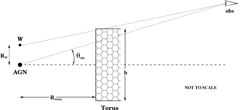
Figure 8: Cartoon of the proposed geometry of the warm reflector W and the dense, obscuring torus (see section 4.6). The cross section of the torus is shown here as rectangular, with full height $h$ and inner radius $R_{torus}$. The warm reflector $W$ is shown at radius $R_{W}$ from the AGN, and is positioned such that the line-of-sight to the observer just skims the surface of the torus. See Table 4 for properties of the warm reflector. The inclination angle of the observer $\theta_{obs}$ is measured with respect to the equatorial plane of the torus.

The covering fraction of the thickest part of the torus may also be estimated. In order to provide a significant “cold reflection” signal, the reflecting gas must be at least Compton thick. Consequently, it is only the thickest part of the torus that may contribute to this part of the X-ray spectrum. We have just seen that its transverse size is $\sim 0.1$ pc. Two pieces of evidence indicate that its distance from the nucleus is $\simeq 0.5$ pc. The VLBA images of Gallimore et al. (1997) stretch to radial distances $\simeq 0.6$ pc. Because the measured brightness temperature is $\sim 10^{6}$ K, the source of radio flux cannot be part of the torus, making its inner radius at least this large. VLBA maser observations, on the other hand, show that there is cool molecular gas as close as $\simeq 0.5$ pc from the nucleus (Greenhill et al.). On this basis, we suppose that $(\Omega/4\pi)_{torus}\simeq 0.1$.

The torus’s contribution to the “cold reflected” luminosity is the product of its covering fraction and its albedo. Combining the estimate of the previous paragraph with the cold reflection albedo computed by George & Fabian (1991) (2.2% for the 2$-$10 keV range), we would predict a torus contribution $\sim 7\times 10^{40}$ (L₀/10^43.5), which is comparable to L_N, our estimate of the X-ray reflection from neutral gas. Therefore, cold reflection from the inner edge of the torus could also contribute significantly.

4.7 Variability

As a consistency check, we note that between epochs 1 and 2, the total observed flux (and hence luminosity L_obs) decreased by a factor of 0.8, while L₀ and L_W ($=$ L_I) are inferred to have decreased by $\approx$0.2 dex, or by a factor of 0.63. This can be accomplished if L_I/L${}_{obs}=$ 0.54, assuming the cold reflector luminosity L_N did not vary. We note that for our joint (neutral$+$ionized reflection) fits described in section 4.6, L_I/L_obs is 0.72 for the optically thin warm reflector, and 0.58 for the optically thick warm reflector. Given the uncertainties of the fluxes used to estimate these fractions, and the shortcomings of the XSPEC ionized reflection models, the fractions are consistent with each other. The observational result from the joint fit implies that the X-ray emission from the warm reflector contributes $\sim$60-70% of the total observed luminosity.

4.8 A Consistent Model for the X-ray Reflectors

Many potential problems discussed here can be alleviated if the intrinsic X-ray luminosity of the AGN L${}_{0}\lesssim$ 10^43.5 erg s^-1. If L${}_{0}\approx$ 10^43.0 erg s^-1, the covering factor and filling factor of the warm reflector then become large enough to be consistent with equation $(3)$: $R_{W}/l_{W}\sim$ 1. This would also imply that the maximum X-ray reflection fraction f${}_{refl}\lesssim$ 0.01, which is comparable to the reflection factor for optical and UV light. The best-fit spectral models include a Compton reflection component, either from optically thick ionized gas, or from optically thick neutral gas. Therefore, if the optical depth of the ionized gas in the warm reflector is low enough so that a Compton “hump” is not present, reflection from optically thick neutral gas is needed. The torus can easily produce this cold reflection component, but the coronal gas in the NLR may also contribute (if $\tau_{Th}\gtrsim$ 1).

5 Implications and Conclusions

We propose that the 6.7/6.97 keV line emitting region and the previously unidentified warm, ionized reflector in NGC 1068 are indeed the same region. Approximately 2/3 of the total observed 2$-$10 keV X-ray emission comes from the warm reflector, which is located $\lesssim$0.2 pc from the AGN. The geometrical and physical properties of the warm reflector (Table 4) are quite different from those of the optical/UV reflector (e.g. Miller et al. 1991).

The warm X-ray reflector should reflect optical and UV light; however, no such emission is seen in HST images at the location of the proposed nucleus (e.g., Capetti et al. 1995). This suggests that the dust optical depth toward the nucleus is high enough to block the UV and optical light, but the equivalent X-ray column is not large enough to block the harder X-ray emission. Equivalent columns up to $\sim$10²² cm^-2 are allowed when fitting the X-ray models to the ASCA/RXTE/BeppoSAX data, so such a scenario is feasible from the X-ray point of view. We can achieve this scenario if the torus is viewed edge-on so that the line-of-sight toward the nucleus skims the edge of the torus (see Figure 8).

We estimate that $\sim$ 1/3 of the total observed 2$-$10 keV X-ray emission is reflected by optically thick, neutral reflectors. See Figure 9 for a cartoon illustrating the possible reflection regions.

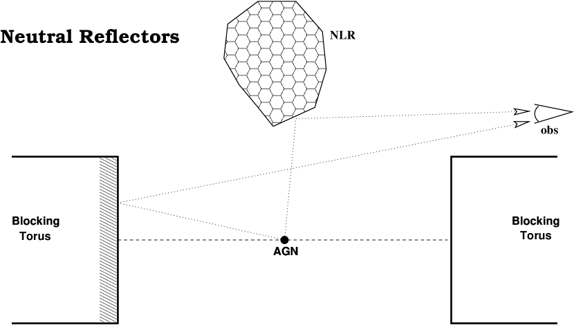
Figure 9: Cartoon of the two optically-thick ‘cold’ reflection regions: the inner surface of the dense, obscuring torus, and the optical reflection region (the inner NLR), located $\sim$30 pc from the AGN (Capetti et al. 1995). The shaded region of the torus illustrates that only a fraction ($\lesssim$ 0.5) of the inner surface of the torus reflects X-rays toward the observer. The coronal gas in the inner NLR has a moderately low ionization parameter ($\xi\sim$ 50) and may be optically thick to electron scattering, and therefore could also be a “cold” X-ray reflector.

If the coronal gas in the NLR is Compton thick, it is possible that all of the cold reflection component is from the NLR. We estimate a covering factor of $\approx$0.15 for the inner NLR, and $\sim$0.1 for the inner surface of the torus. Thus, either of these two regions could contribute significantly to the observed cold reflection component. Likewise, the 6.4 keV Fe emission line could originate from either of these regions.

VLBA observations of NGC 1068 (Gallimore et al. 1997) show that the size, radius and density of the radio-emitting clumps at the inner edge of the torus ($R\approx$ 0.6 pc, height $h\lesssim$ 0.1 pc) are very similar to those of our proposed warm reflector. If the warm reflector does indeed have a density $\gtrsim$10⁶ cm^-3 and a spherical volume of diameter $\sim$0.1 pc, and is at temperature of $\sim$0.1-1 keV, the emission measure will be large enough to see thermal bremsstrahlung radio emission (cf. Gallimore et al. 1997). However, since the emission $\propto$ n², values of $n$ below a few $\times$ 10⁵ (e.g., if D(NGC 1068) $<$ 14.67 Mpc) would force the bremsstrahlung luminosity below Gallimore et al.’s detection limit. It is worth noting that since the morphology of the radio clumps of S1 are not co-linear (as one would expect from an unwarped, edge-on disk/torus), it is quite possible that one of the clumps is in the Gallimore et al. radio image is the primary warm X-ray reflector.

How does our proposed warm reflector region fit in with the AGN paradigm? Krolik & Kriss (1995) suggest that the “warm absorbers” seen in type 1 AGN may be associated with the warm reflection region. Typical ionization parameters associated with the warm absorbers are $\xi\sim$ 10$-$100 erg cm s^-1 (e.g., Reynolds 1997, Kaspi et al. 2001), which is much lower than the values we find ($\xi\sim$ 10³). In principle, there could be clouds with different densities and mean ionization parameters in each of these regions, which could be responsible for the warm absorbers see in AGN X-ray spectra. One possibility is that the more highly ionized, inner regions of the warm reflector clouds reflect X-rays toward our line of sight, while the more weakly ionized, outer regions of the clouds cause the warm, ionized edges.

We suggest the existence of ionized, warm reflector gas clouds distributed within a radius of $\sim$0.2 pc. The highly ionized gas in this region produces an Fe K edge near 8.6 keV in the reflected nuclear spectrum, as well as both the observed 6.7 keV and 6.97 keV emission lines. Cold reflection, required to model the observed Compton reflection hump, originates from optically thick “cold” gas in the inner NLR and/or from the inner surface of the torus. Our data and proposed models are most consistent with an intrinsically X-ray weak AGN with L${}_{0}\approx$ 10^43.0 erg s^-1.

Table 1: Log of X-ray Spectral Observations of NGC 1068

Epoch	Dataset	ID	Observation Dates	Exp. Time	Detector
			(YYMMDD)	(ks)
0	ASCA1	70011000	930724$-$930725	21.8	S0
1	ASCA2	74034000	960815$-$960818	93.8	S0
1	RXTE	10322	960816$-$960819	48.3	PCA
2	SAX1	50047001	961230$-$970103	100.8	MECS
3	SAX2	50047002	980111$-$980112	37.3	MECS

Table 2: Epoch 1 Simple Continuum Model Fits: ASCA2$+$RXTE$+$SAX1/PDS

Model		$\Gamma$	R	$\chi^{2}$/dof	Notes
Fe K Complex fit Empirically with Four Fixed Gaussian Lines
1	Abs.P.L.	1.68	…	375.6/322	N${}_{H}=$ 1.0 $\times$ 1023 cm-3
2	P.L.$+$Edge	1.04	…	343.8/321	E${}_{edg}=$ 8.60 keV, $\tau_{edg}=$ 0.64
3	N.Refl.	1.44	1.19	401.2/322
4	I.Refl.	1.56	4.53	312.6/321	$\xi=$ 1798
Fe K Complex fit with Four Narrow Gaussian Lines
1	Abs.P.L.	1.43	…	370.2/318	N${}_{H}=$ 4.97${}_{-3.28}^{+3.11}$ $\times$ 1022 cm-2
		1.29-1.57			N$=$ 7.96${}_{-2.41}^{+3.29}$ $\times$ 10-4 photons keV-1 cm-2 s-1
2	P.L.$+$Edge	1.06	…	333.3/317	E${}_{edg}=$ 8.63${}_{-0.21}^{+0.23}$ keV, $\tau_{edg}=$ 0.54$\pm$0.14
		1.01-1.13			N$=$ 3.67${}_{-0.35}^{+0.45}$ $\times$ 10-4 photons keV-1 cm-2 s-1
3	N.Refl.	1.46	1.48	366.9/318
		1.31-1.66	0.52-3.53		N$=$ 6.31${}_{-1.15}^{+1.70}$ $\times$ 10-4 photons keV-1 cm-2 s-1
4	I.Refl.	1.54	4.07	313.4/317	$\xi=$ 1840${}_{-1020}^{+3160\tablenotemark{c}}$ erg cm s-1
		1.36-1.69	2.69-7.11		N$=$ 4.75${}_{-1.03}^{+0.96}$ $\times$ 10-4 photons keV-1 cm-2 s-1

Table 3: Fe K line fluxes for Epochs 1 and 2 (Narrow-Line Model)

Model and Parameters					Line Fluxes (10-5 photons cm-2 s-1)				$\chi^{2}$/dof
					6.21	6.4	6.7	6.97
					(keV)	(keV)	(keV)	(keV)
	Epoch 1    (see Table 2)
1					2.38	4.76	3.39	1.79
					1.79-2.98	4.10-5.41	2.86-3.94	1.38-2.21
2					2.38	4.67	3.40	1.52
					1.82-2.93	4.03-5.32	2.86-3.93	1.11-1.94
3					2.66	4.64	3.38	1.98
					2.10-3.21	3.99-5.29	2.84-3.92	1.57-2.39
4					2.02	4.71	3.34	1.03
					1.47-2.59	4.07-5.36	2.82-3.89	0.61-1.46
	Epoch 2    (Epoch 2 Continuum Model Fixed at Epoch 1 Parameters –
	CONSTANT power-law norm)
1					0	4.45	5.84	0.18	555.1/420
					$<$0.23	3.68-5.22	4.77-6.75	$<$0.90
2					0	4.45	5.96	0	501.4/420
					$<$0.24	3.73-5.21	4.90-6.69	$<$0.70
3					0	4.78	5.63	0.52	529.9/420
					$<$0.27	4.00-5.55	4.56-6.70	$<$1.23
4					0	4.25	5.57	0	502.9/420
					$<$0.19	3.52-4.96	4.82-6.30	$<$0.31
	Epoch 2    (Epoch 2 Continuum Model Fixed at Epoch 1 Parameters –
	VARIABLE power-law norm)
1	N=6.45				0	5.51	5.28	1.13	480.5/418
	5.89-6.74				$<$0.52	4.62-6.32	4.20-6.36	0.39-1.88
2	N=2.98				0	5.50	5.39	0.96	429.5/417
	2.56-3.11				$<$0.57	4.23-6.30	4.01-6.47	0.22-1.70
3	N=5.17				0	5.73	5.13	1.36	465.2/418
	4.38-5.40				$<$0.64	4.23-6.53	3.62-6.21	0.57-2.10
4	N=3.82				0	5.14	5.65	0.45	420.2/419
	3.41-3.99				$<$0.47	4.28-5.95	4.56-6.71	$<$1.20
	Epoch 2    (Epoch 2 Continuum Model Parameters Allowed to Vary)
1	$\Gamma$=1.55				0	5.55	5.24	1.22	482.0/419
	1.53-1.59				$<$0.50	4.65-6.34	4.17-6.33	0.46-1.95
1	NH=10.0				0	4.99	5.52	0.64	503.8/419
	8.7-11.3				$<$0.34	4.20-5.77	4.43-6.59	$<$1.37
1	$\Gamma$=1.56	NH=4.56			0	5.57	5.23	1.24	482.0/418
	1.51-1.61	2.34-6.84			$<$0.51	4.67-6.37	4.16-6.32	0.48-1.99
1	$\Gamma$=1.24	NH=0	N=3.89		0	5.72	5.24	1.25	472.5/417
	1.12-1.37	$<$1.99	3.11-5.13		$<$0.67	4.70-6.52	4.16-6.32	0.50-1.99
2	$\Gamma$=1.18				0	5.51	5.37	1.02	430.3/419
	1.15-1.22				$<$0.54	4.59-6.31	4.29-6.45	0.28-1.77
2	$\tau_{edg}$=0.84				0	4.45	5.96	0	496.6/419
	0.60-1.12				$<$0.24	3.73-5.22	4.90-6.69	$<$0.70
2	$\Gamma$=1.14	$\tau_{edg}$=0.41	N=3.40		0	5.55	5.35	1.04	428.1/416
	1.03-1.26	0.16-0.70	2.53-4.16		$<$0.58	4.51-6.35	4.24-6.44	0.29-1.79
3	$\Gamma$=1.58				0	5.72	5.00	1.46	462.5/417
	1.55-1.67				$<$0.65	4.36-6.60	3.59-6.16	0.72-2.21
3	$\Gamma$=1.68	R=2.7			0	5.15	4.51	1.33	462.8/417
	1.50-1.88	$<$10.1			$<$0.68	4.25-6.65	3.51-6.15	0.64-2.24
3	$\Gamma$=1.68	R=5.0	N=6.30		0	5.58	5.07	1.33	465.5/417
	1.40-1.95	1.4-12.9	4.47-8.03		$<$0.53	4.51-6.40	3.93-6.15	0.59-2.07
4	$\Gamma$=1.65				0	5.16	5.61	0.53	422.6/419
	1.63-1.69				$<$0.45	4.31-5.96	4.53-6.69	$<$1.28
4	$\Gamma$=1.49	R=2.41	$\xi$=300		0	5.42	5.45	0.82	414.9/417
	1.38-1.63	0.94-5.41	$<$2130		$<$0.56	4.44-6.27	4.00-6.55	$<$1.97
4	$\Gamma$=1.62	R=3.92	$\xi$=0	N=5.95	0	5.58	5.12	1.26	414.0/416
	1.38-1.82	1.28-7.97	$<$4550	3.70-7.55	$<$0.41	5.00-6.20	4.34-6.31	0.20-2.10

Table 4: Ionized Warm Reflector Properties

Property		Value	Unit
$l_{W}$	Diameter	$\lesssim$ 0.2	pc
$n_{W}$	Density	$\gtrsim$ 105.5	cm-3
$log~{}\xi_{W}$	Ionization Parameter	3.45$-$3.75	$log$(erg cm s-1)
$R_{W}$	Radius (from AGN)	$\sim l_{W}$

References

- Antonucci (1993) Antonucci, R. R. J. 1993, ARA&A, 31, 473
- Antonucci & Miller (1985) Antonucci, R. R. J., & Miller, J. S. 1985, ApJ, 297, 621
- Beiersdorfer et al. (1993) Beiersdorfer, P., Phillips, T., Jacobs, V. L., Hill, K. W., Bitter, M., von Goeler, S., & Kahn, S. M. 1993, ApJ, 409, 846
- Capetti et al. (1997) Capetti, A., Axon, D. J., & Macchetto, F. D. 1997, ApJ, 487, 560
- Capetti et al. (1995) Capetti, A., Macchetto, F., Axon, D. J., Sparks, W. B., & Boksenberg, A. 1995, ApJ, 452, L87
- Crenshaw et al. (2000) Crenshaw, D. M., & Kraemer, S. B. 2000, ApJ, 532, 256
- Dickey & Lockman (1990) Dickey, J. M., & Lockman, F. J. 1990, ARA&A, 28, 215
- Elvis et al. (1994) Elvis, M. et al. 1994, ApJS, 95, 1
- Feldman et al. (1980) Feldman, U., Doschek, G. A., & Kreplin, R. W. 1980, ApJ, 238, 365
-
Fiore et al. (2001)
Fiore, F., Giommi, P., &
Guainazzi, M. 2001, NFI Cross-Calibration,
http://www.ias.rm.cnr.it/ias-home/sax/software/cookbook/cross_cal.html - Gallimore et al. (1997) Gallimore, J. F., Baum, S. A, & O’Dea, C. P. 1997, Nature, 388, 852
- George & Fabian (1991) George, I. M., & Fabian, A. C. 1991, MNRAS, 289, 443
- Ghisellini et al. (1994) Ghisellini, G., Haardt, F., & Matt, G. 1994, MNRAS, 267, 743
- Iwasawa et al. (1997) Iwasawa, K., Fabian, A. C., Matt, G. 1997, MNRAS, 289, 443
- Kaspi et al. (2001) Kaspi, S. et al. 2001, ApJ, 554, 216
- Kinkhabwala, A. et al. (2002) Kinkhabwala, A., et al. 2002, in “New Visions of the X-ray Universe in the XMM-Newton and Chandra Era,” (ESTEC: Noordwijk), ed. F. Jansen (astro-ph/0203021)
- Kishimoto (1999) Kishimoto, M. 1999, ApJ, 518, 676
- Koyama et al. (1980) Koyama, K., Inoue, H., Tanaka, Y., Awaki, H., Takano, S., Ohashi, T., & Matsuoka, M. 1989, PASJ, 41, 731
- Kraemer et al. (2000a) Kraemer, S. B., & Crenshaw, D. M. 2000, ApJ, 532, 247
- Kraemer et al. (2000b) Kraemer, S. B., & Crenshaw, D. M. 2000, ApJ, 544, 763
- Krolik & Kallman (1987) Krolik, J. H., & Kallman, T. R. 1987, ApJ, 320, L5
- Krolik, Madau & Zycki (1994) Krolik, J. H., Madau, P., & Zycki, P. T. 1994, ApJ, 420, L57
- Krolik & Kriss (1995) Krolik, J. H., & Kriss, G. A. 1995, ApJ, 447, 512
- Leahy & Creighton (1993) Leahy, D. A., & Creighton, J. 1993, MNRAS, 263, 314
- Levenson et al. (2001) Levenson, N. A., Weaver, K. A., & Heckman, T. M. 2001, ApJS, 133, 269
- Magdziarz & Zdziarski (1995) Magdziarz, P. & Zdziarski, A. A. 1995, MNRAS, 273, 837
- Marshall et al. (1993) Marshall, F. E., et al. 1993, ApJ, 405, 168
- Matt, Fabian & Ross (1993) Matt, G., Fabian, A. C., & Ross, R. R. 1993, MNRAS, 262, 179
- Matt, Brandt & Fabian (1996) Matt, G., Brandt, W. N., & Fabian, A. C. 1996, MNRAS, 280, 823
- Matt et al. (1997) Matt, G., et al. 1997, A&A, 325, L13
- Miller et al. (1991) Miller, J. S., Goodrich, R. W., & Mathews, W. G. 1991, ApJ, 378, 47
- Mulchaey et al. (1994) Mulchaey, J. S., et al. 1994, ApJ, 436, 586
- Mulchaey et al. (1992) Mulchaey, J. S., Mushotzky, R. F., & Weaver, K. A. 1992, ApJ, 390, L69
- Mushotzky (1982) Mushotzky, R. F. 1982, ApJ, 256, 92
- Nandra et al. (1997) Nandra, K., George, I. M., Mushotzky, R. F., Turner, T. J., & Yaqoob, T. 1997, ApJ, 477, 602
- Nandra & Pounds (1994) Nandra, K., & Pounds, K. 1994, MNRAS, 268, 405
- Netzer et al. (1998) Netzer, H., Turner, T. J., & George, I.M. 1998, ApJ, 504, 680
- Reynolds (1997) Reynolds, C. S. 1997, MNRAS, 286, 513
- Reynolds & Fabian (1995) Reynolds, C. S., & Fabian, A. C. 1995, MNRAS, 273, 1167
- Ogle et al. (2001) Ogle, P. M., Canizares, C., Dewey, D., Lee, J., & Marshall, H. 2001, in Mass Outflow in Active Galactic Nuclei: New Perspectives (ASP: Washington), ed. D. M. Crenshaw & S. B. Kraemer
- Pier et al. (1994) Pier, E. A., Antonucci, R., Hurt, T., Kriss, G., & Krolik, J. 1994, ApJ, 428, 124
- Seyfert (1943) Seyfert, C. K. 1943, ApJ, 97, 28
- Smith, Done & Pounds (1993) Smith, D. A., Done, C., & Pounds, K. A. 1993, MNRAS, 263, 54
- Turner & Pounds (1989) Turner, T. J., & Pounds, K. 1989, MNRAS, 240, 833
- Ueno et al. (1994) Ueno, S., Mushotzky, R. F., Koyama, K., Iwasawa, K., Awaki, H. & Hayashi, I. 1994, PASJ, 46, L71
- Verner et al. (1996) Verner, D. A., Ferland, G. J., Korista, K. T., & Yakovlev, D. G. 1996, ApJ, 465, 487
- Whittle (1992) Whittle, M. 1992, ApJS, 79, 49
- Wilson et al. (1992) Wilson, A. S., Elvis, M., Lawrence, A., & Bland-Hawthorn, J. 1992, ApJ, 391, L75
- Yaqoob et al. (2000) Yaqoob, T., & ASCA Team 2000, ASCA GOF Calibration Memo ASCA-CAL-00-06-02, v1.0 (06/07/00)