The Planetary Nebulae Spectrograph:
the green light for Galaxy Kinematics

Abstract

Planetary nebulae are now well established as probes of galaxy dynamics and as standard candles in distance determinations. Motivated by the need to improve the efficiency of planetary nebulae searches and the speed with which their radial velocities are determined, a dedicated instrument - the Planetary Nebulae Spectrograph or PN.S - has been designed and commissioned at the 4.2m William Herschel Telescope. The high optical efficiency of the spectrograph results in the detection of typically $\sim 150$ PN in galaxies at the distance of the Virgo cluster in one night of observations. In the same observation the radial velocities are obtained with an accuracy of $\sim 20$ km s^-1
note that due to archival restrictions the figures have been strongly compressed - please contact any of the authors for a better preprint

1 Introduction

The study of the internal dynamics of galaxies provides some of the best observational clues to their formation history and mass distribution, including dark matter, but much of the interesting information is inaccessible with conventional techniques. Stellar kinematics, the most important diagnostic, have generally been determined using absorption-line spectra of the integrated light, the surface brightness of which is such that only the inner parts of the galaxy can be observed in a reasonable amount of telescope time. In practical terms, it is hard to measure the integrated stellar spectra beyond $1-2R_{e}$ (the “effective radius”, which contains half the galaxy’s projected light). This is a serious limitation, because it is at larger radii that the gravitation of the dark matter halo is likely to dominate, and that the imprint of the galaxy’s origins are likely to be found in its stellar orbits.

Alternative diagnostics of the gravitational potential include measurement of the 21cm-wavelength emission from neutral hydrogen, observations of HII regions, and the observation of the motions of globular clusters and planetary nebulae. But neutral hydrogen and HII regions are effectively absent from early- type galaxies, and globular clusters, not surprisingly, have been found to be kinematically distinct from the stellar population which is of primary interest.

Planetary nebulae (PN) are part of the post-main-sequence evolution of most stars with masses in the range 0.8–8 M_⊙. Taking into account the duration of the PN phase itself, even in a galaxy with continuing star formation most observed PN will have progenitors in the range 1.5–2 M_⊙, corresponding to a mean age of $\sim 1.5$ Gyr. In the case of early-type galaxies the PN are drawn from the same old population that comprises most of the galaxy light.

PN are sufficiently bright to be detected in quite distant galaxies and their radial velocities are readily measured by a variety of techniques. Moreover, because they are easier to detect at large galactocentric radius where the background continuum is fainter, they represent the crucially important complement to absorption line studies. These properties make PN an ideal kinematic tracer for the outer parts of such galaxies, allowing the measurement of stellar kinematics to be extended out to typically $4-5R_{e}$.

A common and well-tested technique for obtaining the radial velocities of PN consists of a narrow-band imaging survey of [OIII] emission to identify candidates, followed by a spectroscopic campaign to obtain their spectra. This approach has in the past commonly resulted in low yields (see §3.1).

We have developed an alternative single-stage method, which uses narrow-band slitless spectroscopy. By obtaining two sets of data with the spectra dispersed in different directions (a technique we call “counter-dispersed imaging” or CDI), one can identify PN and measure their radial velocities in a single observation. The use of CDI by modifying existing instrumentation has been so successful that we decided to design and build a custom-made CDI spectrograph, with an overall efficiency improvement of about a factor of ten over a typical general-purpose spectrograph.

The organisation of this paper is as follows. In §2 we review the important observational characteristics of PN and discuss the implications of their luminosity function for the number of PN which can be detected. In §3 we introduce CDI and compare it with more traditional techniques. The PN.Spectrograph, which is the main subject of this paper, is presented in some detail in §4. As well as a complete technical discussion, and a short history of the project, this section includes some of the first images obtained with the instrument, following its recent successful commissioning. Further technical information is presented in three appendices.

2 Observation of extragalactic PN

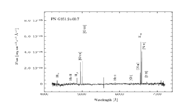
PN, which are unresolved objects at distances of 1 Mpc or more, can be detected by means of their strong characteristic emission lines (see Fig. 1). The narrowness of the lines (the intrinsic linewidth is usually less than 30km s^-1) makes it relatively easy to measure the radial velocities of the individual PN.

The brightest line is usually the 5007Å line of [O III] in which as much as 15% of the central star’s energy is emitted (Dopita et al., 1992). The PN brightness in this line is conventionally given in magnitudes as

$$m_{5007}=-2.5\log F_{5007}-13.74$$ (1)

where $F_{5007}$ is in erg cm^-2 s^-1 and the constant is such that a star of the same magnitude would appear to be equally bright when observed through an ideal V-band filter. The [O III] line consists of a doublet 4959/5007Å with the intensity ratio 1:3. Only the brighter component of the doublet (rest wavelength in air 5006.843Å) is included in the above magnitude. The absolute magnitude $M_{5007}$ is defined in the usual way.

Figure 1: A typical PN optical spectrum, showing the many emission lines visible in such a nebula, as well as the dominance of the [O III] line. Figure kindly provided by F. Kerber, ESO.

PN are found to have a well-behaved luminosity function $\Phi$ which can be approximated by (dropping the 5007 subscript)

$$\Phi(M)\propto e^{0.307M}[1-e^{3(M^{*}-M)}]$$ (2)

where the parameter $M^{*}$, defining a sharp bright-end cutoff to the luminosity function, was normalised using PN in M31 to $M^{*}$ = –4.48 (Ciardullo et al., 1989) and has since changed only slightly (Ciardullo et al., 2002a). The symbol $m^{*}$ is used for the apparent magnitude of the PNLF cutoff.

By fitting the above function to a (complete) sample of PN in a given galaxy a distance estimate can be made. This application of the PNLF, the characteristics of which are under constant review (see e.g. Ferrarese et al. (2000)), will not concern us further here, but knowledge of the shape of the PNLF is important in that it allows us to estimate the relative number of PN in a given system down to a certain magnitude limit (see below).

The absolute number of PN present in a stellar system is usually characterised by the number-density in the top dex (2.5 magnitudes) of the PNLF, normalised to bolometric magnitude, which takes a value

$$\alpha_{2.5}\sim 7-50\times(10^{9}L_{\sun,{\rm bol}})^{-1},$$ (3)

depending on the colour (Ciardullo et al., 1991) and luminosity (Ciardullo, 1995) of the galaxy. For practical purposes a number-density ($\beta_{2.5}$) normalised to the B-band luminosity is often used.

Eqn 2 can be used to compute the cumulative luminosity function. The results, normalised to $\alpha_{2.5}$, are shown in Table 1. This shows for example that to double the number of PN detected in a given galaxy with respect to a complete sample down to $M-M^{*}=2.5$ one needs to reach a limit nearly 1.5 magnitudes, or a factor 4 in flux, fainter.

As a numerical example we consider the Virgo galaxy NGC 4374, with an assumed distance of 15 Mpc and a foreground extinction of 0.2 mag. The brightest PN in this galaxy would be expected to have an apparent magnitude of $m^{*}_{5007}\simeq 26.6$, corresponding to an [O III] flux of $7.3\times 10^{-17}$ erg cm^-2 s^-1. This converts to a detection rate in the [O III] line of 0.7 photon per second for a 4m telescope with 30% system efficiency. For NGC 4374, $\alpha_{2.5}=16.7$ (Jacoby et al., 1990), and with the appropriate bolometric correction (BC = $m_{\rm bol}-m_{V}$ = -0.83) and colour index (B-V = 0.97) this corresponds to $\beta_{2.5}=47.7$. Correcting the apparent magnitude ($m_{\rm B}=10.3$) for distance and extinction gives $M_{\rm B}=-20.8$, corresponding to $32.5\times 10^{9}L_{\sun,{\rm B}}$. Thus one would expect $\sim 1550$ PN in the top dex of the luminosity function or, using Table 1, $\sim 710$ down to the magnitude limit $m^{*}_{5007}=28.1$.

By definition half of these would fall within one effective radius of the centre, where the noise contribution from the galaxy light is very significant, and be hard to detect. For NGC 4374 the B-band background light is 22.2 mag arcsec^-2 at $1R_{e}$, which corresponds to 50% of the dark night sky background at a good observing site.

To put the above number of PN in perspective, note that $\sim$1000 radial velocities are necessary to nonparametrically constrain the dynamical properties of a hot stellar system (Merritt and Saha (1993), Merritt and Tremblay (1993)). However, early-type galaxies normally have integrated light kinematical measurements available to $\sim 1R_{e}$, the addition of which dramatically decreases the number of discrete velocity measurements needed. In such cases, $\sim$100–200 velocities can place strong constraints on a galaxy’s mass distribution (Saglia et al. (2000), Romanowsky and Kochanek (2001)). If 200 PN velocities are measured outside 1 $R_{e}$, $\sim$50 will be outside 3 $R_{e}$, a sample that can reliably constrain the rotational properties of the galaxy’s outer parts (Napolitano et al. (2001)).

Table 1: The cumulative PN luminosity function (top row) as a function of magnitude (bottom row).

	0.00	0.08	0.24	0.46	0.71	1.00	1.34	1.74	2.21	2.75	3.39
$M-M^{*}$	0.0	0.5	1.0	1.5	2.0	2.5	3.0	3.5	4.0	4.5	5.0

3 Observing techniques

To study the kinematics of extragalactic PN, there are two aspects: finding the PN and obtaining their radial velocities. In the following sections we discuss the techniques applied to this problem so far. Simple formulae are given for the S/N achieved with each technique, and then used to compute the integration time required to reach $S/N=10$ for a PN with given magnitude. This is a reasonable benchmark since experiments show that detection completeness varies from nearly 100% at $S/N\geq 9$ to 0% at $S/N=4$ (Ciardullo, 1987). We compute the noise as the quadratic sum of poisson noise from the object, sky background, and detector read out. We adopt the notation of Table 2 and the default values therein, unless otherwise specified.

The “system efficiency” which is quoted for multi-object spectroscopy (MOS) and other techniques is based on typical limiting magnitudes actually achieved with current instrumentation at 4-m class telescopes. By definition it includes telescope, filter and detector efficiency as well as the efficiency of the instrument proper, but it should be stressed that light loss due to the finite size of the fibre or slit, and hence also astrometric, pointing, and tracking errors affect the performance of MOS instruments. This can lead to values of the system efficiency which are smaller by a factor of two or more than the nominal optimum instrument performance.

In these and other calculations in the paper we include atmospheric losses of 0.15 mag corresponding to an airmass of 1.0 at a good observing site.

Table 2: Parameters used in the computation of integration time required for a given S/N.

Symbol	Description
$S/N$	final signal-to-noise ratio for the detection of a PN
	against a background, including all noise contributions
FWHM	the FWHM of the seeing point-spread-function (default 1″)
${A_{\rm psf}}$	in imaging, the area   $\pi(\frac{2}{3}{\rm FWHM})^{2}$ over which the $S/N$ is calculated
$F_{\rm PN}$	detected [O III] flux from the object in photons/sec
$T$	total integration time, in seconds
${T_{\rm on}}$	integration time spent on-band, in seconds
$F_{\rm back}$	total detected background flux   in photons/sec/Å/arcsec2
$B$	bandwidth of the [O III] band-pass filter (default 30.0Å)
${A_{\rm fibre}}$	in a fibre-fed spectrograph, the effective size of the fibre,
	as projected onto the sky (default 1.5 arcsec2)
$\Delta_{\lambda}$	in a spectrograph, width of a resolution element (default 3.0Å)
$n_{p}$	in imaging, number of pixels over which the integration is calculated
	(default ${A_{\rm psf}}*9$)
$n_{p}$	in spectroscopy, number of pixels over which the integration is calculated
	(default 9)
$n_{r}$	number of times the CCD is readout per integration
	(default 2 per hour)
$r$	read-noise, converted to photons (default 4.0)

3.1 Survey/multi-object spectroscopy

Most of the PN work on external galaxies has been done by first performing an imaging survey to obtain a sample of PN, and then following this up with multi-fibre or multi-slit spectroscopy of the individual objects to obtain their radial velocities (Hui et al., 1995).

Detection of the PN in [O III] emission is usually done by comparing images made with on-band and off-band filters (Jacoby et al., 1990), which allows PN candidates to be distinguished from foreground stars. For maximum sensitivity, the on-band filter should only be wide enough to accommodate the expected range of velocities, while the off-band filter can be broader. The positions of the PN must be determined to at least 0.5 arcsec precision in order to set up a subsequent observing campaign with standard multi-object spectroscopy (MOS).

For the detection of a PN in a narrow-band survey

$$S/N=F_{\rm PN}{T_{\rm on}}/\sqrt{F_{\rm PN}{T_{\rm on}}+{A_{\rm psf}}F_{\rm back}B{T_{\rm on}}+n_{p}n_{r}r^{2}}$$ (4)

where the symbols are defined in Table 2. The assumption is made that the off-band integration time ($T-{T_{\rm on}}$) is chosen such as to reach the same level of sky background (owing to the wider bandpass the image can be obtained relatively quickly). For useful S/N values, the read-noise is usually negligible.

As an illustration, consider the case of a survey carried out at a telescope of 4.0m diameter. The overall detection efficiency is assumed to be 0.4, and $T$ is divided between narrow-band and broad-band imaging in the ratio 80:20 (${T_{\rm on}}=0.8\times T$). The assumed background (see Table 2) corresponds to $F_{\rm back}=0.20$ photons/sec/Å/arcsec² for this case. The goal is to detect objects down to $m_{5007}=28$ with ${\rm S/N}~{}\sim 10$. Equation 4 with default parameters indicates that this can be achieved in $T=6.2$ hours.

The spectroscopy can be done efficiently with fibre or multislit spectroscopy, and the detection of the [O III] line is usually dominated by photon noise. For example, for fibre spectroscopy at spectral resolution $\Delta_{\lambda}$, this being the bandwidth corresponding to the projected width of the fibre in the spectra,

$$S/N=F_{\rm PN}T/\sqrt{F_{\rm PN}T+{A_{\rm fibre}}F_{\rm back}\Delta_{\lambda}T+n_{p}n_{r}r^{2}}$$ (5)

For this case, the system efficiency measured in practice (see § 3) is usually in the range 0.05-0.1, and here we adopt 0.1. With similar observing parameters to the previous example, and default values for $\Delta_{\lambda}$ and ${A_{\rm fibre}}$, the multi-object spectrograph should then return spectra with S/N $\approx 10$ for a $m_{5007}=28$ object in about $T=3.3$ hours.

Since several fibre configurations might be required to obtain all of the spectra (as a result of limitations on the number of fibres or on their positioning) we must multiply $T$ by some factor, typically $\sim 2-4$. Total time for the project, even with these ideal assumptions, is thus $\sim 13-19$ hours. However, as discussed in §3.4, several practical problems arise in the MOS follow-up to narrow-band imaging, significantly reducing the yield of PN velocities obtained.

3.2 Fabry-Perot interferometry

A Fabry-Perot system produces a cube of narrow-band images and is in principle well suited to observing extragalactic PN. Its large field of view (10′ at a 4-m telescope is typical) can encompass typical galaxies out to five effective radii at the distance of the Virgo Cluster. Tremblay et al. (1995) used this technique to study the PN in the SB0 galaxy NGC 3384.

The theoretical signal-to-noise for the detection of an emission-line object in the appropriate step from a wavelength scan in which a total bandpass $B$ is scanned over $N$ resolution elements is

$$S/N=(F_{\rm PN}T/N)/\sqrt{(F_{\rm PN}T/N)+{A_{\rm psf}}F_{\rm back}\ (B/N)(T/N)+2n_{p}r^{2}}$$ (6)

where now $n_{r}=1$ is assumed since the integration time per step is usually short. The factor 2 in the read-noise term allows for the fact that the actual step size needs to be such that there are two steps per resolution element.

When sky noise dominates, the Fabry-Perot procedure is equivalent to observing each planetary nebula by direct detection through an ideal filter (of bandwidth $B/N$) for time $T/N$, and the corresponding $S/N$ is similar to that of narrow-band imaging (with bandwidth $B$ and time $T$). However both read out noise and the poisson noise of the object being detected reduce the $S/N$ significantly. Neverthless, since the Fabry-Perot requires no follow-up spectroscopy, it is competitive with other techniques.

With other parameters as before we now assume an overall detection efficiency of 0.3 including the Fabry- Perot etalon, and $N=40$, giving a nominal resolution element of about 45 km s^-1. Equation 6 then shows that 21.6 hours observing is required to cover the passband and to reach $S/N\sim 10$ in each resolution element for the same magnitude limit as before. In the absence of read-noise, the same limit would be reached in about 13 hours.

3.3 Counter-dispersed imaging (CDI)

Figure 2: Left panel: illustration of counter-dispersed imaging - the arrow denoting the dispersion direction. Right panel: (left) the corresponding images of a star and planetary nebula shown schematically.

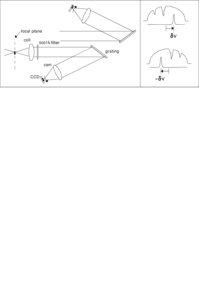
CDI, which has antecedents in the work of Fehrenbach (e.g. Fehrenbach (1947)), is illustrated schematically in Fig. 2. The left panel shows that two images of a given field must be taken through a slitless spectrograph equipped with a [O III] filter. The field is identical in the two cases but the dispersion direction is reversed. This can be done simply by rotating the spectrograph sequentially between position angles differing by 180^∘.

As shown in the right-hand panel of the Figure, stars in the field appear in the images as short segments of spectra whose extent depends upon the dispersion of the grating and on the filter bandwidth. The PN, on the other hand, are detected only on the basis of their single emission line and thus appear as point sources. The exact position at which each PN is detected in the slitless images depends upon the actual position of the PN on the sky and its precise wavelength. As the two images are counter-dispersed it can readily be seen that, after matching up the detected PN in pairs in the final images, one directly obtains relative velocities and positions. The velocities can be put on an absolute scale if the slitless observations include an arc line calibration through a slit. This discussion of the velocity solution is somewhat oversimplified, and we return to this topic later (§4.4) in more detail.

For a detected PN the S/N in each image takes the form

$$S/N=(F_{\rm PN}{T_{\rm on}})/\sqrt{F_{\rm PN}{T_{\rm on}}+{A_{\rm psf}}F_{\rm back}B{T_{\rm on}}+n_{r}n_{p}r^{2}}$$ (7)

where the total observing time $T$ is split between the two position angles (${T_{\rm on}}=T/2$). With the same parameters as before except for an overall system efficiency of 0.3 (somewhat less than for narrow-band imaging because of the presence of a grating in the beam), each CDI image achieves ${\rm S/N}\approx$ 10 in $T=13.1$ hours. In the case of simultaneous CDI (§4.1) there will be twice as many images and therefore more read-noise, but this has negligible effect.

3.4 Advantages of CDI

The results of the previous sections are summarised in Fig. 3, which shows the S/N reached with a 4.0m diameter telescope by different techniques - CDI, direct imaging (not including the follow-up spectroscopy), and Fabry-Perot spectroscopy - as a function of integration time. The same parameters were used as before.

Figure 3: Attained signal to noise ratio as function of telescope time, for three different techniques of searching for planetary nebulae. Solid line: counter-dispersed imaging (PN.S); dashed line: Fabry-Perot; dotted line: narrow-band imaging (not including spectroscopic follow-up). For each, three curves are plotted, referring (top to bottom) to $m_{5007}=25$, 28, and 30.

As can be seen, the FP technique is inferior except for very faint sources, being more sensitive to read noise on the one hand, and on the other hand not as efficient as the other techniques for the bright sources which are not background limited.

Narrow-band imaging is somewhat more efficient than CDI, but the former still requires the spectroscopic follow-up work. Multi-object spectroscopy can in principle be very efficient, but the need for several MOS configurations alone will usually mean that a campaign based on surveying and follow-up spectroscopy will require more total telescope time for a given yield than would be required with CDI.

Moreover there are additional problems. The imaging and the spectroscopy are rarely carried out on the same instrument, or even the same telescope. Observing time must be obtained twice, possibly at different telescopes and usually in different seasons, with greater risk of poor weather and incomplete data sets. Astrometric errors in transferring from the survey position to the fibre position sometimes mean that the spectrum is not obtained (e.g. Arnaboldi et al. (1996) recovered only 19 PN spectra from a survey set of 141 in NGC 4406), and the yield is further reduced by the fact, recently discovered (Kudritzki et al. (2000), Arnaboldi et al. (2002)), that the sample from the narrow-band imaging technique is sensitive to contamination from misidentified continuum objects.

CDI can be done with one instrument and at one telescope, and although still vulnerable to the possibility of incomplete or inhomogeneous datasets as a result of changes in observing conditions, this problem can be eliminated by obtaining the CDI images simultaneously.

In CDI the relative velocities are extremely accurate, being determined by the centroiding of images on the stable medium of a CCD. The radial velocity precision is comparable to that of fibre spectrographs of similar spectral resolution. We note that multi-slit velocities are typically less precise: they are subject to significant errors resulting from object positioning within the slit.

Accurate photometry requires, amongst other things, knowledge of the filter profile. Generally manufacturer’s curves are generated with very high focal ratio beams and at laboratory temperatures. In CDI the filter profile can be determined from the dispersed images of foreground stars, at the focal ratio and temperature appropriate to the observations and as a function of position on the detector, so accurate photometry is possible. It is more difficult to determine the filter characteristics in direct imaging mode. Note also that with the assumptions made earlier, that a given object is detected in each image with the same value of S/N, the effective integration time on which PN fluxes are based in CDI is twice that of the narrow-band image.

One disadvantage of CDI, relative to more conventional spectroscopic techniques, is its limited ability to distinguish between PN and other emission-line objects like unresolved HII regions, Ly$\alpha$ emitters at redshift $z\sim 3.1$ and starburst galaxies at $z\sim 0.3$. However on average the number of expected high-$z$ contaminants in a field of our size (100 arcmin²) is only 2-3 (Ciardullo et al., 2002b), and these can usually be recognised by their large linewidth, which the PN.S has some ability to resolve. Further identification of these objects, and HII regions (rare in early-type galaxies) could be accomplished with an Halpha arm (see §7).

3.5 Results with CDI

The CDI idea was systematically investigated in 1994-95 by Douglas and Taylor (at that time both at the Anglo-Australian Observatory (AAO)) and Freeman. The first published experiments, confirming with high accuracy positions and velocities for PN which had previously been detected in Cen A, were carried out by removing the slit unit from the RGO spectrograph at the 3.9 m AAT (Douglas and Taylor, 1999). Subsequently the ISIS spectrograph at the 4.2 m WHT was used between 1997 and 2000 to obtain the kinematics of M94 (Douglas et al., 2000) and several S0 galaxies, and in 1998 an attempt was made to reach planetaries in the E5 galaxy NGC 1344 using CDI at the ESO 3.6 m. In these cases the counter-dispersed images were obtained by rotating the spectrograph. We note the related technique used by Méndez et al. (2001), who used an undispersed narrow-band image and a single slitless dispersed image to detect extragalactic PN and to measure their velocities.

The principal gain in designing a dedicated instrument is the possibility of increasing both the optical efficiency and field size. The use of such an instrument can enable projects to be carried out at a 4m telescope which would otherwise require an 8m telescope with general-purpose instrumentation.

4 The PN.Spectrograph project

These considerations led us to consider the construction of a purpose-built instrument. In this section we present first the design philosophy, then optical and mechanical details, before returning to the issue of calibration. A chronology of the PN.Spectrograph project is given, and the first observational results are presented.

4.1 Design considerations

An important and unique driver of our PN.S design was that it should deliver simultaneous counter-dispersed imaging, avoiding the need to rotate the instrument between the two position angles. As described later in this section, this was achieved by using a matched pair of gratings and cameras, creating what is in effect two spectrographs back-to-back. The increased complexity is compensated by several advantages: the CDI data sets are always matched in quality and integration time, and the velocity determination is more accurate since all calibrations are done at the same time. Differential flexure is less and can be more easily monitored.

The original PN.S design studies were for an f/15 instrument to operate at the Anglo-Australian Telescope (3.9m aperture) and/or the ESO VLT (8m). However, driven by considerations of cost and telescope access, we decided instead to design the instrument to operate at both the UK/NL William Herschel Telescope (4.2m) and the Italian Telescopio Nazionale Galileo (3.5m), both located on the island of La Palma. The TNG is based on the ESO NTT and has two f/11 Nasmyth focal stations with instrument derotators. The WHT also has a Nasmyth platform for interchangeable instrumentation but there the field of view is rather restricted owing to the use of an optical derotator. We therefore opted for the WHT f/11 Cassegrain focus with instrument derotator. This station also includes a suite of calibration lamps. Consistent with this choice of telescopes and focal stations, the field-of-view was chosen to be $\sim 10$′ square. To be able to optimize the throughput as much as possible, we designed for the smallest wavelength range consistent with the range of galaxy systemic velocities likely to be of interest ($\pm 1800$ km s^-1).

The most critical component in maximising the instrument efficiency over a narrow wavelength range is the grating. The performance of standard commercial blazed gratings were examined with the assistance of computer codes.

For the CDI detection of PN the dispersion should not be too high because of three effects: firstly, field is lost since PN whose images are dispersed outside either of the counter-dispersed frames cannot be used, secondly the dispersed images of foreground stars obliterate a fraction of the field, and thirdly the increased separation between CDI pairs increases the degree of confusion, making it more likely that some objects cannot be unambiguously paired up. On the other hand, the dispersion should be high enough for the required velocity precision. Calculations show that it should be possible to centroid a well-sampled PSF with given $S/N$ to an accuracy of ${\delta_{\rm psf}}\sim\frac{0.7}{S/N}{\rm FWHM}$ (see Appendix 9). Given a detection (in each arm) with $S/N=5$ it follows that the separation of the two centroids can be determined with an accuracy of $\sqrt{2}{\delta_{\rm psf}}\sim 0.2~{}$FWHM. Assuming a required velocity precision of $\sim 20$ km s^-1, which is less than the internal velocity width of the PN emission lines, the dispersion should be chosen such that the FWHM corresponds to $200$ km s^-1 or 3.3Å (recall that the dispersion is effectively doubled in CDI – see Fig. 2). For FWHM $\sim 3$ pixels it follows that the dispersion should be about 1.0 pixel/Å. For a filter of width 100Å at the 10% level (FWHM $\sim 35$Å) the stellar trails will extend over an acceptable $\sim 100$ pixels.

Figure 4: PN.S schematic. The pupil-splitting dual grating mount is at the right of the figure, with the interference filter just to the left. The camera optics appear to be oversized and laterally offset, but these are artefacts due to the projection chosen and to the fact that the pupil is split.

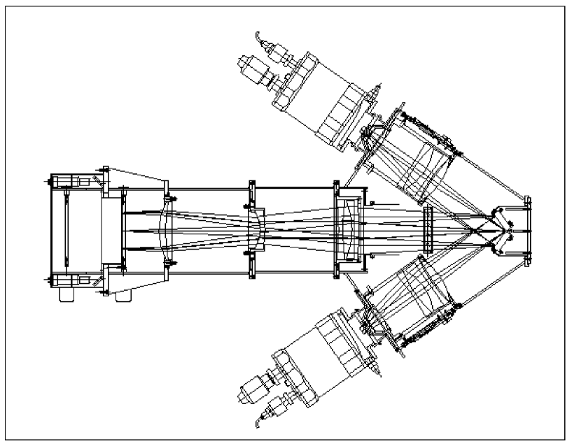
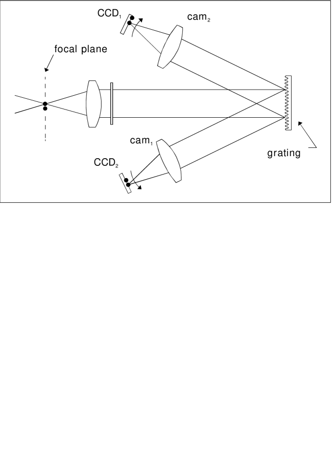
4.2 Optics

The optical system of the PN.S (see Fig. 4) consists of a collimator with 5 elements in 4 groups, the largest lens being 240 mm in diameter, a narrow-band filter, twin 600 l/mm gratings, and a pair of nominally identical cameras (6 elements in 5 groups) in which the largest element has 210 mm diameter. For ease of manufacture the design was restricted to spherical surfaces, despite the fact that the anamorphic reflection at the gratings (transforming a nominally square field into one with with an aspect ratio of 0.9) presented a significant challenge.

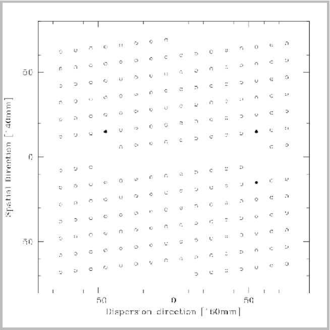
Table 3 lists the optical parameters of the instrument as built. The indicated operating range is nominal – chromatic effects are not severe and the instrument will function slightly outside this band, though the coatings will not be optimal. The computed imagery (Fig. 5) is valid over this range.

The gratings are standard items except that we requested 140 x 80 x 24 mm substrates replicated to the very edge, and bevelled at the grating input angle so as to facilitate butting with minimal ‘dead’ area. We required tight tolerance on the alignment of the grooves with the substrate edges so as to keep the dispersion directions in the two cameras parallel.

The grating input angle between the collimator axis and the grating normal is such that at a wavelength of 5010Å the centre of the field is centered on the CCD. The gratings are in principle at a fixed angle, and the detectors at a fixed position, so that as the wavelength is changed the centre of the field moves laterally across the chip. As the imaging quality of the spectrograph is rather closely matched to the size of the chip, it may be said that the usable field gradually “walks off” the detector. The “walkoff rate” is about the same as the dispersion, i.e. 17.4 µm per Å, or $\pm 1.04$ mm over the full operating range of the instrument ($\pm 60$Å). This is only 3.8% of the field, however, so although the grating tilts could be manually adjusted to recentre the image it is not anticipated that this will be done regularly.

Table 3: Final parameters of spectrograph optics.

Operating range	4950-5070Å
Grating(s)	Spectronic 35-53 600 8.5∘ blaze
Input angle (at grating)	26.6∘
Output angle (in first order)	8.4∘(on-axis at 5010Å)
I.A.	35.0∘
Collimator	F.L. = 1291 mm
Camera	F.L. = 287 mm
Image quality	EER   $\leq 18$ µm
Dispersion	0.0174 mm/Å

The design goal was for a total system efficiency of at least 30% at the WHT, about twice that of the general-purpose spectrograph (ISIS) at that telescope, with $\sim 5$ times larger field. The estimates in Table 4, based on the final optical design, published data and calculations, suggested that this was feasible.

Table 4: Estimated Optical Efficiencies.

Component	Efficiency	Basis of estimate
Grating	0.83	E.M. calculation assuming aluminium at 5010Å
Lenses	0.97	reflection loss (0.1% at 10, and 0.2% at 8 air/glass interfaces)
Lenses	0.95	bulk absorption, total path length 213 mm
Window	0.98	dewar window without special coating
PN.S total	0.73
Filter	0.80	manufacturer’s specifications
Detector	0.85/0.90	ING/TNG measurements
Telescope	0.72/0.63	observatory calculations for WHT Cassegrain/TNG Nasymyth
System	0.37/0.33	at WHT/TNG

Although the two telescopes for which the instrument has been designed (§4.1) are of similar diameter and have the same focal ratio, the optics are sufficiently different in detail that it was difficult to produce a single PN.S design for both. Full control of the aberrations appeared to require interchangeable optical elements, which introduced too much cost and complexity. We agreed on a single design in which the imaging quality is compromised, but not noticeably so under normal observing conditions (see Fig. 5).

Parameters which depend on the telescope are listed in Table 5. In this table a pixel size of 13.5 µm has been assumed, in agreement with the detectors used for commissioning. The images are slightly better sampled at the WHT owing to the longer focal length, but with this pixel size would still be adequately sampled at the TNG down to 0.7″ seeing. The field sizes indicated correspond to the projected extent of the 2048 x 2048 element detector currently in use. At both telescopes the unvignetted field is about 10′ square.

Table 5: Parameters of the PN.Spectrograph at Telescopes.

Telescope	4.2m WHT	3.5m TNG
Focal station	f/10.942 Cassegrain	f/10.755 Nasmyth
Diameter of pupil (at grating)	117.9 mm	120.0 mm
Scale (pxl/arcsec)
(in dispersed direction)	3.32	2.72
(in spatial direction)	3.67	3.01
Nominal field   (arcmin)	11.43 x 10.34	13.95 x 12.59

Figure 5: Spot diagrams for one arm of the spectrograph, at 5010Å. The left column shows the raytraced spot diagram for (from top to bottom) the WHT at field centre, the WHT in a corner of the field, the TNG at field centre, and the TNG in a corner of the field (the box is 60µm square) - note the very asymmetric spot pattern due to the half-pupil. Subsequent columns show the same spots convolved (from left to right) with gaussian seeing of 0.5, 0.7 and 1.0 arcsec, where the box size is now 120µm square and allowance has been made for the anamorphic ratio of 0.9, which compresses the images in the vertical (dispersion) direction.

Details of the optical design (ZEMAX files) “as built” can be obtained from the project website or on request to the team. In addition, optimised designs for the WHT and for the TNG are also available.

The V-type coatings on the camera optics (10 surfaces in each camera) were specified as having maximum reflectance of 0.1% within the operating range. For the collimator (8 surfaces) a W-type coating was specified with a maximum reflectance of 0.2% over the operating range and 0.3% over a secondary range covering 6488 - 6645Å. This was to allow the possibility of the addition of a H$\alpha$-camera (§7), and is also the reason that the [O III] filter has been placed “downstream” of the collimator. The manufacturer’s calculations for the residual reflection were consistent with these specifications for normal incidence.

The science goals of the instrument led us to an initial choice of narrow-band [O III] filters centred at around 5000Å, 5034Å and 5058Å. The FWHM of 31-35Å is deliberately small to minimize the background noise, and the filters are designed to be tiltable by up to 6^∘ so that they can be tuned to the systemic velocity of each target. Optical tolerances on the 195 mm diameter circular filters were held tight in order to achieve maximum homogeneity across the field and at large tilt angles. However, as the filters are rather near the pupil for the reason mentioned in the previous paragraph, there is significant shift in the bandpass over the field and this effect is amplified when the filters are tilted, setting limits on the usable field size in the direction of tilt.

For the 5034/31.4Å filter at 0^∘ incidence the shift in bandpass over the field reduces the useful bandpass, in the sense of unbiassed velocity coverage, to about 29.6Å. At 6^∘ incidence this quantity is reduced to 17.0Å, or 1000 km s^-1 in velocity. The bandpass becomes even smaller when the diagonals of the field are considered. Whether the reduced bandpass is acceptable depends on parameters of the object under study, most obviously its size.

4.3 Mechanical design

The mechanical design is in most respects straightforward, the main priority being rigidity. Stiffness is vital since relative displacement of the two images by a few microns causes tens of km s^-1 shift in velocity. Structural analysis predicts that the maximum flexure in either spectral or spatial directions should correspond to an image displacement of only about 0.02 pixel (0.01″ on sky) when the spectrograph is moved through the full range of positions encountered at either the Cassegrain or Nasmyth focus. This degree of rigidity is more than sufficient since small movements of the detector are likely to be considerably more significant.

Figure 6: Photograph of the unusual grating mount in which two identical gratings (but with blaze direction reversed) are oriented in a ‘concave’ arrangement.

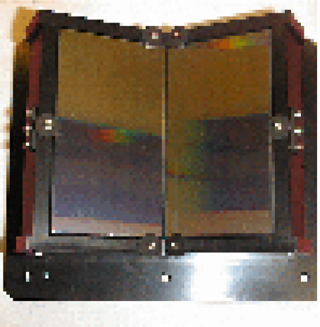
A second problem to be addressed was that of butting together the gratings. An earlier “convex” arrangement in which the gratings would be replicated on a prism-shaped substrate was rejected on the grounds that the fabrication was too critical: once constructed, no adjustment of the parallism of the two sets of grooves would have been possible, and of course the angle between the two grating normals would have been fixed also. In the “concave” arrangement chosen (Fig. 6) the butted edges are bevelled at the appropriate angle to minimise light loss at the join, and the two gratings held in place by the mount.

The spectrograph incorporates just two (d.c.) motors, one to move the calibration mask (Fig. 8) into the focal plane and one to drive a plate across the beam to serve as a shutter. Tilting of the [O III] filter has to be done by hand, after opening an access hatch. Tilting is achieved by rotating one wedged surface against another, facilitated by a tool on which the corresponding tilt angle is marked (Fig. 7). The operation requires the telescope (in the case of the WHT) to be parked at the zenith and takes about 5 minutes, including slewing. A complete filter change requires considerably more time and targets have so far been scheduled to avoid the neccessity of this being done during the night.

Figure 7: Photograph of the filter area, showing the tool used to tilt the filter by a calibrated amount by altering the alignment of two wedged surfaces.

4.4 Calibration

Figure 8: Focal plane calibration mask: 0.20 mm diameter holes in the metal mask are so arranged that the resulting spectra (dispersed horizontally) do not overlap (in order to determine the orientation of the images unambiguously three holes are 50% oversized). The large number of holes facilitates an over-constrained solution for the wavelength-dependent mapping of the focal plane onto the detector. Illumination with a spectral lamp will give rise to 2-4 points per hole, depending upon the filter in use. The single slit near the centre can be used when (e.g.) a stellar spectrum is necessary for an independent velocity calibration.

As discussed in the references in §3.5, calibration of CDI data requires taking account of the internal distortions, which are dominated by the approximately parabolic distortion resulting from the reflection at the grating (“slit curvature”), which is an additive effect when one compares counter-dispersed image pairs. Other, smaller, effects include the discrepancies in the position of objects in the two images as a result of the inevitable differences between the optics in the two cameras.

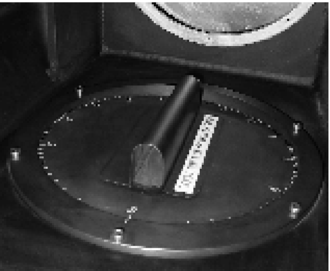
A map of all the distortion terms, including wavelength dependences, can be determined by the use of a calibration mask (Fig. 8) which can be placed in the focal plane. In combination with spectral line lamps (typically CuAr and CuNe) and continuum lamps a spectrum-dependent calibration over the whole field can be obtained. On-sky calibrations are only necessary to check photometry, though Galactic PN (with catalogued radial velocities) are regularly observed to cross-check procedures. Although we are still refining these procedures the velocity residuals are currently no greater than 28 km s^-1 (see §4.6).

The final step in the calibration is to obtain accurate astrometry for the newly-found PN. This is done by defining a cartesian coordinate system in which the positions of a number of foreground stars are defined by the coordinates about which the counter-dispersed spectra are symmetric. For example if the intensity-weighted average position of a stellar spectrum in one image is $(x_{L},y)$ and in the other $(x_{R},y)$, then $((x_{L}+x_{R})/2,y)$ can be taken as the stellar position. These positions are then compared with astrometric catalogues to obtain a plate solution in the usual way. The sky co-ordinates of the PN calculated on this basis will be correct, but the velocities will have an offset, in this example, corresponding to the intensity-weighted mean wavelength of the filter. But this offset does not need to be determined explicitly since the calibration mask fixes the absolute wavelength scale for each pair of PN detections.

4.5 Project overview

The PN.Spectrograph consortium, whose members are listed on the project website⁴ was formed in 1997. The project is funded by means of grants received from the national funding agencies of the participating institutes, and from ESO. Total expenditure up to the commissioning of the instrument was EUR 212k, which includes seven man-months of mechanical workshop effort provided directly by the Dutch astronomy foundation ASTRON. Academic labour and travel costs were not charged to the project. Also, CCD detectors and cryostats are not included in the budget. By prior agreement the spectrograph makes use of the observatory detectors and data management systems.

The optical design was contracted to Prime Optics (Australia) who worked closely with the workshops of the RSAA where the mechanical design was carried out. Contracts for the construction of the camera optics and the collimator optics went out to INAOE (Mexico) and to the RSAA optical workshop, respectively, in March 1999. Acceptance testing was carried out in May 2000 but this was inconclusive and the optics could not be accepted until December, following further tests and corrective work by RSAA. The optics were then coated by the Australian company Rofin during February-March 2001.

In the meantime a Phase B study, to identify any remaining problems such as stray light and flexure, had been carried out by RSAA and project members. Completed in July 1999, it showed that a double specular reflection (zeroth order) between the gratings (which ‘face’ each other in the concave arrangement chosen - see Fig. 4) would give rise to a significant ghost image. This problem was solved by chosing different gratings, which were then ordered from the Richardson Grating Laboratory.

ASTRON constructed the instrument housing and many of the component mountings, which were shipped to Australia in July 2000 for assembly. The first of the filters, from BARR associates, arrived in mid-May.

The RSAA workshops also manufactured the adapter flange for the WHT Cassegrain (a different one is required for the TNG), the adapters for the WHT cryostats, the tilt-tunable filter holder, the grating assembly and the two motorized units (shutter and calibration mask). Finally, the RSAA was contracted to correct any residual mechanical errors, and to integrate and align the instrument.

During final testing, conducted by RSAA and Prime Optics staff, a subtle scattered-light problem appeared which had not been identified during the Phase B study. It again involved multiple reflections from the grating assembly and appeared when the (small) reflectance of the CCD detectors was included. The problem was solved by an additional baffle.

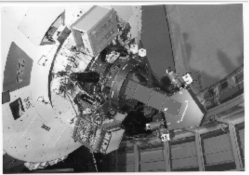
4.6 The PN.S in operation

The instrument was shipped to La Palma in the Canary Islands in June 2001, but unfortunately misdirected to Las Palmas, before arriving at the Observatory on July 10. The PN.S was commissioned at the 4.2m WHT of the ING on July 16, 2001 (Merrifield et al., 2001). It was then operated for a further three nights and has since been used in two observing runs (September 2001 and March 2002). All observations were made with the EEV-12 and EEV-13 detectors, and to date only the 5034Å filter has been used, at either 0^∘ tilt ($\lambda_{c}$ = 5034.3) or 6^∘ tilt ($\lambda_{c}$ = 5027.1).

Figure 9: The PN.Spectrograph at the WHT.

From measurements of galactic PN with catalogued fluxes and of spectrophotometric standard stars we were able to determine the system efficiency (corrected for atmospheric losses) to be 33.3%, in good agreement with the design expectations (Table 4). Here the “system efficiency” includes telescope, instrument including filter, and detector, and represents the throughput at the peak of the filter profile. Since the dispersion has been determined, it is easy to establish the peak throughput per Ångstrom by measuring the flux in a slice through the peak of the spectrum of a standard star and comparing this with the expected flux.

To use this information to establish a magnitude limit, we refer to §2 from which we can see that at the distance of the Virgo cluster (15 Mpc) the brightest PN have $m^{*}\sim 26.6$. At the above efficiency, in a one-hour observation with 1″ seeing, this corresponds to about 1200 detected photons and a S/N of about 10.1 in each arm of the spectrograph, using Equation 7. PN which are 1.4 magnitudes fainter reach $S/N\sim 10$ in 12.0 hours. Even at a distance of 25 Mpc ($m^{*}\sim 27.7$), significant sampling of the PNLF can be achieved ($S/N\sim 7$ for $m^{*}+0.6$ mag in 14.6 hours).

Preliminary measurements show a differential displacement between the left and right images of up to 3 pixels ($\sim 40$µm) when the telescope is rapidly slewed through the full range of azimuth and elevation, which is much more than that expected from flexure calculations (§4.3). Most of this effect seems to be due to residual movements of the CCD detectors within the cryostats, which was not included in the calculation.

Fortunately, by taking arc lamp images of the focal plane mask at regular intervals during observations, we are able to ensure that the velocity calibration is not affected by flexure. After slewing to each new target the zero point of the flexure is determined by registration of the calibration mask in the two cameras. Measurements have also shown that the displacements in either image are negligibly small during normal guiding ($\pm 0.5$ pixel r.m.s.) so the imaging is not compromised.

The wavelength calibration, still being optimised, has tested out quite satisfactorily during observations of objects with known velocities. For example, a comparison of 25 of our measured PN velocities in NGC 3379 ($D$ = 10 Mpc) with measurements from the NESSIE multi-fibre spectrograph on the KPNO 4-m telescope (Ciardullo et al., 1993) shows good agreement, indicating our measurement uncertainty at this stage to be 28 km s^-1 (Fig. 10).

Figure 10: Velocities of 25 planetary nebulae in NGC 3379, as measured with the PN.S and NESSIE. The solid line indicates a perfect correspondence, and the dotted lines show uncertainty boundaries of $\pm$ 28 km s^-1 for the PN.S. The error bars show the NESSIE measurement uncertainties of 7 km s^-1.

For conditions under which the seeing was worse than $\sim 0.8$″ the image quality was uniform over the field. Under better conditions, it becomes evident that the image quality is slightly poorer towards the corners of the field, as expected (see Fig. 5). Under very good conditions the imaging quality is limited by the spectrograph optics to $\sim 0.7$″.

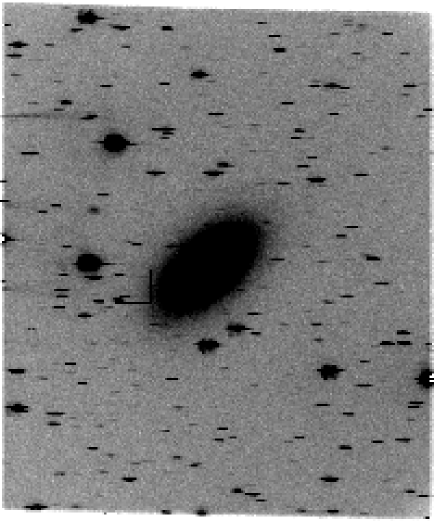
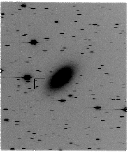
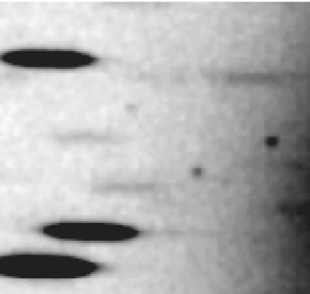
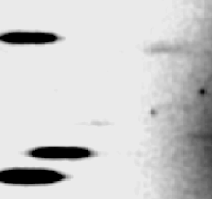
Images from one of the first observing sessions at the WHT are shown in Fig. 11. The left- and right-arm images appear nearly identical, since they are visually dominated by the short, symmetric spectra of stars and by the broad, integrated light of the galaxy (NGC 7457). However the positions of the PN, some of which can be seen as point-like sources in the zoomed-in images, are displaced between left and right images, as can be seen by comparing them with the stellar features (cf Fig. 2).

Figure 11: Images of NGC 7457 taken with the PN.S in September 2001. The CDI pair is shown at the top; the lower panels show detail in the boxed region, showing stellar ‘images’ and the displaced positions of PN.

5 Conclusion

We have constructed an instrument which can efficiently detect extragalactic PN and measure their velocities. Using a novel application of slitless spectroscopy, the data can be obtained in a single observation with a single instrument, rather than the more complex procedures previously necessary. We have presented design information for the highly optimised, dedicated instrument now in use at La Palma, and first results have been presented. In effect the telescope efficiency can be nearly doubled by this approach, opening up the prospect of routine observations of galaxy kinematics at a distance of up to 25 Mpc with 4m-class telescopes. The technique is applicable to larger telescopes.

6 Acknowledgements

The PN.S would not have seen the green light of day without the generous financial support of: the Australian Research Council, the European Southern Observatory, the Italian C.N.A.A. (Consiglio Nazionale per l’Astronomia e l’Astrofisica), the Dutch N.W.O. (Nederlandse Organisatie voor Wetenschappelijk Onderzoek), the Observatory of Capodimonte and in Britain the Royal Society and PPARC.

We thank the ING (operating the William Herschel Telescope on La Palma) for their enthusiastic support, the Mt Stromlo workshops of the R.S.S.A. for their untiring efforts, and the Anglo-Australian Observatory. We also wish to thank Steve Rawlings, who generously assisted by swapping his telescope time allocation after delays caused planning problems for the project, and Rob Hammerschlag and and Felix Bettonvil for technical advice.

7 Appendix A: Undispersed H$\alpha$ arm

An H$\alpha$ imaging camera was included as a future option in the PN.S design. A dichroic can be placed after the last element of the collimator, bringing an undispersed image to a third CCD detector via a H$\alpha$ filter and camera. We are now seeking to fund this option. The motivation is to improve the detection efficiency of PN and to permit deep Halpha imaging of galaxies which we are already surveying for PN.

For those PN which are detected in H$\alpha$, the H$\alpha$ image constitute a cross-check of the velocity measurement. The image will also serve as a check on the astrometric procedures used on the CDI images, and as an indicator of contaminating objects. For example, the absence of an H$\alpha$ counterpart to an [O III] detection will indicate a background object instead of a PN: Ly-$\alpha$ emitters redshifted to the [O III] band are detected in significant numbers in [O III] surveys (e.g. Freeman et al. (2000)). Objects which are relatively bright in H$\alpha$ may be unresolved HII regions. Although the [N II] $\lambda 6584$Å line will often be included in the H$\alpha$ image, some information on the H$\alpha$/[O III] ratio would be obtained.

While elliptical galaxies harbour much less cold and warm gas than spirals, with deep enough exposures they mostly show extended H$\alpha$ emission (Macchetto et al., 1996)). With our long integration times (typically 10 hours on each galaxy, and with an optical efficiency higher than that obtained with multi-purpose instruments), we expect to achieve some of the deepest H$\alpha$ images yet (for example, about a factor of 6 deeper than the images of Macchetto et al. (op. cit.) in their survey at the ESO 3.6m and 3.5m NTT). These new emission maps may provide useful insight into the ionization processes in elliptical galaxies. Similar deep H$\alpha$ images can be acquired in the outer regions of S0 galaxies, where any remaining interstellar gas is probably ionized by the intergalactic UV radiation. Long integration times are required to detect this diffuse ionized gas (see Bland-Hawthorn et al. (1997)), which may help to constrain the ionizing flux and gas density (Maloney and Bland-Hawthorn, 1999).

8 Appendix B: Rejected design solutions

Several other possibilities exist for the construction of a simultaneous CDI instrument such as the PN.S. For future reference we briefly summarise some that we have investigated.

8.1 Amplitude splitting

Figure 12: Amplitude splitting of the wavefront.

Instead of a pair of gratings butted together (pupil splitting) we consider a single grating illuminated at normal incidence (Fig. 12). By choice of grating constant, only the orders $m=$ -1, 0 and 1 are propagating. Therefore, the only possible source of stray light is from the $m=0$ order, which in this case would not be a great problem. This is an elegant construction since symmetry is guaranteed, there is no join between the two gratings, and the mechanical mounting is trivial.

Connes (1959) explored this approach in various interferometer designs, and believed on the grounds of a scalar analysis that a grating with a suitable symmetric triangular profile would split light at normal incidence into two beams with nearly 50% efficiency in each. Using electromagnetic code we discovered that for a 1800l/mm grating the optimum efficiency (averaged over both polarisations) is only 64% (in aluminium) at a blaze angle of 34^∘, slightly displaced with respect to the 32^∘ expected on the basis of geometric. This is well short of the nearly 100% optical efficiency expected by Connes, and the difficulty of construction does not justify its use when compared with a holographically produced grating. Incidentally Connes’ expectation does work out correctly for the S-polarised component.

We performed an efficiency optimisation for a holographic grating, assuming a sinusoidal profile again in aluminium. A regime of high ($>80$%) efficiency is found near 1250l/mm and a groove depth of 0.165 µm (the p- and s-polarisation efficiencies are about equal). The cost of a custom-made grating would have been prohibitive though, while the highest efficiency for an industry standard holographic grating was found to be around 66% in unpolarised light, with 1800l/mm and a groove depth of 0.16 µm.

8.2 Polarization splitting

The problem of obtaining high efficiency from a grating is made much easier if the grating is illuminated by light of only one polarization. A CDI instrument arises if the light is split into two linearly-polarized beams, each of which is fed to a separate grating Fig. 13). The idea calls for a more complicated mechanical design though, and the resulting asymmetries were feared to lead to flexure problems.

Figure 13: CDI using polarisation splitting. The unpolarised light is divided into two beams by means of a polarising beamsplitter (see view B, in which the reflected beam also traverses a compensation plate). The reflected light (view C, looking down from the telescope axis) and the transmitted light (view A) encounter similar, but polarisation-optimised, spectrographs.

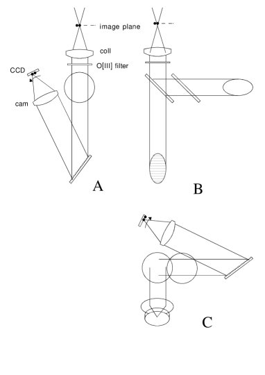
8.3 Transmissive gratings

The transmissive equivalent of pupil splitting would correspond to two grisms, side-by-side. This would make it possible to use one camera instead of two, the two images falling side-by-side on a single large format CCD. During our study we were unable to find a grism with sufficient dispersion and efficiency.

We did investigate the idea of a transmissive phase mask, in which the collimated beam is passed through a crenellated dielectric structure which causes it to diffract into pairs of orders (similar to the case in §8.1). Provided the zeroth order is minimised by selecting the groove depth, and higher orders are cut off, high efficiency can be achieved in the –1 and +1 orders. A review is given by Walker et al. (1993), who show the effect of varying all parameters including the duty cycle of the structure, indicating that high efficiency can be obtained.

In an early (1994) scaled experiment using a microlithographically produced mask and UV light, we verified that high transmitted efficiencies ($\sim 75$%) can be reached At the time, it was difficult to obtain these structures in large sizes. Since then, the closely related VPH (volume phase holographic) gratings have become available, and transmissive gratings may be a more viable option.

9 Appendix C: Accuracy of PSF-fitting photometry and positions

Here we calculate the accuracy of object centroids derived by means of PSF fitting.

Let $f_{i}$ be the data: intensities on the pixels $i$ at positions $x_{i},y_{i}$ (in units of pixels) on the image plane. We try to model these data as $AP(x_{i}-\mu_{x},y_{i}-\mu_{y})\Delta^{2}$, where $\Delta$ is the pixel width, and $P$ is the PSF normalized to total intensity 1. $A$ is the intensity of the star, and $(\mu_{x},\mu_{y})$ are the position of the star, to be fitted for. Write

$$\chi^{2}=\sum_{i}\left(f_{i}-AP(x_{i}-\mu_{x},y_{i}-\mu_{y})\Delta^{2}\right)^{2}/\sigma_{i}^{2}$$

where $\sigma_{i}$ is the error on the measured intensity in pixel $i$. Then the minimum of $\chi^{2}$ gives the best-fit PSF, and the second partial derivatives of $\chi^{2}$ with respect to any two parameters give twice the inverse covariance matrix. In what follows we ignore covariances between the different variables $A$, $\mu_{x}$ and $\mu_{y}$, as is appropriate for bisymmetric PSF’s.

At the best-fit value (we may assume without loss of generality that $\mu_{x}=\mu_{y}=0$) we obtain the inverse variance on the star’s intensity $A$ as

$$\hbox{Var}(A)^{-1}=0.5\ \partial^{2}\chi^{2}/\partial A^{2}=\sum_{i}P(x_{i},y_{i})^{2}\Delta^{4}/\sigma_{i}^{2}$$

which reduces to

$$=\left(\int\int P^{2}\ dxdy\right)\Delta^{2}/\sigma^{2}$$

if the PSF is fully sampled and $\sigma_{i}$ constant (i.e., background-limited data). All integrals are over the range $0-\infty$.

The inverse variance of the best-fit position is similarly (removing terms which go to zero at the best fit)

$$\hbox{Var}(\mu_{x})^{-1}=0.5\ \partial^{2}\chi^{2}/\partial\mu_{x}^{2}=\sum_{i}A^{2}(\partial P/\partial x)^{2}\Delta^{4}/\sigma^{2}=\left(\int\int(\partial P/\partial x)^{2}dx\ dy\right)A^{2}\Delta^{2}/\sigma^{2}$$

(and similarly for $\mu_{y}$). These two relations can be combined to give

$$\delta\mu_{x}={\delta A\over A}\times\sqrt{\int\int P^{2}\ dxdy\over\int\int(\partial P/\partial x)^{2}\ dxdy}$$

where $\delta A=\hbox{Var}(A)^{1/2}$ is the 1-$\sigma$ error on $A$, etc.

The centroid error therefore depends on the significance $A/\delta A$ of the detection of the star, and on a geometric factor governed only by the shape of the PSF.

For a gaussian PSF, dispersion $s$, we find

$$\hbox{Var}(A)^{-1}=\Delta^{2}/(4\pi s^{2}\sigma^{2})$$

hence

$$\delta A=\sqrt{4\pi}s\sigma/\Delta$$

and

$$\hbox{Var}(\mu_{x})^{-1}=A^{2}\Delta^{2}/(8\pi s^{4}\sigma^{2})$$

hence

$$\delta\mu_{x}=\sqrt{8\pi}s^{2}\sigma/(\Delta A)=\sqrt{2}s{\delta A\over A}$$

For a Moffat function PSF of the form

$$P={\beta-1\over\pi a^{2}}\left(1+{r^{2}\over a^{2}}\right)^{-\beta}$$

we get

$$\delta\mu_{x}=a{\delta A\over A}\sqrt{2\beta+1\over\beta(2\beta-1)}$$

If we write $a$ as $\frac{1}{2}\hbox{FWHM}/\sqrt{2^{1/\beta}-1}$, we find that for $\beta>1.5$, which covers PSF’s with tails as shallow as $r^{-3}$

$$\delta\mu_{x}={\delta A\over A}\times 0.67\times\hbox{FWHM}\pm 10\%.$$

(The gaussian is the limit $\beta\to\infty$; in this case the coefficient is 0.6.)

References

- Arnaboldi et al. (1996) Arnaboldi, M., Freeman, K.C., Méndez, R.H., Capaccioli, M., Ciardullo, R., Ford, H., Gerhard, O., Hui, X., Jacoby, G.H., Kudritzki, R.P., and Quinn, P.J. 1996, ApJ, 472, 145
- Arnaboldi et al. (1998) Arnaboldi, M., Freeman, K.C., Gerhard, O., Matthias, M., Kudritzki, R.P., Méndez, R.H., Capaccioli, M., and Ford, H. 1998, ApJ 507, 759
- Arnaboldi et al. (2002) Arnaboldi, Magda, Aguerri, J. Alfonso L., Napolitano, N.R., Gerhard, O., Freeman, K.C. Feldmeier, J., Capaccioli, M., Kudritzki, R.P., and Méndez, R.H. 2002, AJ, 123, 760
- Bland-Hawthorn et al. (1997) Bland-Hawthorn, J., Freeman, K, and Quinn, P. 1997, ApJ, 490, 143
- Ciardullo (1987) Ciardullo, R., Ford, H.C., Neill, J.D., Jacoby, G.H., and Shafter, A. W. 1987, ApJ, 318, 520
- Ciardullo et al. (1989) Ciardullo R., Jacoby G.H., Ford H.C., and Neill J.D. 1989, ApJ, 339, 53
- Ciardullo et al. (1991) Ciardullo, R., Jacoby, G.H., and Harris, W.E. 1991, ApJ, 383, 487
- Ciardullo et al. (1993) Ciardullo, R., Jacoby, G.H., and Dejonghe, H.B. 1993, ApJ, 414, 454
- Ciardullo (1995) Ciardullo, R. 1995, in Highlights of Astronomy, ed. I. Appenzeller, 10, 507
- Ciardullo et al. (2002a) Ciardullo, R., Feldmeier, J.J., Jacoby, G.H., Kuzio, R.E., Laychak, M.B., and Durrell, P.R. 2002, ApJ(submitted)
- Ciardullo et al. (2002b) Ciardullo, R., Feldmeier, J.J., Krelove, K., Jacoby, G.H. and Gronwall, C. 2002, ApJ, 566, 784
- Connes (1959) Connes, P. 1959, Revue D’Optique, 38, no4, 157
- Dopita et al. (1992) Dopita, M.A., Jacoby, G.H., and Vassiliadis, E. 1992, ApJ, 389, 27
- Douglas and Taylor (1999) Douglas, N.G., and Taylor, K. 1999, MNRAS, 307, 190
- Douglas et al. (2000) Douglas, N.G., Gerssen, J., Kuijken, K., and Merrifield, M. 2000, MNRAS, 316, 795
- Fehrenbach (1947) Fehrenbach, C. 1947, Annales D’Astrophysique, 10, 306; see also subsequent papers 10, 257 and 11, 35.
- Feldmeier et al. (1997) Feldmeier, J.J., Ciardullo, R., and Jacoby, G.H. 1997, ApJ, 479, 231
- Ferrarese et al. (2000) Ferrarese, L., Ford, H.C., Huchra, J., Kennicutt, R.C., Mould, J.R., Sakai, S., Freedman, W.L., Stetson, P.B., Madore, B.F., Gibson, B.K., Graham, J.A., Hughes, S.M., Illingworth, G.D., Kelson, D.D., Macri, L., Sebo, K., and Silbermann, N.A. 2000, ApJS, 128, 431
- Freeman et al. (2000) Freeman, K.C., Arnaboldi, M., Capaccioli, M., Ciardullo, R., Feldmeier, J., Ford, H., Gerhard, O., Kudritzki, R.P., Jacoby, G., Méndez, R.H., and Sharples, R. 2000, ASP Conference Series 197, 389
- Geyer and Nelles (1985) Gelles, E.H., and Nelles, B. 1985, A&A, 148, 312
- Hui (1993a) Hui, X. 1993a, PASP, 105, 1011
- Hui et al. (1993b) Hui, X., Ford, H.C., Ciardullo, R., and Jacoby, G.H., 1993b, ApJ, 414, 463
- Hui et al. (1995) Hui, X., Ford, H.C., Freeman, K.C., and Dopita, M.A. 1995, ApJ, 449, 592
- Jacoby et al. (1990) Jacoby, G.H., and Ciardullo, R., Ford, H.C. 1990, ApJ, 356, 332
- Kudritzki et al. (2000) Kudritzki, R.-P., Méndez, R. H., Feldmeier, J. J., Ciardullo, R., Jacoby, G. H., Freeman, K. C., Arnaboldi, M., Capaccioli, M., Gerhard, O., and Ford, H. C. 2000, ApJ, 536, 19
- Macchetto et al. (1996) Macchetto, F., Pastoriza, M., Caon, N., Sparks, W. B., Giavalisco, M., Bender, R., and Capaccioli, M. 1996, A&AS, 120, 463
- Maloney (1993) Maloney, P. 1993, ApJ, 414, 41-56
- Maloney and Bland-Hawthorn (1999) Maloney, P., and Bland-Hawthorn, J. 1999, ApJ, 522, L81
- Maystre (1978) Maystre, D. 1978 J. Opt. Soc. Am., 68, 490
- Méndez et al. (2001) Méndez, R.H., Riffeser, A., Kudritzki, R.-P., Matthias, M., Freeman, K. C., Arnaboldi, M., Capaccioli, M., and Gerhard, O. E. 2001, ApJ, 563, 135
- Merrifield et al. (2001) Merrifield, R., Douglas N.G., Kuijken, K., and Romanowsky A. 2001, ING Newsletter 5, 17
- Merritt (1997) Merritt, D. 1997, AJ, 114, 1074
- Merritt and Saha (1993) Merritt, D., and Saha, P. 1993, ApJ, 409, 75
- Merritt and Tremblay (1993) Merritt, D., and Tremblay, B. 1993, AJ, 106, 2229
- Napolitano et al. (2001) Napolitano, N. R., Arnaboldi, M., Freeman, K. C., and Capaccioli, M. 2001, A&A, 377, 784
- Naylor (1998) Naylor, T. 1998, MNRAS, 296, 339
- Romanowsky and Kochanek (2001) Romanowsky A.J, Kochanek C.S. 2001, ApJ, 553, 722
- Saglia et al. (2000) Saglia, R.P., Kronawitter, A., Gerhard, O., and Bender, R. 2000, AJ, 119, 153
- Tremblay et al. (1995) Tremblay, B., Merrit, D., and Williams, T.B. 1995, ApJ, 443, L5
- Walker et al. (1993) Walker, S.J, Jahns, J., Li L., Mansfield, W.M., Mulgrew, P., Tennant, D.M., Roberts, C.W., West, L., and Ailawadi, N.K. 1993, Applied Optics, 32, 2494