NONLINEAR EFFECTS IN MODELS OF THE GALAXY:
1. MIDPLANE STELLAR ORBITS IN THE PRESENCE OF 3D SPIRAL ARMS

Abstract

With the aim of studying the nonlinear stellar and gaseous response to the gravitational potential of a galaxy such as the Milky Way, we have modeled 3D galactic spiral arms as a superposition of inhomogeneous oblate spheroids and added their contribution to an axisymmetric model of the Galactic mass distribution. Three spiral loci are proposed here, based in different sets of observations. A comparison of our model with a tight-winding approximation shows that the self-gravitation of the whole spiral pattern is important in the middle and outer galactic regions. A preliminary self-consistency analysis taking ${\Omega}_{p}$ = 15 and 20 km s^-1 kpc^-1 for the angular speed of the spiral pattern, seems to favor the value ${\Omega}_{p}$ = 20 km s^-1 kpc^-1. As a first step to full 3D calculations the model is suitable for, we have explored the stellar orbital structure in the midplane of the Galaxy. We present the standard analysis in the pattern rotating frame, and complement this analysis with orbital information from the Galactic inertial frame. Prograde and retrograde orbits are defined unambiguously in the inertial frame, then labeled as such in the Poincaré diagrams of the non-inertial frame. In this manner we found a sharp separatrix between the two classes of orbits. Chaos is restricted to the prograde orbits, and its onset occurs for the higher spiral perturbation considered plausible in our Galaxy. An unrealistically high spiral perturbation tends to destroy the separatrix and make chaos pervasive. This may be relevant in other spiral galaxies.

1 INTRODUCTION

Modeling of spiral galaxies with sophisticated computational techniques has become the usual way to study systems of this nature. One of the important structures, which is in fact the one that gives the name to this type of galaxies, is the spiral pattern. In the spiral density wave theory (Lin & Shu 1964), the spiral structure of galaxies was modeled as a periodic perturbation term to the axisymmetric potential in the disk plane. This is known as the tight-winding or WKB approximation (e.g., Binney & Tremaine 1994) for small pitch angles. In the case of a two-armed spiral pattern it gives a potential in the galactic plane of the form:

$$\Phi_{s}(R,\varphi)=f(R)cos[2\varphi+g(R)];$$ (1)

The function $f(R)$ is the amplitude of the perturbation, $g(R)$ provides the geometry of the spiral pattern, and $R$, $\varphi$ are cylindrical coordinates in the non-inertial reference frame of the arms (rotating with a given angular velocity).

All studies of spiral galaxies we know of, even in cases of large pitch angle in the spiral pattern, have used a spiral potential of the form in Eq. (1), e.g. Contopoulos & Grosbøl (1986, 1988; hereafter C&G86 and C&G88); Patsis, Contopoulos, & Grosbøl (1991, hereafter PC&G), and in particular in our Galaxy the models of Amaral & Lépine (1997, hereafter A&L) and Lépine, Mishurov, & Dedikov (2001). Self-consistency of the proposed spiral pattern has been analyzed by C&G86, C&G88, PC&G, and A&L.

The dependence of the spiral potential on $z$ (perpendicular distance to the galactic plane) has been accounted for by Patsis & Grosbøl (1996) as a $sech^{2}(z/z_{s})$ factor of a function of the form in Eq. (1), with $z_{s}$ a scaleheight. Martos & Cox (1998), in numerical MHD simulations, considered an exponential z-factor of an approximate local spiral potential in the galactic plane.

In barred galaxies the approach is analogous to that given above for spiral galaxies: the usual approximation for the potential in the galactic plane due to the bar is a function of the form $\Phi_{b}(R,\varphi)=f(R)cos(2\varphi)$. Instead of taking an ad hoc dependence on the z coordinate, an alternative way to consider the extension to a 3D-bar potential is to begin directly with a 3D mass distribution representing the bar. This method has been considered by Athanassoula et al. (1983) and Pfenniger (1984). From a comparison on the galactic plane between their 3D-bar potential and a potential of the form $\Phi_{b}(R,\varphi)=f(R)cos(2\varphi)$, Athanassoula et al. (1983) found important differences in the corresponding force fields. However, the consequences of this result were not pursued.

In this paper, rather than using a simple ad hoc model for a 3D spiral perturbation, we consider a procedure whose essence is exactly the same as the modeling of a barred galaxy made by Athanassoula et al. (1983): instead of using a spiral potential of the form given by Eq. (1), we propose a 3D mass distribution for the spiral arms and derive their gravitational potential and force fields from previously known results in potential theory. Grand design galaxies with a very prominent spiral structure in red light suggest to us that such structure should be considered an important galactic component and are worthy of a modeling effort beyond a simple perturbing term. This approach amounts to little more than admitting the possibility that there is no simple formula that fits the spiral perturbation at all $R$.

In our model we use Schmidt’s (1956) analytical expression for the potential of an inhomogeneous oblate spheroid and model the spiral mass distribution as a series of such components settled along a spiral locus. The overlapping of spheroids allows a smooth distribution, resulting in a continuous function for the gravitational force. The basic parameters of the excess density distribution contributing to the spiral perturbation include a description of the spiral locus, the dimensions and density law of the spheroids, the central density in the spheroids as a function of galactocentric distance, the total mass of the spiral arms, and the angular velocity of the spiral pattern.

Our aim in this work is to make a preliminary study of stellar orbits in the Galactic plane $z$ = 0 in a potential resulting from the superposition of our 3D-spiral mass distribution and the axisymmetric Galactic mass distribution considered by Allen & Santillán (1991, hereafter A&S). Also, we compare the potential and force fields produced by the 3D-spiral mass distribution with a tight-winding approximation in Eq. (1). The resulting differences may have important consequences on the stellar and gaseous dynamical behavior in a potential of this type. An expected difference in the force field is the effect of the self-gravitation of the mass of the spiral arms, which is not accounted for in a potential like that of Eq. (1).

Detailed orbital studies have been made in barred and spiral galaxies (e.g. Contopoulos 1983, Athanassoula et al. 1983, Pfenniger 1984, Teuben & Sanders 1985). In this work our analysis of stellar motion in the Galactic plane, under the proposed Galactic potential, follows the usual technique of Poincaré diagrams. However, we propose an alternative interpretation of Poincaré diagrams which has not been previously considered. This interpretation is based on defining the orbital sense of motion (prograde or retrograde) in the Galactic inertial reference frame, joined to the usual definition in the non-inertial reference frame (e.g. Athanassoula et al. 1983) in which the spiral arms (and/or a bar) are at rest. This leads to Poincaré diagrams (meaningful only in the non-inertial reference frame) revealing two sharply separated regions: one corresponding to prograde orbits and the other to retrograde orbits. Our orbital analysis emphasizes the properties of the Galactic spiral arms for which some orbits may show stochastic behavior. These properties and the resulting stellar behavior should be applicable to similar types of galaxies.

The structure of this paper is the following: in Section 2 we present our Galactic model for the 3D spiral arms, with a discussion of the required parameters. In Section 3 we give the preliminary self-consistency tests that we have made of the proposed spiral arms, and establish a line of attack that must be followed to improve the model. In section 4 we make a comparison between the potential and force fields given by our model and those given by a tight-winding approximation. We show the importance of the self-gravitation of the spiral arms. In Section 5 we present an orbital analysis on the Galactic plane for differing spiral arms properties including the total mass in the spiral arms, the number of arms, and the angular velocity of the spiral pattern. In Section 5.1 we clarify the distinction between prograde and retrograde motion and the importance of the frame of reference to establish the essential difference between the two classes of orbits in Poincaré diagrams through the zero angular momentum separatrix, a concept we introduce in this section. We show here that our definition provides a direct connection between sense of orbital motion and chaotic motion. In the same subsection, Poincaré diagrams for a number of families labeled by their Jacobi integral $E_{J}$ are shown. An estimation of the required strength of the spiral perturbation for which the nonlinear effects are important is given, and we discuss the range of parameters explored and those we deem plausible for our Galaxy. In Section 5.2 we investigate the onset of chaos using Lyapunov exponents, and the comparison of resonances for prograde and retrograde motion. In Section 6 we discuss our results and give some conclusions, including the possible response of the interstellar gas to the Galactic potential.

2 THE MODEL

We use a Galactic model consisting of two mass distributions: the A&S axisymmetric model, and a 3D spiral model given by a superposition of oblate inhomogeneous spheroids along a given locus. The A&S Galactic model assembles a bulge and a flattened disk proposed by Miyamoto & Nagai (1975), with a massive spherical halo extending to a radius of 100 kpc. The model is mathematically simple, with closed expressions for the potential and continuous derivatives, which makes it particularly suitable for numerical work. The model satisfies quite well observational constraints such as the Galactic rotation curve and the perpendicular force at the solar circle. The main adopted parameters are $R_{0}=8.5$ kpc as the Sun’s galactocentric distance, and $V_{0}(R_{0})=220$ km s^-1 as the circular velocity at the Sun’s position. The total mass is $9\times 10^{11}M_{\odot}$, and the local escape velocity is 536 km s^-1. The local total mass density is $\rho_{0}=0.15M_{\odot}$ pc^-3. The resulting values for Oort’s constants are $A=12.95$ km s^-1 kpc^-1 and $B=-12.93$ km s^-1 kpc^-1.

As a first step to model the spiral mass distribution, we need the spiral locus. The optical spiral structure in our Galaxy has been studied by means of luminous HII regions (e.g, Georgelin & Georgelin 1976, Caswell & Haynes 1987). In the solar neighborhood the local inclination (pitch angle) of this spiral pattern has been inferred from the direction of the magnetic field lines (Heiles 1996), assumed to be aligned with the spiral arms (see reviews by Beck 1993, and Heiles 1995, on magnetic fields in spiral galaxies). In a recent study, Drimmel (2000) presents evidence for a two-armed spiral in our Galaxy as observed in the K band, which is associated with a non-axisymmetric component in the old stellar population. Figure 1 reproduces Fig. 2 of Drimmel (2000); the black squares trace the position of the four optical arms, and the open squares represent his 15.5^∘ pitch-angle fit for the two arms in the K band. The continuous line shows the first of three spiral loci we considered to model the spiral arms. These loci are obtained with a function $g(R)$ (see Eq. 1) of the form given by Roberts, Huntley & van Albada (1979),

$$g(R)=-(\frac{2}{N\ {\rm tan}\ i_{p}})\ {\rm ln}\ [1+(R/R_{s})^{N}]$$ (2)

with $i_{p}$ the pitch angle at $R$ $\rightarrow\infty$. In Figure 1 we take N=100, thus making the arms start at a distance $R_{s}$ and at right angles to a line passing through the Galactic center, $i_{p}$=11^∘, $R_{s}$=3.3 kpc, and we consider an orientation such that the two arms start on a line making an angle of 20^∘ with the Sun-Galactic center line (this is the approximate direction of the Galactic bar, e.g. Freudenreich 1998). This first two-armed spiral locus approximates the position of both optical and K-band arms.

As a second spiral locus, we take the two-armed, K-band locus itself. In Figure 2 the black and open squares give the K-band arms in Figure 1. The continuous line is obtained with the function $g(R)$ in Eq. (2), taking N = 100, $i_{p}$ = 15.5^∘, and $R_{s}$ = 2.6 kpc. We consider the effective starting distance of the spiral arms in this second locus as the distance 3.3 kpc taken in the first locus; the inner black squares in Figure 2 mark this position.

An important spiral locus is the one given by the four optical arms. Vallée (2002) shows in his Fig. 2 his fit to these optical arms, taking a pitch angle of 12^∘ and $R_{0}$ = 7.2 kpc for the Sun’s galactocentric distance. Figure 3 shows our fit with N = 100, $i_{p}$ = 12^∘, and $R_{s}$ = 3.54 kpc in Eq. (2), and $R_{0}$ = 8.5 kpc. Drimmel (2000) has suggested that the four optical arms in our Galaxy trace the response of the gas to the two-armed, K-band, stellar spiral arms in Figure 2. Thus, we take the third spiral locus for the spiral arms in our Galaxy as the superposition of the two-armed, K-band and four-armed, optical spiral loci. Galactic models using a superposition of two- and four-armed spirals have been proposed by A&L and Lépine, Mishurov, & Dedikov (2001).

Our set of models for the spiral mass distribution consist of a superposition of oblate inhomogeneous spheroids along each of the three proposed spiral loci. The minor axis of each spheroid is perpendicular to the Galactic plane. Each spheroid has a similar mass distribution, i.e., surfaces of equal density are concentric spheroids of constant semi-axis ratio. We consider a linear density law $\rho(a)=p_{0}+p_{1}a$ in the spheroids, with $a$ the major semi-axis of a similar surface, and the coefficients $p_{0}$, $p_{1}$ being functions of the galactocentric distance of the spheroid’s center. Schmidt (1956) has given the expressions for the potential and force fields for a spheroid with this density law.

With respect to the dimensions of the spheroids, Kennicutt & Hodge (1982) have analyzed a sample of spiral galaxies; from their Fig. 4, the average width of the spiral arms is around 1 kpc. Thus, considering the linear fall in the density within the spheroids, and taking the vertical extension of the spiral arms as the mean scaleheight (the vertical structure of the arms is discussed in Martos & Cox 1998), in most models we take the minor ($c_{0}$) and major ($a_{0}$) semi-axes of the oblate spheroids as 0.5 kpc and 1.0 kpc, respectively, with a separation of spheroid centers along the spiral locus of 0.5 kpc. We found no significant change in our results if we decrease this separation (thus increasing the smoothness of the spiral mass distribution). Each spheroid has zero density at its boundary; thus the coefficients $p_{0}$, $p_{1}$ in a given spheroid satisfy $p_{0}$(R) = -$a_{0}$$p_{1}$(R), with R the galactocentric distance of the spheroid’s center. The function $p_{0}$(R) is discussed below.

The superposition of spheroids begins at the distance $R_{i}$ = 3.3 kpc in the first and second spiral locus given above, and at $R_{i}$ = 3.5 kpc in the third locus. The spiral arms are truncated, i.e., the superposition of spheroids ends, at a distance $R_{f}$. The analyses of C&G86, C&G88, and PC&G establish that for strong spirals nonlinear effects make self-consistent spirals terminate at the 4/1 resonance, in contrast with weak spirals in which linear theory predicts they can extend up to or beyond the corotation resonance (e.g., Vauterin & Dejonghe 1996; Kikuchi, Korchagin, & Miyama 1997). According to PC&G, strong spirals are those in which the force produced by the spiral perturbation is greater than 6$\%$ of the background force. We will consider models around and above this limit, and hence the distance $R_{f}$ should be taken in accordance with these results. However, our main criterion to set the value of $R_{f}$ is the maximum radial extent of the observed spiral arms shown in Figure 1. In all models we take the value $R_{f}$ = 12 kpc; in Figures 1-3 the continuous lines end at this distance.

In our models we consider two functions $p_{0}(R)$ for the central density in the spheroids, defined in the interval $R_{i}\leq R\leq R_{f}$ : (1) a linear fall to zero $p_{0}(R)=p_{01}(R_{f}-R)/(R_{f}-R_{i})$, and (2) an exponential fall $p_{0}(R)=p_{02}e^{-(R-R_{i})/R_{L}}$, with $R_{L}=2.5$ kpc the approximate radial scalelength of the near-infrared Galactic disk (Freudenreich 1998). We compare the linear fall to the exponential one; the latter being the form generally employed in studies of spiral galaxies (e.g., C&G86, C&G88, PC&G, A&L, Patsis & Grosbøl 1996, Englmaier & Gerhard 1999).

The values of the coefficients $p_{01}$, $p_{02}$ are

$$p_{01}=\frac{3M_{s}(R_{f}-R_{i})}{2\pi\ a_{0}^{2}\ c_{0}\sum_{j=1}^{N_{t}}(R_{f}-R_{j})}$$ (3)

$$p_{02}=\frac{3M_{s}}{2\pi\ a_{0}^{2}\ c_{0}\sum_{j=1}^{N_{t}}e^{-(R_{j}-R_{i})/R_{L}}}$$ (4)

with $M_{s}$ the total mass in the spiral arms, $N_{t}$ the total number of spheroids in each arm, and $R_{j}$ the galactocentric distance of spheroids’ centers. The sums are only over one arm. In a model with four arms we multiply the terms on the right by a factor 1/2.

With the above expressions of $p_{0}$(R), and $p_{1}$(R) = -$p_{0}$(R)/$a_{0}$, Schmidt’s (1956) equations give the potential and force produced by a spheroid at any point in space; the corresponding total potential and force are obtained by summing over all spheroids in all the arms.

The ratio of the total mass in the spiral arms to the mass of the disk (M_D = $8.56\times 10^{10}$ M_⊙) in the A&S Galactic model is taken to be $M_{S}/M_{D}$ = 0.0175, 0.03, and 0.05. In the next section some properties of the models based on these values are analyzed.

A final parameter in the models is the angular velocity of the spiral arms, $\Omega_{p}$, which we assume to be rigidly rotating. The Galactic model of A&L favors the value ${\Omega}_{p}$ = 20 km s^-1 kpc^-1, but the hydrodynamical calculations of Englmaier & Gerhard (1999) and Fux (1999), giving the gaseous response in the Galactic disk to a Galactic barred potential, suggest that $\Omega_{p}$ might be as large as 60 km s^-1 kpc^-1. However, Englmaier & Gerhard (1999) point out that the Galactic spiral arms and the Galactic bar might not have the same pattern speed. Thus, in our models we take a clockwise rotation, and consider ${\Omega}_{p}$ = 20, 60 km s^-1 kpc^-1 as two possible values for the pattern speed of the spiral arms. For comparison, we have also included computations with a plausible smaller value of ${\Omega}_{p}$ =15 km s^-1 kpc^-1 (see discussions in Martos & Cox 1998; Gordon 1978; Palous et al. 1977; Lin, Yuan, & Shu 1969). Figure 4 gives some resonance curves in the A&S Galactic model. In the case of a two-armed spiral pattern, and with ${\Omega}_{p}$ = 15 km s^-1 kpc^-1, the inner Lindblad resonance is at 3.5 kpc, corotation at 14.3 kpc, the external Lindblad resonance at 23.2 kpc, and the 4/1 resonance at 9.5 kpc. The corresponding values with ${\Omega}_{p}$ = 20, 60 km s^-1 kpc^-1 are 2.8, 10.9, 17.7, and 7 kpc; 1.36, 3.38, 6.28, and 2.21 kpc.

3 SELF-CONSISTENCY ANALYSIS

The self-consistency of a stationary spiral pattern, as the one here proposed, must be addressed. PC&G constructed self-consistent models for twelve normal spiral galaxies. The sample included Sa, Sb, and Sc types. Their conclusion is that for the Sb and Sc galaxies, the best self-consistent model is a nonlinear one in which the 4/1 resonance determines the distance beyond which the response density does not enhance the spiral, that is, the extent of the spiral pattern. Figure 15 of PC&G shows an approximate correlation in self-consistent models between the pitch angle of the spiral arms, $i_{p}$, and the relative radial force perturbation (absolute value of the ratio of radial forces produced by the spiral arms and the background, both evaluated at each point). According to that figure, our Galaxy, with $i_{p}$ $\sim$ 15^∘, would require for a self-consistent model a relative force perturbation between 5 and 10$\%$. In our models the ratio $M_{S}/M_{D}$ was chosen within limits suggested by PC&G result. We take $M_{S}/M_{D}$ = 0.0175, 0.03, and 0.05, which imply a peak relative force perturbation of approximately 6, 10, and 15$\%$, and average values over $R$ of approximately 3, 6, and 10$\%$, respectively.

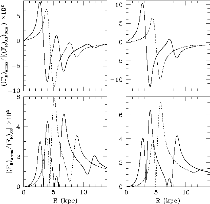
Figure 5: Radial force due to the spiral arms scaled by the absolute value of the A&S force at the Solar position (upper frames), and relative force perturbation (lower frames) in a model with $M_{S}/M_{D}$ = 0.0175. Left-hand frames: model with the spiral locus of Fig. 1; right-hand frames: model with the spiral locus pf Fig. 2. Values are given along the positive $x^{\prime}$ (continuous lines) and $y^{\prime}$ (dotted lines) axes defined in Fig. 10.

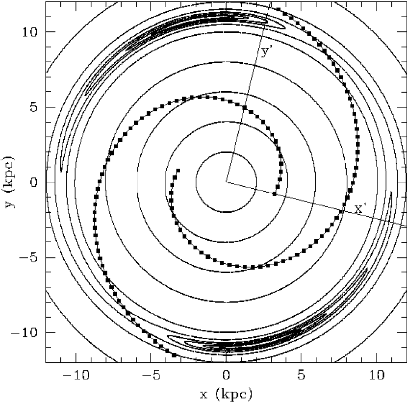
Figure 10: Some equipotential curves ${\Phi}_{eff}$ = const. for a model with $M_{S}/M_{D}=0.0175$, ${\Omega}_{p}$ = 20 km s^-1 kpc^-1, and the spiral locus in Figure 2. The inertial $x,y$ and non-inertial $x^{\prime},y^{\prime}$ axes are shown. Each square marks the center of an oblate spheroid.

Figure 5 plots the radial force produced by the spiral arms in our model and the corresponding relative force perturbation, as functions of galactocentric distance R. In this figure the mass ratio is $M_{S}/M_{D}$ = 0.0175 and $p_{0}$(R) has the exponential fall with a scalelength of 2.5 kpc; similar results are found with the linear fall of $p_{0}$(R). In the left frames of the figure the model has the spiral locus in Figure 1; in the right frames the spiral locus is that of Figure 2. In each case, the radial force (scaled by the absolute value of the force given by the A&S model at the Solar position) and the relative force perturbation are given along two radial lines (we call these two lines the $x^{\prime}$ and $y^{\prime}$ axes, respectively; see Figure 10): the line passing through the starting points of the spiral arms (continuous curves in the figure), and the line at right angles (dotted curves in the figure). The radial force, in the upper frames, shows the sign changes along the two chosen radial directions. The relative force perturbation is shown in the lower frames. Similar figures are obtained in the cases $M_{S}/M_{D}$ = 0.03 and 0.05, showing the corresponding peak values quoted above for the relative force perturbation.

We made a preliminary study of self-consistency in the models of Figure 5, using the two values of ${\Omega}_{p}$, 15 km s^-1 kpc^-1 and 20 km s^-1 kpc^-1. We followed the method of C&G86 to obtain the density response to the given spiral perturbation. This method assumes that the stars with orbits trapped around an unperturbed circular orbit, and with the sense of rotation of the spiral perturbation, are also trapped around the corresponding central periodic orbit in the presence of the perturbation. Thus, we computed a series of central periodic orbits, and found the density response along their extension, using the conservation of mass flux between any two successive orbits. The initial circular orbits were taken with a separation of 0.25 kpc. For more details see C&G86.

We found the position of the maxima density response along each periodic orbit, and thus the positions of the response maxima on the Galactic plane are known. These positions are to be compared with the center of the assumed spiral arms, i.e. the spiral locus.

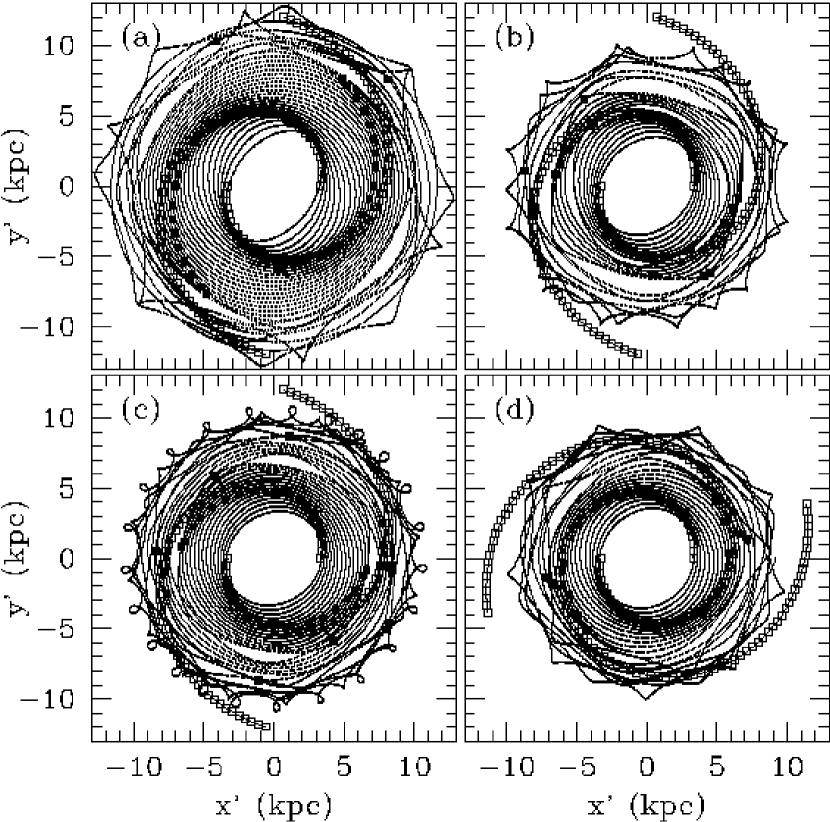
Figure 6: Response maxima (black squares) in models with the spiral loci (open squares) in Fig. 2 (frames (a),(b),(c)), and in Fig. 1 (frame (d)). ${\Omega}_{p}$ = 15 km s^-1 kpc^-1 in case (a); ${\Omega}_{p}$ = 20 km s^-1 kpc^-1 in cases (b),(c),(d). $M_{S}/M_{D}$ = 0.0175 in cases (a),(b),(d); $M_{S}/M_{D}$ = 0.00875 in case (c). Periodic orbits calculated following the C&G86 method are also shown.

Figure 6 illustrates some results. This figure shows the positions of the response maxima (black squares), along with the spiral arms (open squares), and the periodic orbits used in the method. Cases (a), (b), (c) have the spiral locus of Figure 2, and case (d) the spiral locus of Figure 1. The value of ${\Omega}_{p}$ is 15 km s^-1 kpc^-1 in case (a), and 20 km s^-1 kpc^-1 in cases (b), (c), (d). The mass ratio is $M_{S}/M_{D}$ = 0.0175 in cases (a), (b), (d), and $M_{S}/M_{D}$ = 0.00875 in case (c).

Figure 6 shows that mostly the response maxima lag behind the spiral arms, as the galactocentric distance increases. This behavior has already been discussed by C&G88 and PC&G: the response maxima may lag behind or ahead the spiral arms, depending on its radial scalelength and strength, among other parameters. PC&G give a nonlinear self-consistent model for the spiral galaxy NGC 1087, in which the response maxima lag behind, and claim that this is consistent with observations. C&G88 show that if they consider a dispersion of velocities around the central periodic orbits, the displacement between the response maxima and the spiral arms diminishes, obtaining a better self-consistency.

Once we found the positions of the response maxima, with the density response along each central periodic orbit we computed the average density response ${\rho}_{resp}$ around each one of these positions, taking a circular vicinity of radius equal to the semi-axis $a_{0}$ of the spheroids in the model. We then compared ${\rho}_{resp}$ with the imposed density, i.e. the one proposed by the model. This imposed density, ${\rho}_{mod}$, is the sum of the A&S disk density on the Galactic plane and the central density of the spiral arms. ${\rho}_{mod}$ is computed $along$ the arms. The densities ${\rho}_{resp}$ and ${\rho}_{mod}$ are compared at a same galactocentric distance $R$, but the corresponding positions on the Galactic plane may differ in azimuth, as shown in Fig. 6.

Following C&G88 and A&L, we computed the ratio ${\rho}_{resp}$/${\rho}_{mod}$ to analyze the self-consistency of the assumed spiral perturbation. This ratio should be close to 1. Figure 7 shows the value of this ratio for each case in Fig. 6. Figure 7(a), with ${\Omega}_{p}$ = 15 km s^-1 kpc^-1, shows a high density response in the inner region where the spiral arms begin. This behavior has been discussed by C&G86 and C&G88. However, Figures 7(b),(c),(d), with ${\Omega}_{p}$ = 20 km s^-1 kpc^-1, show a lower response in the inner region, making the ratio ${\rho}_{resp}$/${\rho}_{mod}$ be closer to 1. Thus, in this preliminary analysis, we favor ${\Omega}_{p}$ = 20 km s^-1 kpc^-1. In contrast, A&L found (for their model) that the density response could not favor a specific value of ${\Omega}_{p}$.

Case (c) in Fig. 7 shows a better self-consistency than case (b), which has twice the mass in the spiral arms. In both cases the density response differs strongly from the imposed density in the region around the distance (7 kpc) of the corresponding 4/1 resonance. Case (d), with the spiral locus of Fig. 1, appears to give an acceptable density response, even in the region of the 4/1 resonance.

The approximately self-consistent four models (a)-(d) of Figs. 6 and 7 have mass in the spiral arms seemingly in the lower limit of the interval (from Fig. 15 of PC&G) which an Sb galaxy like ours needs to sustain a nonlinear, self-consistent spiral perturbation. The analysis for self-consistency is also needed around the upper limit of the mass ratio $M_{S}/M_{D}$. As the method of C&G86 gives only approximate results (C&G88), this analysis and the preliminary results given above need to be reconsidered using the suggested improvements for self-consistency found by C&G88: it may be necessary to account for a population of orbits around the periodic orbits, with an appropriate velocity dispersion, and perhaps also the inclusion of four-armed spirals (A&L, Lépine, Mishurov, & Dedikov 2001). In a study currently underway, we are exploring the self-consistency of our models considering these components, with the mass ratio $M_{S}/M_{D}$ in the suggested interval, with other density laws in the oblate spheroids, and taking the dimensions $a_{0}$, $c_{0}$ as functions of galactocentric distance. A 3D orbital analysis as the one made by Patsis & Grosbøl (1996) would be also relevant in this procedure.

4 A COMPARISON WITH THE TIGHT-WINDING APPROXIMATION

In the tight-winding approximation for the spiral arms (e.g., Binney & Tremaine 1994), the potential at a given point is determined by the properties of the spiral arms in a small vicinity around the point. This approximation is given by Eq. (1) in the case of a two-armed spiral pattern. In our model, the potential at any point in space is obtained by summing the contributions of every element of mass along the spiral arms. Thus, a comparison of our model with the tight-winding model has some interest.

In Figure 8 we give the potential and radial force, scaled by the absolute value of the potential and radial force of the A&S model at the Solar position, of a model (continuous line) with the spiral locus in Figure 2, a mass ratio $M_{S}/M_{D}$ = 0.0175, and an exponential fall of the central density in spheroids, $p_{0}$(R), with a radial scalelength of 2.5 kpc. We plot the potential and radial force of the spiral arms along three radial lines: the positive $x^{\prime}$ axis (upper frames), and the lines at 60^∘ (middle frames) and 120^∘ (lower frames) from the $x^{\prime}$ axis (in the direction toward the $y^{\prime}$ axis). The dotted line shows the corresponding potential and radial force of a tight-winding model, i.e., Eq. (1), with the same spiral locus as in our model (Fig. 1), and with an amplitude f(R) (Eq. (1)) of the form considered by C&G86: f(R) = -AR$e^{-{\epsilon}_{s}R}$. In Figure 8 we take A = 450 km² s^-2 kpc^-1 and ${\epsilon}_{s}$ = 1/2.5 kpc^-1 (that is, the same radial scalelength as in our model). The high 15.5^∘ pitch angle of the spiral locus is not suitable for a rigorous comparison, but we see that our model cannot be well-approximated by a tight-winding model. Notice, for instance, in the upper right frame of Figure 8 the effect of the mass in the spiral arms inner to $\sim$ 8 kpc: the attraction of the whole spiral pattern requires that the point at which the radial force changes from negative to positive needs to be closer to the spiral arm around 8 kpc than in the tight-winding model. This accumulated negative radial force shifts the net force toward negative values in the outer regions.

In Figure 9 we compare the radial forces along the positive $x^{\prime}$ axis, for models with a 3^∘ pitch-angle, two-armed, spiral locus starting at 3.3 kpc. The continuous line gives our model with $a_{0}$ = 0.1 kpc, $c_{0}$ = 0.05 kpc, separation of spheroids’ centers of 0.05 kpc, a low mass ratio $M_{S}/M_{D}$ = 0.001, and an exponential fall of $p_{0}$(R) with a radial scalelength of 2.5 kpc. The dashed line results from a tight-winding model with A = 9 km² s^-2 kpc^-1 and ${\epsilon}_{s}$ = 1/2.5 kpc^-1. Both models are similar in the inner region, but as the galactocentric distance increases the effect mentioned above begins to be important. Even in this low-mass case, the attraction of all the mass in the spiral arms makes the radial force in the outer regions asymmetric around zero; in fact, at large distances this force (per unit mass) is -$GM_{S}/R^{2}$. In Section 6 we discuss briefly some consequences of these results, which must have important consequences to the gas dynamics.

5 ORBITAL ANALYSIS

As an application of our model, we have made a brief study of stellar orbits in the Galactic plane. Poincaré diagrams are presented, and discussed from the perspective of the sense of orbital motion defined in the Galactic inertial frame and its connection to the onset of stochastic motion. To investigate further the nature of chaotic motion apparent in Poincaré diagrams, we utilized additionally Lyapunov exponents (Wolf 1984).

5.1 Poincaré Diagrams and the Separatrix of Zero Angular Momentum

The orbital analysis is made in the non-inertial reference frame attached to the spiral pattern, labeled as the primed system of Cartesian coordinates $(x^{\prime},y^{\prime},z^{\prime})$. As defined in Section 3, the $x^{\prime}$ axis is taken as the line passing through the inner starting points of the spiral arms; the $z^{\prime}$ axis is perpendicular to the Galactic plane, with its positive sense toward the north Galactic pole, and the $y^{\prime}$ axis is such that the $(x^{\prime},y^{\prime},z^{\prime})$ axes form a right-hand system. The angular velocity of the spiral arms, ${\Omega}_{p}$, points in the negative direction of the $z^{\prime}$ axis, i.e., a clockwise rotation.

In the Galactic plane the effective potential in the non-inertial frame is given by

$${\Phi}_{eff}(x^{\prime},y^{\prime})={\Phi}_{AS}(x^{\prime},y^{\prime})+{\Phi}_{s}(x^{\prime},y^{\prime})-(1/2){\Omega}_{p}^{2}(x^{\prime 2}+y^{\prime 2}),$$ (5)

with ${\Phi}_{AS}$ the A&S potential and ${\Phi}_{s}$ the potential due to the spiral arms.

Figure 10 shows some equipotential curves ${\Phi}_{eff}$ = const. for the model with $M_{S}/M_{D}=0.0175$, ${\Omega}_{p}$ = 20 km s^-1 kpc^-1, exponential fall of $p_{0}$(R), and the spiral locus in Figure 2 (i.e., $i_{p}$=15.5^∘). Both figures 2 and 10 have the same orientation of the spiral pattern. The inertial $x,y$ and non-inertial $x^{\prime},y^{\prime}$ axes are shown in Figure 10. Each square traces the center of an oblate spheroid, and the islands in the equipotential curves appear at the corotation distance (10.9 kpc in this case).

A known integral of stellar motion in the non-inertial system is Jacobi’s expression $E_{J}$ = $(1/2){\rm{\boldmath v^{\prime}}}^{2}+{\Phi}_{eff}$, with ${\bf v}^{\prime}$ the velocity in this system. Then the equipotential curves are curves of zero velocity for corresponding values of $E_{J}$. Figure 11 plots the value $E_{J}$ = ${\Phi}_{eff}$ on the positive $x^{\prime}$ axis, for the model in Figure 10.

Poincaré diagrams were constructed following the usual procedure. We found the crossing points with the $x^{\prime}$ axis of orbits with a given value of $E_{J}$, and made Poincaré diagrams $x^{\prime}$ vs $v_{x}^{\prime}$ for the crossing points having $v_{y}^{\prime}>0$ . All the crossing points with $v_{y}^{\prime}<0$ were incorporated in the $v_{y}^{\prime}>0$ diagrams taking $x^{\prime}\rightarrow-x^{\prime}$ , $v_{x}^{\prime}\rightarrow-v_{x}^{\prime}$. We studied several models with a two-armed spiral pattern, taking combinations of ${\Omega}_{p}$ (15 or 20 km s^-1 kpc^-1), $i_{p}$ (11^∘ or 15.5^∘), $M_{S}/M_{D}$ (0.0175, 0.03, or 0.05), and the function $p_{0}$ (linear or exponential). Also, we studied models with the $six$ spiral arms in Figure 3, taking combinations of ${\Omega}_{p}$ = 20, 60 km s^-1 kpc^-1, $M_{S}/M_{D}$ = 0.0175, 0.05, and an exponential function $p_{0}$. In all cases the orbits were computed with a Bulirsch-Stoer algorithm (Press et al. 1992), with a mean maximum error $|(E_{J_{final}}-E_{J_{initial}})/E_{J_{initial}}|$ of order $10^{-12}$, in runs with elapsed physical times of $10^{9}$ to $10^{11}$ years.

In this subsection we present Poincaré diagrams for models with the lower mass ratio $M_{S}/M_{D}$ = 0.0175; results with $M_{S}/M_{D}$ = 0.05 are presented in the next section.

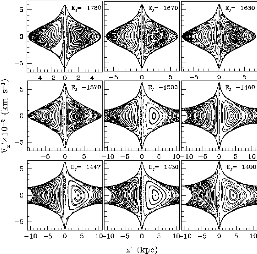
Figure 12: Poincaré diagrams for nine values of $E_{J}$ (in units of $10^{2}$ ${\rm km}^{2}~{}{\rm s}^{-2}$), in a model with the spiral locus of Fig. 2, $M_{S}/M_{D}=0.0175$, and ${\Omega}_{p}$ = 20 km s^-1 kpc^-1. In each plot the separatrix is shown with darker spots.

Figure 12 shows Poincaré diagrams for the model of Figures 10 and 11, i.e., ${\Omega}_{p}$ = 20 km s^-1 kpc^-1 and the spiral locus in Figure 2 ($i_{p}$=15.5^∘). Values of $E_{J}$ were selected in the interval [-1.8, -1.2]$\times$ $10^{5}$ km² s^-2. In this and following figures each diagram was constructed with approximately fifty orbits. The boundary of the permitted region begins to open at the value $E_{J}$ of the island around the corotation distance (see Figure 10) to which the $x^{\prime}$ axis is tangent. This value of $E_{J}$ is the maximum of the curve in Figure 11.

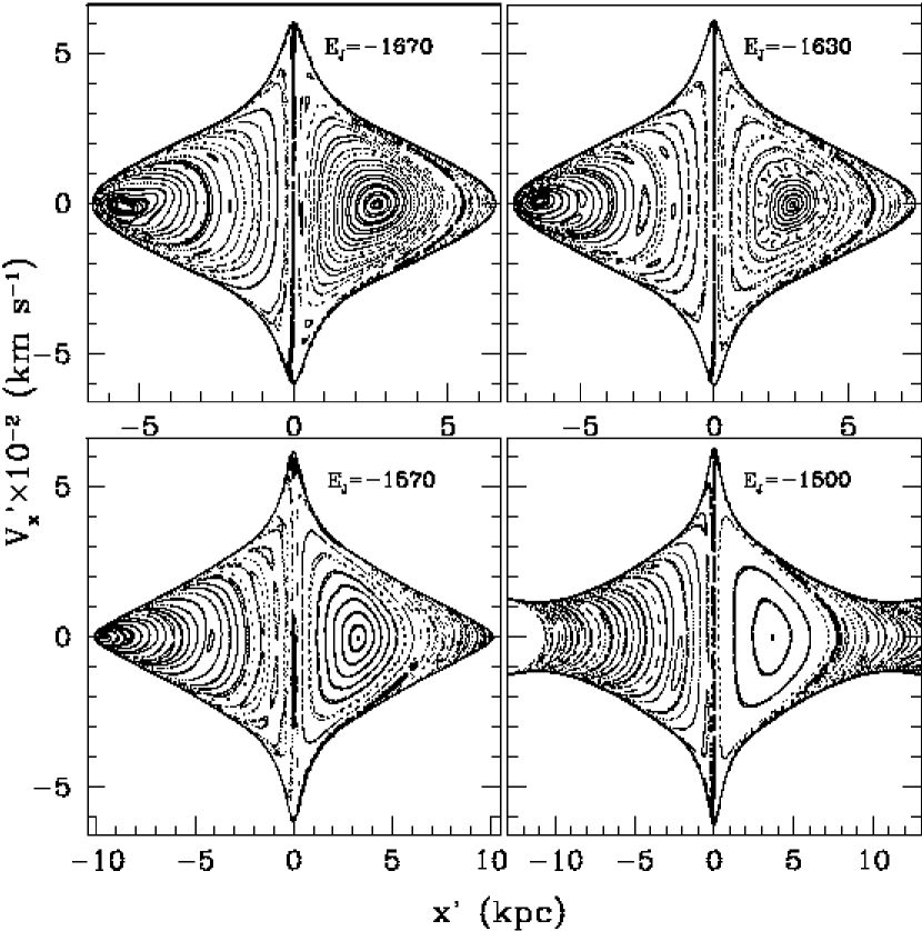
Figure 13: Poincaré diagrams in a model with the six spiral arms in Fig. 3, and $\Omega_{p}=20$ km s^-1 kpc^-1. The two K-band arms and the four optical arms have the same mass ratio $M_{S}/M_{D}=0.0175$. The separatrix is shown with darker spots.

Figure 13 gives four Poincaré diagrams for a model with the six spiral arms in Figure 3, and again ${\Omega}_{p}$ = 20 km s^-1 kpc^-1. In this example the mass ratio for the two, K-band, spiral arms is $M_{S}/M_{D}$ = 0.0175, and the total mass in the four optical arms has this same ratio; i.e. the total mass in the four optical arms is equal to the total mass in the two K-band arms.

In the two Poincaré diagrams shown in Figures 14 and 15, we keep the same spiral pattern arms as in Figure 13, but take the high pattern speed ${\Omega}_{p}$ = 60 km s^-1 kpc^-1. Figure 16 shows some ${\Phi}_{eff}$ = const. curves for this case. The black squares give the four optical arms, and the open squares the two K-band arms. The $x^{\prime}$ axis in this case of six arms is the starting line of the two K-band arms. The islands in the ${\Phi}_{eff}$ = const. curves appear at a lower corotation distance (c.f., Figure 10). Figure 17 gives $E_{J}$ = ${\Phi}_{eff}$ on the positive $x^{\prime}$ axis.

The orbital structure of Poincaré diagrams shown in Figures 12 to 15, is the usual structure obtained in studies of stellar orbits in spiral and barred galaxies (e.g., Contopoulos 1983, Athanassoula et al. 1983, Teuben & Sanders 1985). A dominant periodic orbit appears in the $x^{\prime}>0$ side of each diagram, and in some cases (i.e., for a certain range in $E_{J}$) there is also a dominant periodic orbit on the $x^{\prime}<0$ side. Rather than a detailed analysis of the orbital structure, what we wish to emphasize in these diagrams is the clear separation of two regions, each one containing orbits with a definite sense of rotation, prograde or retrograde, defined in the Galactic inertial frame. In our situation the spiral pattern moves in the clockwise sense; so the usual definition in the non-inertial frame (e.g., Athanassoula et al. 1983) would call prograde orbits those orbits crossing the $x^{\prime}<0$ side, and retrograde orbits those crossing the $x^{\prime}>0$ side. This definition is ambiguous, because the azimuthal velocity in the non-inertial frame may change sign along a given orbit. Thus, an orbit may be both prograde and retrograde (Contopoulos 1983). On the other hand, in the inertial frame, and for the considered range of strengths of the spiral perturbation, orbits maintain the sign of their azimuthal velocities, with the exception of orbits with angular momentum close to zero (as computed in this frame).

We define the sense of orbital rotation in the inertial frame, as follows: prograde if the azimuthal velocity is always of the same sign as the angular velocity of the spiral pattern, $\Omega_{p}$; and retrograde if the azimuthal velocity always has the opposite sign of $\Omega_{p}$. With this definition, Poincaré diagrams show a sharp separation between the regions of prograde and retrograde orbits by a “curve” that we call the separatrix of zero angular momentum, which corresponds to orbits with nearly vanishing angular momentum in the inertial frame. In Figures 12 to 15, the separatrix is shown with darker spots. The orbits forming this “curve” would need to be computed over a longer time to fill it in the diagrams where it appears to be discontinuous.

The definition of sense of orbital motion in the inertial frame reveals that all orbits inside the region bounded by the separatrix are retrograde. Prograde orbits are outside this region. Prograde orbits may have points on both the $x^{\prime}>0$ and $x^{\prime}<0$ sides of a Poincaré diagram. Another way of saying this is that only prograde orbits may change their sense of motion in the rotating frame. The separatrix is the transition region between prograde and retrograde orbits in the inertial reference frame.

In Figure 15 the prograde region has orbits with appreciable chaotic motion. This behavior is discussed in more detail in the next subsection.

We have stressed above that the definition of sense of orbital rotation in the Galactic inertial frame is useful, as long as the strength of the spiral perturbation is not too high. From our study, the correlation chaos-prograde motion seems valid to our Galaxy. In the next section we analyze the orbital structure in the case of the higher mass ratio $M_{S}/M_{D}$ = 0.05 still applicable to our Galaxy in our framework. We will see that the separatrix increases its width, i.e., the number of orbits which are both prograde and retrograde in the inertial frame increases. However, our definition still provides a clear separation of prograde and retrograde orbits. An interesting situation in which this definition apparently loses its usefulness is the case of lopsided galaxies considered by Noordermeer, Sparke, & Levine (2001). In this case it is expected that even in the inertial frame there is a wide region of orbits that are both prograde and retrograde.

Defining the sense of orbital motion in the inertial frame has a more physical connection with the character of orbits affected by a spiral perturbation. As we will see in the next section, the analysis of Poincaré diagrams based on this definition shows a connection with the onset of chaotic motion.

5.2 Exploring the Nature of Orbital Chaos

Orbital chaos has been found in potentials including spiral or bar perturbations (e.g., Contopoulos 1983, Athanassoula et al. 1983, Pfenniger 1984, Teuben & Sanders 1985, Fux 2001), and in other non-axisymmetric potentials (e.g., Alvarellos 1996; Noordermeer, Sparke, & Levine 2001). In this subsection we present some results related with the onset of chaotic stellar motion in our model, taking the higher mass ratio $M_{S}/M_{D}$ = 0.05, which we consider applicable in our Galaxy. We find that as the mass ratio $M_{S}/M_{D}$ increases, the onset of orbital chaos always occurs outside the region bounded by the separatrix defined in the previous section, i.e., the prograde region. Furthermore, within the plausible range of $M_{S}/M_{D}$, chaos is entirely confined to the prograde region.

In Figure 18 we give a Poincaré diagram with $E_{J}=-1630\times 10^{2}~{}{\rm km}^{2}{\rm s}^{-2}$, (previously shown in Figure 12, with $M_{S}/M_{D}$ = 0.0175), and in Figure 19 a diagram with the same value of $E_{J}$, but now with $M_{S}/M_{D}$ = 0.05. In both cases the pattern speed is ${\Omega}_{p}$ = 20 km s^-1 kpc^-1. A comparison of the two figures shows that increasing the strength of the spiral perturbation causes the separatrix to increase in width, and also some chaotic motion begins to appear on the $x^{\prime}<0$ side in Figure 19, i.e., outside the region bounded by the separatrix.

To investigate the orbital chaos which appears in Figure 19, we did a Lyapunov exponents analysis following Wolf (1984), by calculating individual orbits in the diagram in Figure 19. The first Lyapunov exponent was calculated to classify orbits as chaotic or non-chaotic by applying the usual criterion for chaos, namely $\lambda>0$ for chaotic motion (which means that two orbits with very close initial conditions, will increase their relative distance as $e^{\lambda t}$, with $t$ the time), and $\lambda\leq 0$ for regular motion (where the relative distance will be constant or decrease exponentially to zero). We found that the exponent $\lambda$ in the prograde region, in the scattered-points subregions, such as that marked with the number 1 in Figure 19, is always positive ($\gtrsim.4$) for each pair of orbits we tried, as expected for conservative chaos. On the other hand, this exponent is less than zero for orbits in the regular regions of the Poincaré diagram for both prograde and retrograde orbits (marked with numbers 2 and 3, respectively). Thus, chaotic motion is entirely confined to the prograde orbits (seen from the inertial frame) for plausible parameters for the spiral arms in the Galaxy.

If we further increase the mass ratio $M_{S}/M_{D}$, we find that chaotic motion is important for a range of values of $E_{J}$, and it spreads from the prograde region toward the retrograde region; This behavior was seen in previous orbital studies (e.g. Contopoulos 1983, Athanassoula et al. 1983, Teuben & Sanders 1985), although not linked with the sense of orbital motion defined in the inertial frame.

Figure 20 shows the effect which produces the addition of the four optical arms to the two K-band arms considered in Figure 19, the total mass in the optical arms being the same as the mass in the K-band arms. There are structural similarities between both diagrams (Figs. 19 and Fig. 20), but the main difference is the wider separatrix in Figure 20. In the separatrix the Lyapunov exponent is negative; thus, chaos is still confined to the prograde region.

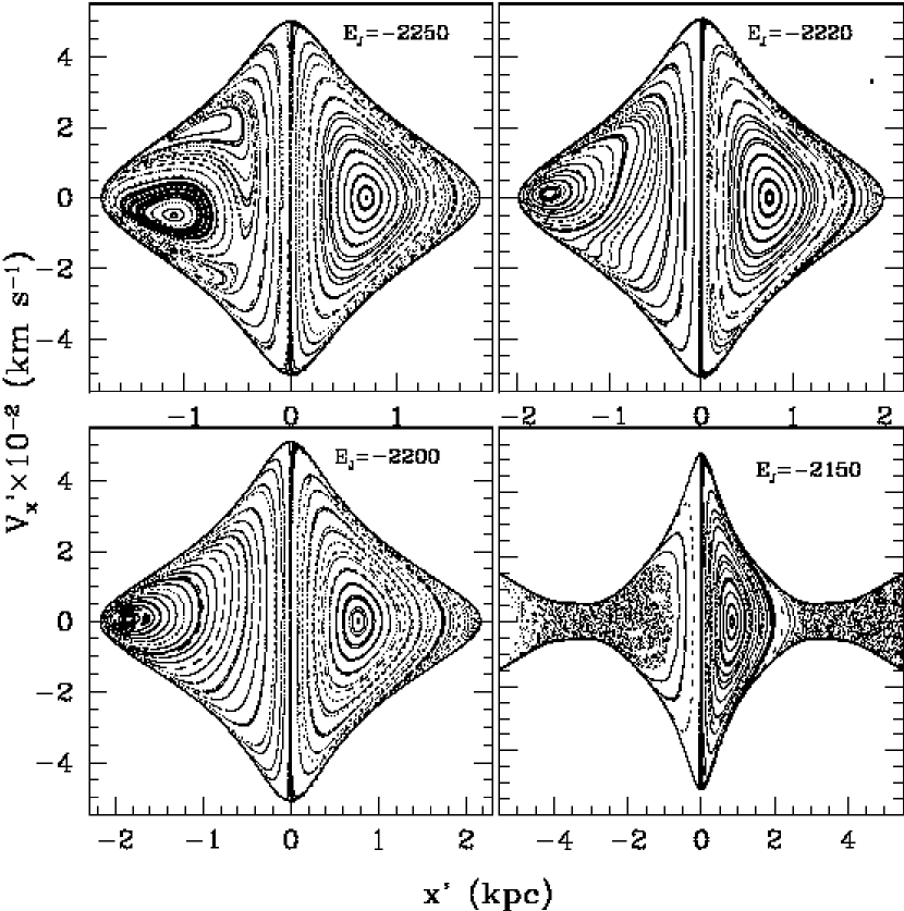
Figure 21: Some Poincaré diagrams in a model with the six spiral arms in Fig. 3. $\Omega_{p}=60$ km s^-1 kpc^-1, and $M_{S}/M_{D}=0.05$ for both optical and K-band arms. The separatrix is shown with darker spots.

In Figure 21 we give four Poincaré diagrams for the model with six spiral arms in Figure 20, but now with ${\Omega}_{p}$ = 60 km s^-1 kpc^-1. The prograde and retrograde regions are separated by a narrow separatrix. The first three diagrams show non-chaotic motion within corotation distance (see Figures 4 and 16). The fourth diagram, in the lower right frame, shows pervasive chaos in a wide zone in the prograde region. This corresponds to stellar motion that can surpass the corotation barrier. The same behavior is obtained in the case shown in Figure 15, with a lower mass in the six spiral arms. This transition from regular to chaotic motion was also obtained by Fux (2001), who considered the Galactic bar as the perturbating agent.

All these results show that the onset of chaotic motion starts in the prograde region. The prime cause for chaotic motion is the onset of bifurcations and resonance interactions (Contopoulos 1967, Martinet 1974, Athanassoula et al. 1983, Athanassoula 2001). Regarding the resonance interactions, Figure 22 shows some important resonance curves for nearly circular retrograde orbits in the A&S Galactic model; in particular, with the ${\Omega}_{p}$ = 20 km s^-1 kpc^-1 line given in the figure (corresponding to the pattern speed of a spiral perturbation rotating in the prograde sense), the corresponding resonance positions can be read on the R axis. Thus, resonances for retrograde orbits are more widely separated, as compared with the resonances for prograde orbits, some of which are shown in Figure 4; i.e., resonance interactions are more important in prograde orbits.

6 DISCUSSION AND CONCLUSIONS

We present a 3D model for a spiral mass distribution, consisting of inhomogeneous oblate spheroids superposed along a given spiral locus. The model is applied in particular to our Galaxy, but can easily be applied to spiral galaxies in general. Furthermore, it allows to look with a deeper physical insight into details that are inaccessible to the classical treatment of the spiral perturbation, which models it as a simple periodic function. Our model of oblate spheroids is physically simple and plausible, with continuous derivatives and density laws.

In our Galaxy, the model parameters, such as the number of spiral arms, its pitch angle, its radial extent, the pattern speed, the dimensions and mass density of the spheroids, and the total mass in the arms, were taken in a range of possibilities suggested by observations and theory.

In principle, the dimensions and mass density of the oblate spheroids will depend on the type of spiral arms which are modeled, gaseous or stellar. In this first work the adopted dimensions resemble those of gaseous spiral arms (Kennicutt & Hodge 1982), and a linear density law in the spheroids has been considered. We assembled Galactic models with two-armed spirals, such as the 15.5^∘ pitch-angle, stellar arms discussed by Drimmel (2000), and with $six$ spiral arms: adding the four 12^∘ pitch-angle, optical arms, delineated by luminous HII regions. From a range of possibilities, we considered three values of the pattern speed: ${\Omega}_{p}$ = 15, 20, and 60 km s^-1 kpc^-1, and the ratio of the mass in the spiral arms to the disk’s mass in the A&S axisymmetric Galactic model, $M_{S}/M_{D}$, in the range 0.0175 to 0.05 . In this range of masses the average force due to the spiral arms is between 5 and 10 $\%$ of the background axisymmetric force.

In an effort to achieve a self-consistent model of the spiral perturbation in our Galaxy, we have used the well-known, approximate method of C&G86 to analyze the density response to this imposed perturbation. We have computed the density response in a Galactic potential with two spiral arms, taking the pattern speed as ${\Omega}_{p}$ = 15 and 20 km s^-1 kpc^-1, and the mass ratio $M_{S}/M_{D}$ around the lower limit given above. Our nearly self-consistent models favor the pattern speed of 20 km s^-1 kpc^-1. However, this preliminary analysis must be improved at least accounting for (a) a hot stellar population around the central periodic orbits, (b) a four-armed, stellar, spiral pattern in the density response, in addition to the main two-armed component (A&L), and (c) a properly modeling of the dimensions of two-armed stellar spirals, as the K-band arms given by Drimmel (2000); this type of arms is azimuthally broad (Rix & Zaritsky 1995), thus an increase with galactocentric distance of the major semi-axis $a_{0}$ of spheroids would be appropriate. This analysis will be presented in a future work.

Modeling of the gravitational potential produced by a spiral perturbation has usually been based on the tight-winding approximation (TWA, Eq. 1). We have compared the potential and force fields of a two-armed spiral perturbation given by our model with a TWA model. We found that the self-gravity of the spiral pattern (i.e. contributions to the potential from the entire pattern), which is not accounted for in the TWA (which acts more like a local approximation), cause the local spiral potential to adopt shapes that are not correctly fit by the simple perturbing term that has been traditionally invoked to represent the local spiral potential. This fact may have far-reaching consequences; for instance, in the gas response to the spiral perturbation. We have performed modest 1D MHD simulations (Franco, Martos & Pichardo 2001) with the code Zeus to show the differences in the gas response using the conventional model of a cosine for the potential and the model presented in this work. These simulations show that shocks do not leave the arm downstream as in previous calculations (Baker & Barker 1974, Martos & Cox 1998) for a plausible range of entry speeds. And, in correspondence with observational expectations, shocks seek the upstream edge of the arm, i.e. the concave side inside corotation marked in optical observations of galaxies for accumulations of dust in the inner part of the spiral arms. The inclusion of the magnetic field is essential to this effect. In this manner, results based on the TWA should be revised: the gas response depends strongly on the position in the Galaxy. A potential “well” in the arm may disappear as such at a different segment of the arm.

In the analysis of Poincaré diagrams we found it is quite fruitful to use an inertial frame to define the prograde or retrograde sense of orbital motion around the Galactic center along with the usual definition in the non-inertial system, where the Poincaré diagrams are defined. In the inertial frame the sense of motion is preserved with time for almost every orbit in our experiments exception being orbits with nearly zero angular momentum. This property relies upon the parameters we consider plausible for our Galaxy. If we include information of the inertial system in the non-inertial one, Poincaré diagrams reveal that prograde and retrograde orbits, as defined in the inertial frame, occupy sharply separated regions, through a separatrix corresponding, loosely, to nearly zero angular momentum orbits in this system.

The definition of sense of orbital motion in the inertial frame goes beyond a mere matter of semantics, for it has a simple physical meaning and it appears to be intimately connected to the onset of chaos. Based on an analysis of Poincaré diagrams and the first Lyapunov exponent we find that, within plausible amplitudes and pitch angles of the spiral arms for a Galaxy such as the Milky Way (and independently of the number of arms chosen), if there is chaos, only prograde orbits can exhibit it, and for a sufficiently weak perturbation, as it seems to be the case in our Galaxy, the separatrix is a well-defined narrow curve. The onset and extension of chaotic subregions of the prograde region, depends on two main parameters that are the mass in the spiral arms or the relative force; and the angular velocity. We stress out the point that the standard definition in the rotating frame, which calls the $x^{\prime}>0$ of the diagram the retrograde side, and $x^{\prime}<0$ the prograde side (for a spiral pattern moving clockwise), would not have shed light onto the connection chaos-prograde motion, since the same orbit (ordered or chaotic) can occupy both sections of Poincaré diagrams. The different behavior regarding the onset of chaos of prograde and retrograde orbits, as defined in the inertial system, could be attributed to the overlapping of resonances (Contopoulos 1967, Athanassoula 2001). Figures 4 and 22 show that the spacing of the main resonances is wider for retrograde orbits, and is even smaller if we take higher angular velocities for the spiral pattern. In cases with the lower spiral masses ($M_{S}/M_{D}\lesssim.03$), we do not find chaos for angular speeds of the spiral pattern lower than 20 km s^-1 kpc^-1. We have also computed some orbital families with $\Omega_{p}=60$ km s^-1 kpc^-1 since n-body models predict thoses velocities (that corresponds to the bar), and we find that, even for the lowest spiral mass we considered, chaos appears for some families (Fig. 21, $E_{J}=-2150\times 10^{2}$ km² s^-2), where almost all the prograde region is chaotic but chaos do not invade retrograde region. The inclusion of more than two spiral arms does not seem change dramatically the results (Figs. 19 for two arms and 20 for 6 arms). A minimum strength of the perturbation is required for the appearance of stochastic motion in the models with the lowest angular speeds (15 and 20 km s^-1 kpc^-1). We find that the amplitude of approximately 6$\%$ (in average) of the axisymmetric radial force is required (that corresponds in our model to a $M_{S}/M_{D}\lesssim.05$ for a pitch angle of 15.5^∘). For cases of very strong spiral perturbations (relative forces higher than 15$\%$) the separatrix is no longer a well-defined curve and chaos is pervasive. However we don’t think this spiral forcing is proper for a Sb galaxy.

It is worth noticing that our results are valid in the plausible range of parameters (and even in unrealistic cases with maximum relative forces for the spiral arms up to 15$\%$) in a galaxies similar to the Milky Way, with 2, 4 or 6 arms. However, our results will surely be altered by the influence of the Galactic bar. We are currently studying this effect.

Figure 1: Spiral arms in our Galaxy (Fig. 2 of Drimmel 2000). Optical arms (black squares) and K-band arms (open squares). Continuous line: first of three spiral loci considered to model the spiral arms.

Figure 2: Only the K-band spiral arms. The continuous line is our second spiral locus. We consider the region $R\geq 3.3$ kpc, traced by the black squares.

Figure 3: Spiral arms in our Galaxy. Optical arms (black squares) and K-band arms (open squares). Continuous line: is our fit to a four-armed locus. The third locus we considered is composed by the two locus joined, our fit to K-band arms (shown in the previous figure) and the four-armed locus presented in this Figure.

Figure 4: Some resonance curves in the A&S Galactic model. The lines ${\Omega}_{p}$ = 15 and 20 km s^-1 kpc^-1 are shown in the figure.

Figure 7: The ratio of the response density to the imposed density along the arm, ${\rho}_{resp}/{\rho}_{mod}$, as a function of galactocentric distance, for each case in Fig. 6.

Figure 8: Potential and radial force, scaled by the absolute value of the potential and force of the A&S model at the Solar position, of a model (continuous line) with the spiral locus in Fig. 2, a mass ratio $M_{S}/M_{D}$ = 0.0175, and an exponential fall (in the central density of the spheroids along the spiral arm) with scalelength of 2.5 kpc. The potential and radial force of the spiral arms along three radial lines are given, one along the positive $x^{\prime}$ axis (upper frames), and the other two along the lines at 60^∘ (middle frames) and 120^∘ (lower frames) from the $x^{\prime}$ axis (in the direction toward the $y^{\prime}$ axis). The dotted lines show the corresponding potential and radial force of a tight-winding model, with the same spiral locus as in our model of Fig. 1.

Figure 9: Comparison of the radial forces due to a 3^∘ pitch-angle, two-armed, low-mass, spiral perturbation. Our model is given by the continuous line; the dashed line represents a tight-winding model.

Figure 11: The value of $E_{J}$ along the $x^{\prime}$ axis for our model in Fig. 10.

Figure 14: Poincaré diagram with $E_{J}=-2200\times 10^{2}$ km² s^-2 in the model of six spiral arms and same parameters as in Fig. 13 but here with $\Omega_{p}=60$ km s^-1 kpc^-1.

Figure 15: Poincaré diagram with $E_{J}=-2050\times 10^{2}$ km² s^-2 and same conditions as in Fig. 14.

Figure 16: Some equipotential curves ${\Phi}_{eff}$ = const. for the model corresponding to Figs. 14 and 15. Black squares: optical arms; open squares: K-band arms.

Figure 17: The value of $E_{J}$ along the $x^{\prime}$ axis in Fig. 16.

Figure 18: Zoom of the Poincaré diagram with $E_{J}=-1630\times 10^{2}$ km² s^-2 in Fig. 12. Compare with next figure.

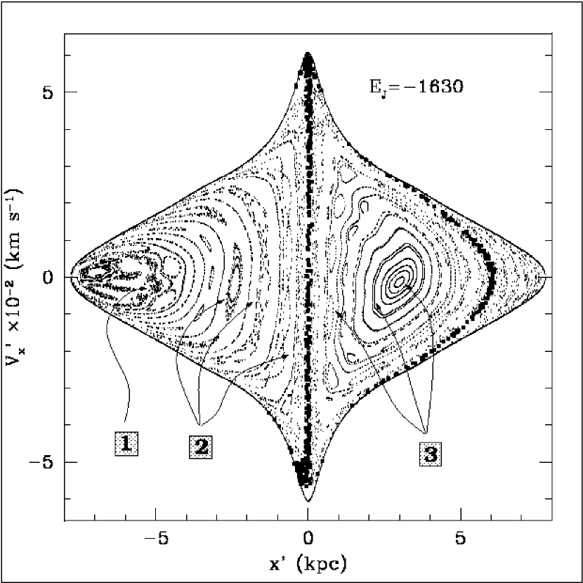
Figure 19: Poincaré diagram for the same value of $E_{J}$ and same parameters as in Fig. 18, but here with $M_{S}/M_{D}=0.05$. The arrows and numbers indicate some zones where we computed Lyapunov exponents.

Figure 20: Poincaré diagram with $E_{J}=-1630\times 10^{2}$ km² s^-2 in a model with the six spiral arms in Fig. 3. $\Omega_{p}=20$ km s^-1 kpc^-1, and $M_{S}/M_{D}=0.05$ for both optical and K-band arms. Compare with Fig. 19, which has the same ${\Omega}_{p}$ and $M_{S}/M_{D}$ in a model with the spiral locus in Fig. 2.

Figure 22: Some resonance curves for nearly circular retrograde orbits in the A&S Galactic model. The line $\Omega_{p}=20$ km s^-1 kpc^-1 is given in the figure. Compare with Fig. 4, which corresponds to nearly circular $prograde$ orbits.

References

- (1) Amaral, L.H., & Lépine, J.R.D., 1997, MNRAS, 286, 885 (A&L)
- (2) Athanassoula, E., Bienaymé, O., Martinet, & L., Pfenniger, D., 1983, A& A, 127, 349
- (3) Athanassoula, E., 2001, private communication
- (4) Alvarellos, J.L., 1996, Master Degree thesis, Univ. of California.
- (5) Allen, C., & Santillán, A., 1991, RMxAA, 22, 255 (A&S)
- (6) Baker, P.L. & Barker, P.K. 1974, A & A, 36, 179
- (7) Beck, R. 1993, IAUS, 157, 283
- (8) Binney, & J., Tremaine, S., 1994, Galactic Dynamics, 3rd edition (Princeton University Press)
- (9) Caswell, J.L., & Haynes, R.F. 1987, A & A, 171, 261
- (10) Contopoulos, G., 1967, Bull. Astr., Ser. 3, 2, 223
- (11) Contopoulos, G., 1983, A & A, 117, 89
- (12) Contopoulos, G. & Grosbøl, P., 1986, A & A, 155, 11 (C&G86)
- (13) Contopoulos, G. & Grosbøl, P., 1988, A & A, 197, 83 (C&G88)
- (14) Drimmel, R., 2000, A&A, 358, L13
- (15) Drimmel, R., & Spergel, D., 2001, ApJ, 556, 181
- (16) Englmaier, P. & Gerhard, O., 1999, MNRAS, 304, 512
- (17) Franco, J., Martos, M., Pichardo, B., 2002, ASP Conference Series, Eds. Athanassoula, E., Bosma, A., in press
- (18) Fux, R., 2001, A & A, 373, 511
- (19) Fux, R., 1998, A & A, 345, 787
- (20) Freudenreich, H.T., 1998, ApJ, 492, 495
- (21) Georgelin, Y.M., & Georgelin, Y.P., 1976, A&A, 49, 57
- (22) Gordon, M.A., 1978, ApJ., 222, 100
- (23) Grosbøl, P., 2001, private communication
- (24) Heiles, C. 1995, The Physics of the Interstellar Medium and Intergalactic Mediu m. ASP Conference Series, Vol. 80. Ed A. Ferrara, C.F. McKee, C. Heiles, P.R. Shapiro (Astronomical Society of the Pacific: San Francisco, California)
- (25) Heiles, C. 1996, ApJ, 462, 316
- (26) Kennicutt, R., Jr & Hodge, P., 1982, ApJ, 253, 101
- (27) Kikuchi, N., Korchagin, V., & Miyama, S. M., 1997, ApJ, 478, 446
- (28) Lépine, J.R.D., Mishurov, Yu.N., & Dedikov, S.Yu., 2001, ApJ, 546, 234
- (29) Lin, C.C., & Shu, F.H., 1964, ApJ, 140, 646
- (30) Lin, C.C., Yuan, C., & Shu, F.H., 1969, ApJ., 155,721
- (31) Martos, M.A., & Cox, D.P., 1998, ApJ, 509, 703
- (32) Martinet, L., 1974, A & A, 32, 329
- (33) Miyamoto, M., & Nagai, R., 1975, Pub.Astr.Soc.Japan, 27, 533
- (34) Noordermeer, E., Sparke, L., & Levine, S., 2001, MNRAS, 328, 1064
- (35) Palous, J., Ruprecht, J., Dluzhnevskaya, O.B., & Piskunov, T., 1977, A&A, 61, 27
- (36) Patsis, P.A. & Grosbøl, P., 1996, A & A, 315, 371
- (37) Patsis, P.A., Contopoulos, G., & Grosbøl, P., 1991, A & A, 243, 373 (PC&G)
- (38) Pfenniger, D., 1984, A&A, 134, 373
- (39) Press, W.H., Teukolsky, S.A., Vetterling, W.T. & Flannery, B.P., 1992, Numeric al Recipes in Fortran 77: The Art of Scientific Computing, 2nd. ed. (Cambridge University Press: Cambridge)
- (40) Rix, H. -W. & Zaritsky, D., 1995, ApJ, 447, 82
- (41) Roberts, W. W., Jr., Huntley, J. M., & van Albada, G. D., 1979, ApJ, 233, 67
- (42) Schmidt, M., 1956, B. A. N. 13, 15
- (43) Teuben, P.J. & Sanders, R.H., 1985, MNRAS, 212, 257
- (44) Vallée, J.P. 2002, ApJ, 566, 261
- (45) Vauterin, P., & Dejonghe, H., 1996, A&A, 313, 465
- Wolf (1984) Wolf, A., 1984, Quantifying Chaos with Lyapunov Exponents, Nonlinear Sci. Theory Appl. Ed. A.V. Holden, (Manchester Univ. Press.)