Wavefronts, Caustic Sheets, and Caustic Surfing in Gravitational Lensing

Abstract

Very little attention has been paid to the properties of optical wavefronts and caustic surfaces due to gravitational lensing. Yet the wavefront-based point of view is natural and provides insights into the nature of the caustic surfaces on a gravitationally lensed lightcone. We derive analytically the basic equations governing the wavefronts, lightcones, caustics on wavefronts, and caustic surfaces on lightcones in the context of weak-field, thin-screen gravitational lensing. These equations are all related to the potential of the lens. In the process, we also show that the standard single-plane gravitational lensing map extends to a new mapping, which we call a wavefront lensing map. Unlike the standard lensing map, the Jacobian matrix of a wavefront lensing map is not symmetric. Our formulas are then applied to caustic “surfing.” By surfing a caustic surface, a space-borne telescope can be fixed on a gravitationally lensed source to obtain an observation of the source at very high magnification over an extended time period, revealing structure about the source that could not otherwise be resolved. Using our analytical expressions for caustic sheets, we present a scheme for surfing a caustic sheet of a lensed source in rectilinear motion. Detailed illustrations are also presented of the possible types of wavefronts and caustic sheets due to nonsingular and singular elliptical potentials, and singular isothermal spheres, including an example of caustic surfing for a singular elliptical potential lens.

I Introduction

Among relativistic concepts of direct application to gravitational lensing, the observer’s past lightcone is perhaps the most fundamental. The lightcone concept unifies the temporal and spatial properties of lensing events in a geometrical manner that makes the multiplicity, magnification, and time delay of the images arise naturally. In this view, gravitational lensing by dark and luminous matter causes the observer’s past lightcone to curve into a singular three-dimensional hypersurface that self-intersects and folds sharply. It is the singular “folding” of the lightcone that is responsible for most features of interest in gravitational lensing, such as image multiplicity, magnification, and time delay. Additionally, in this view, caustics — so relevant to observational lensing — literally acquire a new dimension, turning into caustic sheets (possibly multiple) contained within the lightcone itself, and carrying a sense of time as well as spatial location. The lightcone concept is most naturally built by imagining an optical wavefront emanating from an observer and traveling out and towards the past or future. At the start, the wavefront is convex and almost perfectly spherical. Upon encountering gravitational lenses, the wavefront becomes non-uniformly retarded, acquiring dents. No matter how small and insignificant these dents in the wavefront are soon after leaving the neighborhood of the lens, in time the normal propagation enhances them, inevitably developing crossings and sharp ridges. The surface traced out in spacetime by a wavefront is a (past or future) lightcone. The trace of the wavefront’s sharp ridges and “swallowtail” points is called a “comoving caustic surface” if thought of as embedded in three-space, and a “caustic surface” if viewed in spacetime. In other words, a caustic surface is built out of caustic sheets with cusp ridges and higher-order singularities (e.g., swallowtails, elliptic umbilics, and hyperbolic umbilics). Remarkably, in spite of the naturalness of this concept, very little attention has been paid to the greater significance of the caustics as sheets or surfaces. As a result, to our knowledge, the properties of optical wavefronts and caustic surfaces in gravitational lensing have not progressed much beyond the generic local classification of caustic singularities of the general theory as developed by Thom, Arnold, and others. Our goal is to initiate a program that investigates optical wavefronts and caustics as they relate to the matter distribution of the gravitational lenses in the spacetime.

The vast majority of gravitational lenses can be modeled extremely well using a small-angle approximation of weak-field perturbations of a Friedmann-Lemaître universe, and projecting the deflectors into planes (thin-screen approximation) — see the monographs by Schneider, Ehlers, and Falco Schneider et al. (1992) and Petters, Levine, and Wambsganss Petters et al. (2001) for a detailed treatment. An enormous advantage of weak-field, thin-screen gravitational lensing is that we can obtain explicit analytical expressions for the associated lightcones, optical wavefronts, and caustics on both the wavefronts and lightcones. Indeed, one of the reasons there has been limited progress in the study of quantitative properties of the optical caustic surfaces and wavefronts due to gravitating matter is the lack of computable physical models with observational relevance. Thin-screen, weak-field gravitational lensing provides us with such a setting.

Gravitational lensing from a wavefront perspective was used by Refsdal Refsdal (1964) to relate the Hubble constant to the time delay between lensed images (see Refsdal (1964), Kayser and Refsdal Kayser and Refsdal (1983); Borgeest (1983b) for more). Arnold’s singularity theory was used by Petters Petters (1993) to treat the local qualitative properties of caustic surfaces (big caustics) in gravitational lensing. Friedrich and Stewart Friedrich and Stewart (1983), Stewart Stewart (1990), Hasse, Kriele and Perlick Hasse et al. (1996), Low Low (1998), and Ehlers and Newman Ehlers and Newman (2000) also used Arnold’s theory to treat wavefronts and caustics in general relativity with varied motivations. In the case of a strong gravitational field, Rauch and Blandford Rauch and Blandford (1994) numerically computed the caustic sheets due to the Kerr metric. Wavefronts in the context of liquid droplet lenses have been studied extensively by Berry, Hannay, Nye, Upstill, and others — see Berry and Upstill Berry and Upstill (1980), Nye Nye (1999), and references therein. Readers may also benefit from the popular article by Nityananda Nityananda (1990) on wavefronts in gravitational lensing.

Our paper calculates explicitly the equations governing the wavefronts and caustic surfaces in gravitational lensing with the standard approximations, and analytically relates the wavefronts and caustic surfaces to the gravitational potential of the lens. This allows us to give a first quantitative treatment of caustic surfing, a futuristic notion suggested by Blandford Blandford (2001) in his millennium essay. The motivation for caustic surfing is to lock a satellite on a gravitationally lensed moving source so as to observe the source at a high magnification over an extended time period. We derive the starting equations for the trajectory to be followed in order to surf the caustic surface. The appeal of caustic surfing lies in its potential as a tool to obtain information about a distant moving source that could not otherwise be resolved.

Our article is organized as follows. Section II derives an explicit expression for the present optical path length in units of time of light signals that reach the observer in the thin-screen approximation. In Section III, this expression is used to define a new lensing map in which the sources lie on an instantaneous wavefront, rather than on a lens plane. The caustic surfaces and sheets are related to the wavefront lensing map in Section IV. Section V develops some fundamentals of the concept of caustic surfing. Applications to the case of nonsingular and singular elliptical potential models, as well of singular isothermal spheres, are given in Section VI. The latter section also gives full classifications of the singularities of the wavefronts and caustic surfaces of the noted lenses, and explicitly illustrates the caustic surfing concept. We conclude in Section VII with some remarks and an outlook of future applications. The research reported in this paper extends preliminary results on wavefronts in gravitational lensing first reported by Frittelli and Petters Frittelli and Petters (2001) at the Ninth Marcel Grossmann Meeting.

II The Present Proper Length Function and Lens Equation

We shall calculate the present optical length of gravitationally lensed light rays from a source to the observer using Fermat’s principle and coordinates in space. This will include a formula (lensing map) relating the position of a lensed source to the impact positions at the gravitational lens of lensed light rays from the source to observer. For the convenience of readers who are new to gravitational lensing, Sections II.A and II.B.1 give an introduction overviewing those aspects of lensing relevant to our wavefront and caustic surface considerations. Readers already familiar with the basics of gravitational lensing can skip to Section II.B.2, where we cast the lens equation in comoving form.

II.1 Cosmological Model for Lensing

We use the usual cosmological setting of gravitational lensing, namely, a weak-field perturbation of a Friedmann-Lemaître spacetime. These models are quite robust and fit extremely well with observations. A detailed treatment of the assumptions and approximations used to model most gravitational lensing scenarios is given in Chapter 3 of Petters et al. (2001).

The spacetime geometry in the vicinity of a weak-field gravitational lens system (i.e., source, lens(es), observer, and light rays between source and observer) is approximated by the following spacetime metric:

$${\bf g}_{GL}^{\mbox{\footnotesize\sf K}} = -\left(1+2\frac{\phi}{c^{2}}\right)c^{2}d\tau^{2}+a^{2}(\tau)\left(1-2\frac{\phi}{c^{2}}\right)dS^{2}_{\mbox{\footnotesize\sf K}}$$

$$= a^{2}({\tt t})\left[-\left(1+2\frac{\phi}{c^{2}}\right)d{\tt t}^{2}+\left(1-2\frac{\phi}{c^{2}}\right)dS^{2}_{\mbox{\footnotesize\sf K}}\right].$$

The quantity $\tau$ is cosmic time, ${\tt t}$ is conformal time related to $\tau$ by

$$d{\tt t}=\frac{c}{a(\tau)}d\tau,$$ (2)

with $a(\tau)$ a positive function called the expansion factor and we use the notation $a({\tt t})=a(\tau({\tt t}))$. Also $\phi$ represents the time-independent Newtonian potential of the density perturbation due to the lens(es), and $dS^{2}_{\mbox{\footnotesize\sf K}}$ the metric of space with constant curvature ${\mbox{\footnotesize\sf K}}=-1,0,1$. The weak-field limit is assumed (i.e., $|\phi|/c^{2}\ll 1$), so we ignore terms of order greater than $\phi/c^{2}$. Note that the potential $\phi$ obeys the cosmological Poisson equation — see Section II.2.2. The weak-field assumption near a gravitational lens ensures that the bending angles $\hat{\alpha}$ of light rays deflected by the lens are small, i.e., $\hat{\alpha}\ll 1$. In addition to the latter assumption, we suppose that the lens is “thin.” This means that along the line of sight, the diameter of the matter distribution of the lens or source is very small compared to the distances between lens and observer, and between lens and source. We shall treat the gravitational lens and the point sources as lying on planes — called the lens plane and light source plane — approximately orthogonal to an axis defined by the observer and some central point on the lens – referred to as the optical axis. All these assumptions allow us to consistently restrict lensing to small observation angles as measured from the optical axis.

Now consider the gravitational lensing metric ${\bf g}_{GL}^{\mbox{\footnotesize\sf K}}$ in (II.1). There are coordinates $(R,\theta,\varphi)$ in space, called comoving coordinates, such that the Riemannian metric $dS^{2}_{\mbox{\footnotesize\sf K}}$ becomes

$$dS^{2}_{\mbox{\footnotesize\sf K}}=\frac{dR^{2}}{1-{\mbox{\footnotesize\sf K}}R^{2}}+R^{2}(d\theta^{2}+\sin^{2}\theta d\varphi^{2}).$$ (3)

We assume that the comoving coordinates are dimensionless, the expansion factor $a(\tau)$ has physical dimensions of length, and the potential $\phi$ has physical dimensions of $\mbox{\rm[length]}^{2}/\mbox{\rm[time]}^{2}$. The cosmic time $\tau$ has dimension of time, while the conformal time ${\tt t}$ is dimensionless. Away from the neighborhood of the lens, the gravitational lensing metric ${\bf g}_{GL}^{\mbox{\footnotesize\sf K}}$ is approximated by the Friedmann-Lemaître (FL) metric

$${\bf g}^{\mbox{\footnotesize\sf K}}_{\rm FL}=-c^{2}d\tau^{2}+a^{2}(\tau)\ dS^{2}_{\mbox{\footnotesize\sf K}}=a^{2}({\tt t})\left[-d{\tt t}^{2}+dS^{2}_{\mbox{\footnotesize\sf K}}\right].$$

This is employs the assumption that the Newtonian potential $\phi$ decreases to zero sufficiently fast away from the lens with the lens-source and observer-lens angular diameter distances sufficiently large. In a realistic physical sense, the Newtonian potential of an isolated body decays no faster than $r^{-1}$. Some plausible ways to justify the use of this metric as intended are discussed in Ehlers et al. (2002) and references therein. Still, it is not at all clear how to improve on this assumption rigorously. Indeed, there are some unresolved technical mathematical issues with the standard approximations in gravitational lensing, but it is not our intention to address them here.

In this work we will restrict our discussion to a flat cosmological setting. Henceforth, we shall assume that the gravitational lensing metric ${\bf g}^{\mbox{\footnotesize\sf K}}_{GL}$ has ${\mbox{\footnotesize\sf K}}=0$. The associated FL metric then reduces to the Einstein-de Sitter metric

$${\bf g}_{\rm Ed}\equiv{\bf g}^{0}_{\rm FL}=a^{2}({\tt t})\ ds^{2}_{\rm flat},$$ (4)

where

$$ds^{2}_{\rm flat}=-d{\tt t}^{2}+dS^{2}_{0},\qquad dS^{2}_{0}=dR^{2}+R^{2}(d\theta^{2}+\sin^{2}\theta d\varphi^{2})$$ (5)

with $0\leq R<\infty,$  $0\leq\theta<\pi,$  $0\leq\varphi<2\pi$. Note that for ${\mbox{\footnotesize\sf K}}=0$ the comoving coordinates $(R,\theta,\varphi)$ define spherical coordinates in space. The conformal relationship (4) yields that the Minkowski metric $ds^{2}_{\rm flat}$ is very important for our study, because ${\bf g}_{\rm Ed}$ and $ds^{2}_{\rm flat}$ have the same null geodesics up to an affine parameter. The topology of our spacetime with a gravitational lens now takes the form $I\times E$, where $I$ is an open interval of ${\bf R}$ and $E$ an open subset of ${\bf R}^{3}$. In most applications of gravitational lensing, we have $E={\bf R}^{3}-A$, where $A$ is a finite set of points corresponding to singularities (e.g., point masses) in the lens. These singularities would include points where the density perturbation of the lens or the Newtonian potential $\phi$ diverge. This yields a lens plane $L$ that is ${\bf R}^{2}$ minus a finite set of points. We call $E$ the comoving space and $\tau\times E$ the proper three-space at cosmic time $\tau$. Away from the lens, the metrics on $E$ and $\tau\times E$ are the standard Euclidean metric $dS^{2}_{0}$ and metric $a^{2}(\tau)\ dS^{2}_{0}$, respectively. When we study the caustic surfaces along our past lightcone, we project them into $E$.

II.2 The Present Proper Length Function and the Comoving Lens Equation

II.2.1 Physical Setting for Present Proper Length of Light Rays

We must discuss the basic physical setting needed to determine the present optical length of light rays via Fermat’s principle (see pp. 65-76 of Petters et al. (2001) for a detailed treatment). Suppose that a light signal emanates from a source at cosmic time $\tau_{S}$ and arrives at the observer at the present cosmic time $\tau_{0}$. Assume that the observer is at the origin ${\bf 0}$ of the spherical coordinate system $(R,\theta,\varphi)$ in the comoving space $S$ and the source at comoving position $p_{S}=(R_{S},\theta_{S},\varphi_{S})$. Assume that the light ray undergoes deflection by a gravitational lens on some intermediate lens plane $L$. Since the deflection angle at the lens plane is assumed small, we approximate the light ray’s trajectory by an FL piecewise-smooth null geodesic consisting of an FL null geodesic from the source to $L$ and one from $L$ to the observer. Fix an optical axis through an arbitrary comoving point $p_{L}$ on $L$ (e.g., center of mass of the lens); say, $p_{L}=(R_{L},\theta_{L},\varphi_{L})$ with $(R,\theta_{L},\varphi_{L})$ defining the optical axis. Take $p_{L}$ to be the origin of $L$. We now consider the set $\cal N$ of all piecewise-smooth null FL geodesics that left the source at cosmic time $\tau_{S}$ and arrive at the observer at roughly the present cosmic time $\tau_{0}$ after undergoing deflection at $L$. The travel time differences between these null rays are assumed to be significantly smaller than the Hubble time ($1/H_{0}$) and so the scale factor is assumed to change negligibly during these time differences. In particular, the scale factor is taken to be approximately $a(\tau_{0})$ when the different rays arrive. Fixing $\tau_{S}$ and $\tau_{0}$, the set ${{\cal{N}}^{\tau_{0}}_{\tau_{S}}({\mbox{\boldmath$r$}})}$ of null rays can be parametrized by their comoving impact vectors $r$ on $L$ (relative to the origin of $L$). The rays in ${{\cal{N}}^{\tau_{0}}_{\tau_{S}}({\mbox{\boldmath$r$}})}$ will be denoted by $\nu_{\mbox{\boldmath$r$}}$.

But not all the rays in ${{\cal{N}}^{\tau_{0}}_{\tau_{S}}({\mbox{\boldmath$r$}})}$ represent actual light rays. By Fermat’s principle (e.g., pp. 66-67, Petters et al. (2001)), the actual physical light rays (within our approximations) are given by the rays in ${{\cal{N}}^{\tau_{0}}_{\tau_{S}}({\mbox{\boldmath$r$}})}$ whose present proper lengths are stationary with respect to variations of the comoving impact vector $r$. To characterize the light rays, we first determine a formula for the present proper lengths of the rays in ${{\cal{N}}^{\tau_{0}}_{\tau_{S}}({\mbox{\boldmath$r$}})}$. Our spacetime with

$${\bf g}_{\rm GL}\equiv{\bf g}^{0}_{\rm GL}=a^{2}({\tt t})\left[-\left(1+2\frac{\phi}{c^{2}}\right)d{\tt t}^{2}+\left(1-2\frac{\phi}{c^{2}}\right)dS^{2}_{0}\right]$$ (6)

can be viewed as an Einstein-de Sitter universe with a medium having the following time-independent refractive index (e.g., p. 54, Petters et al. (2001)):

$$n=1\ -\frac{2}{c^{2}}\ \phi.$$ (7)

Along a null ray $\nu_{\mbox{\boldmath$r$}}(s)=(\tau(s),\hat{\nu}_{\mbox{\boldmath$r$}}(s))$ in ${{\cal{N}}^{\tau_{0}}_{\tau_{S}}({\mbox{\boldmath$r$}})}$, where $s$ is a parameter along the ray and $\hat{\nu}_{\mbox{\boldmath$r$}}(s)$ is the spatial path of $\nu_{\mbox{\boldmath$r$}}$ in $E$, equation (6) shows that

$$n(\nu_{\mbox{\boldmath$r$}}(s))=1\ -\frac{2}{c^{2}}\ \phi(\hat{\nu}_{\mbox{\boldmath$r$}}(s))=\left|\frac{d{\tt t}}{d\ell}\right|,$$ (8)

where the dimensionless incremental length $d\ell$ along $\hat{\nu}_{\mbox{\boldmath$r$}}(s)$ is relative to the Euclidean metric $dS^{2}_{0}.$ The rightmost equality in equation (8) uses the assumption that $|\phi|/c^{2}\ll 1$ and terms of order higher than $\phi/c^{2}$ are ignored.

The present proper length $L_{\tau_{0}}(\nu_{\mbox{\boldmath$r$}})$ of a ray $\nu_{\mbox{\boldmath$r$}}$ in ${{\cal{N}}^{\tau_{0}}_{\tau_{S}}({\mbox{\boldmath$r$}})}$ is then the ray’s optical length relative to the refractive medium in the hypersurface $\tau_{0}\times E$. In other words,

$$L_{\tau_{0}}(\nu_{\mbox{\boldmath$r$}})=\int_{\hat{\nu}_{\mbox{\boldmath$r$}}}\ n(\hat{\nu}_{\mbox{\boldmath$r$}})\ d\ell_{\tau_{0}}.$$

Here the increment of length $d\ell_{\tau_{0}}$ is with respect to the spatial metric $a_{0}^{2}\ dS_{0}^{2}$ on $\tau_{0}\times E$, where

$$a_{0}\equiv a({\tt t}(\tau_{0})).$$

Note that $d\ell_{\tau_{0}}=a_{0}\ d\ell$. Using (7), the present proper length of $\nu_{\mbox{\boldmath$r$}}$ in units of time is

$${\cal{T}}(\nu_{\mbox{\boldmath$r$}})=\frac{L_{\tau_{0}}(\nu_{\mbox{\boldmath$r$}})}{c}=\frac{a_{0}}{c}\ \int_{\hat{\nu}_{\mbox{\boldmath$r$}}}\left(1\ -\frac{2}{c^{2}}\ \phi(\hat{\nu}_{\mbox{\boldmath$r$}})\right)\ d\ell.$$ (9)

Henceforth, we shall refer to ${\cal{T}}$ simply as a present proper length function and assume that its values are in units of time.

By Fermat’s principle, the light rays are characterized by those rays in $\nu_{\mbox{\boldmath$r$}}$ for which ${\cal{T}}(\nu_{\mbox{\boldmath$r$}})$ is a stationary value of ${\cal{T}}$. In the next subsection, we shall obtain an explicit formula that determines these stationary values.

II.2.2 Present Proper Length Function and Lens Equation via Comoving Coordinates

We shall now provide a practical expression of the present proper length (in units of time) in terms of rectangular coordinates in the comoving space $E$ of our lensing spacetime $(I\times E,{\bf g}_{GL})$. First, let’s transform the dimensionless spherical coordinates $(R,\theta,\varphi)$ to dimensionless rectangular coordinates $(x,y,z)$ such that the observer is at $(0,0,0)$ and the optical axis $(R,\theta_{L},\varphi_{L})$ corresponds to the $z$-axis. The lens plane $L$ is the $xy$-plane located at $z_{l}$ along the positive $z$-axis. We shall re-label the rectangular coordinates on $L$ as $({\mbox{\boldmath$r$}},z_{l})$, where ${\mbox{\boldmath$r$}}=(r_{1},r_{2})$ and $z_{l}>0$ is fixed. The source is assumed to be located at $({\mbox{\boldmath$s$}},z)$, where ${\mbox{\boldmath$s$}}=(s_{1},s_{2})$. When $z>z_{l}$, the source is behind the lens (and so is gravitationally lensed).

The cosmological Poisson equation at the present cosmic time $\tau=\tau_{0}$ is

$$\nabla^{2}_{\sf x}\ \phi({\sf x})=4\pi Ga^{2}_{0}\ \rho({\sf x}),$$ (10)

where ${\sf x}=(x,y,z)$, $\nabla^{2}_{\sf x}$ is the Laplace operator relative to ${\sf x}$, $G$ is the gravitational constant, and $\rho$ is the cosmological volume mass density. Here $\rho$ has units of ${\rm[mass]/[length]^{3}}$. Set

$$\tilde{\rho}\equiv a^{3}_{0}\rho,\qquad\tilde{\phi}\equiv a_{0}\phi.$$

Since (10) is solved by

$$\phi({\sf x})=-a^{2}_{0}G\int_{{\bf R}^{3}}\rho({\sf x}^{\prime})\frac{d{\sf x}^{\prime}}{|{\sf x}-{\sf x}^{\prime}|},$$

we have

$$\tilde{\phi}({\sf x})=-G\int_{{\bf R}^{3}}\tilde{\rho}({\sf x}^{\prime})\frac{d{\sf x}^{\prime}}{|{\sf x}-{\sf x}^{\prime}|},$$

which has units of ${\rm[length]^{3}/[time]^{2}}$. Integrating (10) along the optical axis from the source to the observer, we obtain the cosmological 2D-Poisson equation:

$$\nabla^{2}_{\mbox{\boldmath$r$}}\Psi({\mbox{\boldmath$r$}})=\frac{8\pi Ga^{2}_{0}}{c^{2}}\ \sigma({\mbox{\boldmath$r$}}),$$ (11)

where

$$\Psi({\mbox{\boldmath$r$}})\equiv\frac{2}{c^{2}}\int^{0}_{z}\phi({\mbox{\boldmath$r$}},z^{\prime})a_{0}dz^{\prime},\qquad\sigma({\mbox{\boldmath$r$}})\equiv\int^{0}_{z}\rho({\mbox{\boldmath$r$}},z^{\prime})a_{0}dz^{\prime}.$$

Note that $\Psi({\mbox{\boldmath$r$}})$ has units of length, while $\sigma({\mbox{\boldmath$r$}})$ has units of ${\rm[mass]/[length]^{2}}$. Let

$$\tilde{\Psi}({\mbox{\boldmath$r$}})=\frac{2}{c^{2}}\int_{z}^{0}\tilde{\phi}({\mbox{\boldmath$r$}},z^{\prime})dz^{\prime},\qquad\tilde{\sigma}({\mbox{\boldmath$r$}})=\int_{z}^{0}\tilde{\rho}({\mbox{\boldmath$r$}},z^{\prime})dz^{\prime}.$$

It follows that $\tilde{\Psi}=\Psi$ and $\tilde{\sigma}=a^{2}_{0}\sigma.$ Equation (11) then yields the comoving 2D-Poisson equation:

$$\nabla^{2}_{\mbox{\boldmath$r$}}\tilde{\Psi}({\mbox{\boldmath$r$}})=\frac{8\pi G}{c^{2}}\ \tilde{\sigma}({\mbox{\boldmath$r$}}),$$ (12)

where $\tilde{\Psi}$ and $\tilde{\sigma}$ have units of length and mass, respectively. The function $\tilde{\Psi}$ can be expressed formally as a solution of (12) by

$$\tilde{\Psi}({\mbox{\boldmath$r$}})=\frac{4G}{c^{2}}\int_{{\bf R}^{2}}d{\mbox{\boldmath$r$}}^{\prime}\tilde{\sigma}({\mbox{\boldmath$r$}}^{\prime})\ \ln\left|\frac{{\mbox{\boldmath$r$}}^{\prime}-{\mbox{\boldmath$r$}}}{\xi_{0}}\right|,$$

where $\xi_{0}$ is an arbitrary, dimensionless, fixed constant.

Equation (9) yields that the present proper length of a null ray $\nu_{\mbox{\boldmath$r$}}$ in ${{\cal{N}}^{\tau_{0}}_{\tau_{S}}({\mbox{\boldmath$r$}})}$ separates into two terms:

$${\cal{T}}(\nu_{\mbox{\boldmath$r$}})=\frac{a_{0}}{c}\left[L(\hat{\nu}_{\mbox{\boldmath$r$}})\ -\ \hat{\Psi}({\mbox{\boldmath$r$}})\right],$$ (13)

where

$$L(\hat{\nu}_{\mbox{\boldmath$r$}})\equiv\int_{\hat{\nu}_{\mbox{\boldmath$r$}}}\ d\ell,\qquad\quad\hat{\Psi}({\mbox{\boldmath$r$}})\equiv\frac{2}{c^{2}}\ \int_{\hat{\nu}_{\mbox{\boldmath$r$}}}\ \phi(\hat{\nu}_{\mbox{\boldmath$r$}})\ d\ell$$

with $L(\hat{\nu}_{\mbox{\boldmath$r$}})$ the (dimensionless) Euclidean length of $\hat{\nu}_{\mbox{\boldmath$r$}}$. Since bending angles are assumed small, we approximate the line integral of $\phi$ over $\hat{\nu}_{\mbox{\boldmath$r$}}$ by an integral along the optical axis, i.e.,

$$\hat{\Psi}({\mbox{\boldmath$r$}})=\frac{2}{c^{2}}\ \int_{z}^{0}\ \phi({\mbox{\boldmath$r$}},z^{\prime})dz^{\prime}=\frac{\tilde{\Psi}({\mbox{\boldmath$r$}})}{a_{0}}.$$

Note that the scaled comoving potential $\hat{\Psi}({\mbox{\boldmath$r$}})$ is dimensionless.

The contribution of the term $a_{0}L(\hat{\nu}_{\mbox{\boldmath$r$}})/c$ to equation (13) is the time due to the present proper length of the light’s geometric path relative to the Euclidean metric, while the term $a_{0}\hat{\Psi}({\mbox{\boldmath$r$}})/c$ contributes the relativistic time dilation (Shapiro time delay) due to the gravitational potential $\phi$ of the lens. We have

$$L(\hat{\nu}_{\mbox{\boldmath$r$}})=\ell_{l}\ +\ell_{ls},$$ (14)

where $\ell_{l}$ is the Euclidean length of the segment of $\hat{\nu}_{\mbox{\boldmath$r$}}$ consisting of the straight line from comoving impact vector $r$ to the observer and $\ell_{ls}$ the Euclidean length of the straight-line segment from the source to $r$. Expressing the null ray $\nu_{\mbox{\boldmath$r$}}$ parametrically as $\nu_{\mbox{\boldmath$r$}}(s)=(\tau(s),\hat{\nu}_{\mbox{\boldmath$r$}}(s))$, we obtain

$$0={\bf g}_{\rm Ed}\left(\frac{d\hat{\nu}_{\mbox{\boldmath$r$}}}{ds},\frac{d\hat{\nu}_{\mbox{\boldmath$r$}}}{ds}\right)=-c^{2}\left(\frac{d\tau}{ds}\right)^{2}\ +\ a^{2}(\tau)\left|\frac{d\hat{\nu}_{\mbox{\boldmath$r$}}}{ds}\right|^{2},$$

where the squared magnitude of the comoving velocity $d\hat{\nu}_{\mbox{\boldmath$r$}}/ds$ is relative to $dS^{2}_{0}$. This implies

$$\ell_{l} = \int_{s_{L}}^{s_{0}}\left|\frac{d\hat{\nu}_{\mbox{\boldmath$r$}}}{ds}\right|\ ds=\int_{\tau_{L}}^{\tau_{0}}\frac{c}{a(\tau)}\frac{d\tau}{ds}\ ds$$

$$= \int_{{\tt t}_{L}}^{{\tt t}_{0}}d{\tt t}={\tt t}_{0}\ -\ {\tt t}_{L},$$

where $\tau_{L}$ is the cosmic time when $\nu_{\mbox{\boldmath$r$}}$ arrives at the lens plane, $s_{0}$ and $s_{L}$ are the respective parameter values corresponding to $\tau_{0}$ and $\tau_{L}$, and ${\tt t}_{0}={\tt t}(\tau_{0})$, ${\tt t}_{L}={\tt t}(\tau_{L})$. Similarly,

$$\ell_{ls}={\tt t}_{L}-{\tt t}_{S},$$

where ${\tt t}_{S}={\tt t}(\tau_{S})$ with $\tau_{S}$ the cosmic time when $\nu_{\mbox{\boldmath$r$}}$ left the source. Hence, the present proper length function ${\cal{T}}(\nu_{\mbox{\boldmath$r$}})$ can be expressed in terms of conformal time as

$${\cal{T}}(\nu_{\mbox{\boldmath$r$}})=\frac{a_{0}}{c}\ \left[({\tt t}_{0}\ -\ {\tt t}_{S})\ -\ \hat{\Psi}({\mbox{\boldmath$r$}})\right].$$ (15)

We now express the present proper length function in terms of our comoving rectangular coordinates. In the approximation of small angles, we have

$$\ell_{l} = \sqrt{z^{2}_{l}+|{\mbox{\boldmath$r$}}|^{2}}=z_{l}+\frac{|{\mbox{\boldmath$r$}}|^{2}}{2z_{l}}$$

$$\ell_{ls} = \sqrt{(z-z_{l})^{2}+|{\mbox{\boldmath$r$}}-{\mbox{\boldmath$s$}}|^{2}}=z-z_{l}+\frac{|{\mbox{\boldmath$r$}}-{\mbox{\boldmath$s$}}|^{2}}{2(z-z_{l})}.$$

By (14) and (II.2.2), the present proper length of the null ray $\nu_{\mbox{\boldmath$r$}}$ becomes

$${\cal{T}}({\mbox{\boldmath$r$}},{\mbox{\boldmath$s$}},z)\equiv{\cal{T}}(\nu_{\mbox{\boldmath$r$}})=\frac{a_{0}}{c^{2}}{\tt T}({\mbox{\boldmath$r$}},{\mbox{\boldmath$s$}},z),$$ (17)

where

$${\tt T}({\mbox{\boldmath$r$}},{\mbox{\boldmath$s$}},z)\equiv z+\frac{|{\mbox{\boldmath$r$}}|^{2}}{2z_{l}}+\frac{|{\mbox{\boldmath$r$}}-{\mbox{\boldmath$s$}}|^{2}}{2(z-z_{l})}-\hat{\Psi}({\mbox{\boldmath$r$}}).$$ (18)

Equation (15) implies that the function ${\tt T}({\mbox{\boldmath$r$}},{\mbox{\boldmath$s$}},z)$ is the conformal time of the null ray $\nu_{\mbox{\boldmath$r$}}$. Fixing $s$ and $z$, Fermat’s principle yields that the light rays from source to observer are determined by those null rays in ${{\cal{N}}^{\tau_{0}}_{\tau_{S}}({\mbox{\boldmath$r$}})}$ with comoving impact vectors $r$ satisfying

$$\mathop{\rm grad}\nolimits_{\mbox{\boldmath$r$}}{\cal{T}}({\mbox{\boldmath$r$}},{\mbox{\boldmath$s$}},z)={\bf 0},$$ (19)

where $\mathop{\rm grad}\nolimits_{\mbox{\boldmath$r$}}$ is the gradient operator in rectangular coordinates $r$. By (17) and (18), equation (19) is equivalent to

$${\mbox{\boldmath$s$}}=\frac{z}{z_{l}}{\mbox{\boldmath$r$}}-(z-z_{l})\hat{{\mbox{\boldmath$\alpha$}}}({\mbox{\boldmath$r$}})\equiv{\mbox{\boldmath$s$}}({\mbox{\boldmath$r$}},z),$$ (20)

where $\hat{{\mbox{\boldmath$\alpha$}}}({\mbox{\boldmath$r$}})\equiv\mathop{\rm grad}\nolimits_{\mbox{\boldmath$r$}}\hat{\Psi}({\mbox{\boldmath$r$}})$ is the change in direction through which the light signal $\nu_{\mbox{\boldmath$r$}}$ bends at the lens plane, and its magnitude is referred to as the (comoving) bending angle. Equation (20) is called the (comoving) lens equation. It determines the comoving impact vectors $r$ of the light rays from $s$ to the observer.

For fixed $z$, equation (20) defines a map

$${\mbox{\boldmath$s$}}_{z}:L\rightarrow S:{\mbox{\boldmath$s$}}_{z}({\mbox{\boldmath$r$}})={\mbox{\boldmath$s$}}({\mbox{\boldmath$r$}},z),$$

called a (comoving) standard lensing map from the lens plane $L$ to the light source plane $S$ (i.e., the $xy$-plane at position $z$ on the optical axis), and carries no sense of time. This is the comoving version of the cosmological lensing map commonly used in gravitational lensing — see (28). Note that the Jacobian matrix of ${\mbox{\boldmath$s$}}_{z}$ is symmetric:

$$(\mathop{\rm Jac}\nolimits{\mbox{\boldmath$s$}}_{z})({\mbox{\boldmath$r$}})=\frac{z}{z_{l}}{\bf I}-(z-z_{l})[\mathop{\rm Hess}\nolimits_{\mbox{\boldmath$r$}}\hat{\Psi}]({\mbox{\boldmath$r$}}).$$ (21)

Here ${\bf I}$ is the 2$\times$2 identity matrix and $\mathop{\rm Hess}\nolimits_{\mbox{\boldmath$r$}}\hat{\Psi}$ is the Hessian matrix of of $\hat{\Psi}$ relative to ${\mbox{\boldmath$r$}}=(r_{1},r_{2})$.

The present proper length of each light ray in ${{\cal{N}}^{\tau_{0}}_{\tau_{S}}({\mbox{\boldmath$r$}})}$ depends on the comoving position $s$ of the source on the source plane. Inserting (20) in (18), we obtain an expression for the present proper length:

$${\cal{T}}({\mbox{\boldmath$r$}},z)\equiv\frac{a_{0}}{c}{\tt T}({\mbox{\boldmath$r$}},z),$$ (22)

where

$${\tt T}({\mbox{\boldmath$r$}},z) \equiv {\tt T}({\mbox{\boldmath$r$}},{\mbox{\boldmath$s$}}({\mbox{\boldmath$r$}},z),z)$$ (23)

$$= z+\frac{1}{2}\Big{[}z\frac{|{\mbox{\boldmath$r$}}|^{2}}{z_{l}^{2}}+(z-z_{l})\Big{(}|\hat{{\mbox{\boldmath$\alpha$}}}({\mbox{\boldmath$r$}})|^{2}$$

$$\hskip 43.36243pt-\ 2\frac{{\mbox{\boldmath$r$}}\cdot\hat{{\mbox{\boldmath$\alpha$}}}({\mbox{\boldmath$r$}})}{z_{l}}\Big{)}\Big{]}\ -\hat{\Psi}({\mbox{\boldmath$r$}})$$

with ${\mbox{\boldmath$s$}}({\mbox{\boldmath$r$}},z)$ given by (20). The function ${\cal{T}}({\mbox{\boldmath$r$}},z)$ has the convenient property that the source coordinate $z$ appears linearly. We will take advantage of this fact later in this work.

Notice that though equations (18), (20), and (22) are stated for $z>z_{l}$, they actually hold for all $z$ if we assume that $\hat{\Psi}({\mbox{\boldmath$r$}})\equiv 0$ when $-\infty<z\leq z_{l}$. For example, if $z=0$, then ${\cal{T}}({\mbox{\boldmath$r$}},0)=0$. If a light ray starts out from a source at position $({\mbox{\boldmath$s$}},z)$ in $E$ with $z_{l}\leq z<\infty$, then $r$ is the light ray’s comoving impact vector on the lens plane $L$ at position $z_{l}$. For $0<z<z_{l}$, the vector $r$ is the comoving position on $L$ of the light ray’s spatial path when extended backward from $({\mbox{\boldmath$s$}},z)$ to $L$. If $-\infty<z<0$, then $r$ is the ray’s impact position on $L$ when the light ray is extended forward from $({\mbox{\boldmath$s$}},z)$ to the observer to $L$. Since the case that is of interest to us is when the wavefront has passed through the lens, we shall assume, unless stated to the contrary, that $z\geq z_{l}$.

II.2.3 Present Proper Length Function via Angular Diameter Distances, Redshifts, and Proper Vectors

In the majority of the gravitational lensing literature, the comoving coordinates of the previous sections have not been exploited. In order to make a connection with standard gravitational lensing, we now show that the present proper length function ${\cal{T}}({\mbox{\boldmath$r$}},{\mbox{\boldmath$s$}},z)$ in (17), which uses comoving coordinates, can be expressed in terms of the FL angular diameter distances, redshifts, and proper impact vectors commonly used in gravitational lensing.

Equations (13) and (14) yield

$${\cal{T}}({\mbox{\boldmath$r$}},{\mbox{\boldmath$s$}},z)=\frac{a_{0}}{c}\left[(\ell_{l}+\ell_{ls}-\ell_{s})-\hat{\Psi}({\mbox{\boldmath$r$}})\right]\ +\ \frac{a_{0}\ell_{s}}{c}.$$ (24)

Since $a_{0}\equiv a({\tt t}(\tau_{0}))=a(\tau_{0})=(1+{\tt z}_{S})a(\tau_{S})$ and the FL angular diameter distance from observer to source is $d_{S}=a(\tau_{S})\ell_{s}$ for ${\mbox{\footnotesize\sf K}}=0$, we get

$$\frac{a_{0}\ell_{s}}{c}=\frac{1+{\tt z}_{S}}{c}d_{S}.$$ (25)

The first term on the right of (24) is the time-delay of $\nu_{\mbox{\boldmath$r$}}$ relative to the FL light ray from the source to observer in the absence of the lens. Using the formula for the time delay (e.g., p. 74 of Petters et al. (2001) and p. 146, Schneider et al. (1992)), we obtain

$${\cal{T}}({\mbox{\boldmath$r$}},{\mbox{\boldmath$s$}},z) = \frac{1+{\tt z}_{L}}{c}\frac{d_{L}d_{S}}{d_{L,S}}\Big{[}\frac{1}{2}\Big{|}\frac{{\sf r}}{d_{L}}-\frac{{\sf s}}{d_{S}}\Big{|}^{2}$$ (26)

$$\hskip 50.58878pt\ -\ \frac{d_{L,S}}{d_{L}d_{S}}\Psi({\sf r})\Big{]}\ +\ \frac{1+{\tt z}_{S}}{c}d_{S}$$

$$\equiv \ {\cal{T}}({\sf r},{\sf s},d_{S}),$$

where ${\tt z}_{L}$ is the redshift of the lens; $d_{L}$ is the FL angular diameter distance from observer to lens and $d_{L,S}$ the angular diameter distance from lens to source; ${\sf r}=a(\tau_{L}){\mbox{\boldmath$r$}}$ is the proper impact vector of the ray at the lens plane at approximately cosmic time $\tau_{L}$ and ${\sf s}=a(\tau_{S}){\mbox{\boldmath$s$}}$ is the proper vector of the source relative to the optical axis at cosmic time $\tau_{S}$; and $\Psi_{L}({\sf r})\equiv a_{L}\hat{\Psi}({\mbox{\boldmath$r$}})$ with $a_{L}=a({\tt t}(\tau_{L}))$. Note that $\Psi_{L}$ has units of length and is the two-dimensional cosmological potential at cosmic time $\tau=\tau_{L}$. Fixing ${{\sf s}}$ and $d_{S}$, Fermat’s principle yields that light rays are determined by $\mathop{\rm grad}\nolimits_{{\sf r}}{\cal{T}}({\sf r},{\sf s},d_{S})={\bf 0}.$ Equation (26) now shows that the latter is equivalent to the usual (cosmological) lens equation:

$${\sf s}=\frac{d_{S}}{d_{L}}{\sf r}\ -\ d_{L,S}\ \mathop{\rm grad}\nolimits_{{\sf r}}\Psi({\sf r}).$$ (27)

This induces the standard cosmological lensing map in the gravitational lensing literature (e.g., Petters et al. (2001), p.77):

$${\mbox{\boldmath$\eta$}}:{\sf L}\rightarrow{\sf S}:\ {\mbox{\boldmath$\eta$}}({\sf r})=\frac{d_{S}}{d_{L}}{\sf r}\ -\ d_{L,S}\ \mathop{\rm grad}\nolimits_{{\sf r}}\Psi({\sf r}),$$ (28)

where ${\sf L}=\{a(\tau_{L}){\mbox{\boldmath$r$}}:{\mbox{\boldmath$r$}}\in L\}$ and ${\sf S}=\{a(\tau_{S}){\mbox{\boldmath$s$}}:{\mbox{\boldmath$r$}}\in S\}$ are the cosmological lens plane and light source planes, respectively.

III Lightcones, Wavefronts, and Wavefront Lensing Maps

Consider a gravitational lensing situation with an observer receiving light from sources beyond the lens plane where deflectors are located. Even though each light source emits perhaps in all directions, generating their own lightcones, the observer receives only those rays that belong to his past lightcone. Consequently, we shall study the observer’s past lightcone, rather than a source’s future lightcone. We are also interested in constant-time sections of the observer’s past lightcone, which we refer to as wavefronts. In this section, we shall determine parametric equations for the past lightcone and for the wavefronts generating the lightcone.

III.1 Lensed Lightcones

The observer’s past lightcone ${\cal{L}}^{-}$ in the spacetime $(I\times E,{\bf g}_{GL})$ is the subset of $I\times E$ consisting of all past-pointing light rays originating from the observer at $(\tau_{0},0,0,0)$. Equivalently, the lightcone ${\cal{L}}^{-}$ is the set of all spacetime events in $(I\times E,{\bf g}_{GL})$ from which a light ray arrives at the observer at cosmic time $\tau_{0}$. To obtain a formula for the points in ${\cal{L}}^{-}$, consider a light ray $\nu_{\mbox{\boldmath$r$}}$ starting out at event $(\tau_{S},{\mbox{\boldmath$s$}}_{s},z_{s})$, where $z_{s}$ may be positive or negative, and arriving at the observer at $(\tau_{0},0,0,0)$. Here $r$ is the light ray’s comoving impact position on the lens plane $L$ at $z_{l}$, resulting possibly from extending the ray backwards or forwards to $L$ — see discussion at end of Section II.2.2. Then the (comoving) lens equations (20) and present proper length equation (22), show that $\nu_{\mbox{\boldmath$r$}}$ can be expressed as follows with $z$ as parameter:

$$\nu_{\mbox{\boldmath$r$}}(z)=(\tau_{0}-{\cal{T}}({\mbox{\boldmath$r$}},z),{\mbox{\boldmath$s$}}({\mbox{\boldmath$r$}},z),z),$$ (29)

where $z$ varies from $z_{s}$ to $0$, ${\cal{T}}({\mbox{\boldmath$r$}},0)=0$, and ${\mbox{\boldmath$s$}}({\mbox{\boldmath$r$}},z_{s})={\mbox{\boldmath$s$}}_{s}$. Alternatively, equation (29) holds for a light ray from the observer to $(\tau_{S},{\mbox{\boldmath$s$}}_{s},z_{s})$ by varying $z$ from $0$ to $z_{s}$. Hence, by allowing $z$ and $r$ to vary, we obtain the following expression for the observer’s past lightcone:

$${\cal{L}}^{-}=\{(\tau_{0}-{\cal{T}}({\mbox{\boldmath$r$}},z),\ {\mbox{\boldmath$s$}}({\mbox{\boldmath$r$}},z),\ z):\ z\in{\bf R},\ {\mbox{\boldmath$r$}}\in L\}.$$ (30)

The set ${\cal{L}}^{-}$ is a three-dimensional hypersurface in the spacetime $(I\times S,{\bf g}_{GL})$ and typically has singularities due to distortions caused by the lens. In Section IV, we shall give equations that characterize these singularities. Notice that in the conformally equivalent spacetime $(I\times S,{\sf g}_{\tt GL})$, where

$${\sf g}_{\tt GL}\equiv\frac{{\bf g}_{\rm GL}}{a^{2}({\tt t})}=-\left(1+2\frac{\phi}{c^{2}}\right)d{\tt t}^{2}+\left(1-2\frac{\phi}{c^{2}}\right)dS^{2}_{0},$$

the observer’s past lightcone becomes

$${\tt L}^{-}=\{({\tt T}_{0}-{\tt T}({\mbox{\boldmath$r$}},z),\ {\mbox{\boldmath$s$}}({\mbox{\boldmath$r$}},z),\ z):\ z\in{\bf R},\ {\mbox{\boldmath$r$}}\in L\},$$ (31)

where ${\tt T}_{0}=c\tau_{0}/a_{0}.$ The observer’s future lightcone ${\cal{L}}^{+}$ and conformal future lightcone ${\tt L}^{+}$ are given respectively as follows:

$${\cal{L}}^{+} = \{(\tau_{0}+{\cal{T}}({\mbox{\boldmath$r$}},z),\ {\mbox{\boldmath$s$}}({\mbox{\boldmath$r$}},z),\ z):\ z\in{\bf R},\ {\mbox{\boldmath$r$}}\in L\},$$

$${\tt L}^{+} = \{({\tt T}_{0}+{\tt T}({\mbox{\boldmath$r$}},z),\ {\mbox{\boldmath$s$}}({\mbox{\boldmath$r$}},z),\ z):\ z\in{\bf R},\ {\mbox{\boldmath$r$}}\in L\}.$$

III.2 Lensed Wavefronts and Wavefront Lensing Maps

With fixed $z$, we saw that equation (20) defines a lensing map from the lens plane to the light source plane at $z$. There is an alternative interpretation of the lensing map stemming from the lightcone point of view. We can consider (20) and (22) jointly with the condition of fixed conformal travel time, instead of fixed $z$.

We define a comoving (optical) wavefront in $E$ as a surface of constant conformal present proper length ${\tt T}({\mbox{\boldmath$r$}},z)$. One should keep in mind that conformal time flows at a rate different from that of cosmological time — see equation (2). However, the surfaces of constant conformal time ${\tt T}$ are the same as those of constant present proper length ${\cal{T}}$; they are only labeled differently — see (22). Since we are not particularly interested in the specific labels of the wavefronts, which are not observable, we prefer to use the conformal time

$$T\equiv{\tt T}({\mbox{\boldmath$r$}},z)$$

to describe the wavefronts. We shall refer to ${\tt T}$ as a conformal present proper length function.

Due to the linearity of (23) in the variable $z$, we obtain a parametric expression in terms of $({\mbox{\boldmath$r$}},T)$ for all the $z$-coordinates of the comoving wavefront by solving for $z$:

$$z({\mbox{\boldmath$r$}},T)=\frac{\displaystyle T\ -\ {\mbox{\boldmath$r$}}\cdot\hat{{\mbox{\boldmath$\alpha$}}}({\mbox{\boldmath$r$}})\ +\ \frac{z_{l}}{2}|\hat{{\mbox{\boldmath$\alpha$}}}({\mbox{\boldmath$r$}})|^{2}\ +\ \hat{\Psi}({\mbox{\boldmath$r$}})}{\displaystyle 1\ +\ \frac{|{\mbox{\boldmath$r$}}|^{2}}{2z_{l}^{2}}\ +\ \frac{|\hat{{\mbox{\boldmath$\alpha$}}}({\mbox{\boldmath$r$}})|^{2}}{2}\ -\ \frac{{\mbox{\boldmath$r$}}\cdot\hat{{\mbox{\boldmath$\alpha$}}}({\mbox{\boldmath$r$}})}{z_{l}}}.$$ (32)

The values of $z({\mbox{\boldmath$r$}},T)$ are assumed to obey $z({\mbox{\boldmath$r$}},T)\geq z_{l}$. In other words, we are interested primarily in the lensed portion of the front, i.e., the portion of the front with $z$-values on the optical axis from the lens plane onward. Note that if we allow $z({\mbox{\boldmath$r$}},T)<z_{l}$, then it is assumed that $\hat{\Psi}({\mbox{\boldmath$r$}})\equiv 0$ in (32) — see the end of Section II.2.2.

Equation (32) can now be used in (20) to obtain an expression for the points of the wavefront that are on the $xy$-plane at position $z({\mbox{\boldmath$r$}},T)$:

$${\mbox{\boldmath$s$}}({\mbox{\boldmath$r$}},T) \equiv {\mbox{\boldmath$s$}}({\mbox{\boldmath$r$}},z({\mbox{\boldmath$r$}},T))$$ (33)

$$= z({\mbox{\boldmath$r$}},T)\left(\frac{{\mbox{\boldmath$r$}}}{z_{l}}\ -\ \hat{{\mbox{\boldmath$\alpha$}}}({\mbox{\boldmath$r$}})\right)\ +\ z_{l}\hat{{\mbox{\boldmath$\alpha$}}}({\mbox{\boldmath$r$}}).$$

In other words, the pair $({\mbox{\boldmath$s$}},z)$ determined by (33) and (32) defines a chart (possibly with singularities) on the portion of the wavefront that went through the lens plane. Of course, the pair can also be used as a chart for the portion of the front behind the lens plane (e.g., by setting $\hat{\Psi}({\mbox{\boldmath$r$}})\equiv 0$). The comoving wavefront at conformal time $T$ is then given by

$${\cal{W}}(T)\equiv\{({\mbox{\boldmath$s$}}({\mbox{\boldmath$r$}},T),z({\mbox{\boldmath$r$}},T)):{\mbox{\boldmath$r$}}\in L\}\subseteq E,$$ (34)

which is a two-dimensional surface that generically has singularities due to lensing. Notice that if we allow $-\infty<z<\infty$ and $0\leq T\leq T_{0}$, then ${\cal{W}}(T)$ traces out the conformal light cone ${\tt L}^{-}$ in (31).

For the cosmological present proper length

$$t\equiv{\cal{T}}({\mbox{\boldmath$r$}},z),$$

the wavefront is given in the spacetime $(I\times E,{\bf g}_{GL})$ at cosmic time $\tau_{0}$ by

$${\cal{W}}_{0}(t)\equiv\{(\tau_{0}-t,{\mbox{\boldmath$s$}}({\mbox{\boldmath$r$}},t),z({\mbox{\boldmath$r$}},t)):{\mbox{\boldmath$r$}}\in L\}\subseteq I\times E,$$

where ${\mbox{\boldmath$s$}}({\mbox{\boldmath$r$}},t)\equiv{\mbox{\boldmath$s$}}({\mbox{\boldmath$r$}},T(t))$ and $z({\mbox{\boldmath$r$}},t)\equiv z({\mbox{\boldmath$r$}},T(t))$ with $T(t)=ct/a_{0}.$ Equation (30) shows that ${\cal{W}}_{0}(t)$ is a subset of the past lightcone ${\cal{L}}^{-}$. The wavefront ${\cal{W}}_{0}(t)$ is the set of positions of all sources whose light rays left at the same cosmic time $\tau_{0}-t$ and arrive at the observer at roughly the present cosmic time $\tau_{0}$. Most observed lensed light sources are at distances ranging from of order tens of kiloparsecs (e.g., microlensing) to Gigaparsecs (e.g., quasar lensing). The observation time is typically of order weeks to a few years. Consequently, we expect the wavefront ${\cal{W}}_{0}(t)$ to change negligibly during the observing time, unless the front happens to pass through a higher order singularity during the observation.

The wavefront ${\cal{W}}_{0}(t)$ lies in the proper space $\{\tau_{0}-t\}\times E$. Projecting the front into the comoving space, we obtain

$${\cal{W}}^{E}_{0}(t)\equiv\{({\mbox{\boldmath$s$}}({\mbox{\boldmath$r$}},t),z({\mbox{\boldmath$r$}},t)):{\mbox{\boldmath$r$}}\in L\}\subseteq E,$$

which is a constant cosmic time slice of ${\cal{L}}^{-}$ (namely, $\tau_{0}-t={\rm constant}$). The wavefront ${\cal{W}}^{E}_{0}(t)$ differs from ${\cal{W}}(T)$ in $E$ merely by the label $T=ct/a_{0}.$ The two wavefronts are isometric as singular spaces in the comoving space with the Euclidean metric.

Now for fixed $T$, the lens equation (20) determines a mapping

$${\mbox{\boldmath$w$}}_{T}:L\rightarrow{\cal{W}}(T)\subseteq{\bf R}^{3},$$

called a comoving wavefront lensing map, defined by

$${\mbox{\boldmath$w$}}_{T}({\mbox{\boldmath$r$}})=({\mbox{\boldmath$s$}}({\mbox{\boldmath$r$}},T),z({\mbox{\boldmath$r$}},T)).$$

By allowing for $z$-values with $z({\mbox{\boldmath$r$}},T)<z_{l}$, the map ${\mbox{\boldmath$w$}}_{T}$ can be separated into two single-valued maps

$${\mbox{\boldmath$w$}}_{T}({\mbox{\boldmath$r$}})=\left\{\begin{array}[]{ll}{\mbox{\boldmath$w$}}^{+}_{T}({\mbox{\boldmath$r$}})&\quad{\rm if}\ z({\mbox{\boldmath$r$}},T)\geq z_{l},\\ {\mbox{\boldmath$w$}}^{-}_{T}({\mbox{\boldmath$r$}})&\quad{\rm if}\ z({\mbox{\boldmath$r$}},T)<z_{l},\end{array}\right.$$

where ${\mbox{\boldmath$w$}}^{+}_{T}:L\rightarrow{\cal{W}}^{+}(T)$ and ${\mbox{\boldmath$w$}}^{-}_{T}:L\rightarrow{\cal{W}}^{-}(T)$ with ${\cal{W}}^{+}(T)$ the subset of ${\cal{W}}(T)$ for which $z\geq z_{l}$, while ${\cal{W}}^{-}(T)$ is the subset with $z<z_{l}$. In other words, the map ${\mbox{\boldmath$w$}}_{T}$ defines two (possibly singular) coordinate patches on ${\cal{W}}(T)$. Since ${\cal{W}}^{-}(T)$ did not pass through the lens, it has no singularities and so the map ${\mbox{\boldmath$w$}}^{-}_{T}$ is of little interest for our purposes. Instead, we shall focus primarily on ${\mbox{\boldmath$w$}}_{T}$. Unless stated to the contrary, we shall assume that ${\mbox{\boldmath$w$}}_{T}({\mbox{\boldmath$r$}})={\mbox{\boldmath$w$}}_{T}^{+}({\mbox{\boldmath$r$}}).$

It is important to emphasize that rather than the usual mapping from a lens plane to the light source plane (such as given by the comoving and cosmological lensing maps ${\mbox{\boldmath$s$}}_{z}:L\rightarrow S$ and ${\mbox{\boldmath$\eta$}}:{\sf L}\rightarrow{\sf S}$), we now have a new mapping — one from the lens plane to a wavefront. This gives us an alternative interpretation of gravitational lensing where the light source plane is dispensed with and substituted with a wavefront: the locus of points that can be reached in a given time by light signals emitted simultaneously from the observer in all possible directions, after passing through the lens plane. It should also be kept in mind that even though the wavefront as a surface is different from a source plane, in typical lensing scenarios the wavefront surface lies very close to a plane in the region of interest, namely around the optical axis.

IV Caustics on Wavefronts and Lightcones

As a surface in the comoving space $E\subseteq{\bf R}^{3}$, the wavefront ${\cal{W}}^{+}(T)$ typically develops singularities — called caustics — due to the distortions caused by the lens. More precisely, a point $r$ in the lens plane $L$ is a critical point of the wavefront lensing map

$${\mbox{\boldmath$w$}}_{T}:L\rightarrow{\cal{W}}^{+}(T)\subseteq{\bf R}^{3},\qquad{\mbox{\boldmath$w$}}_{T}({\mbox{\boldmath$r$}})=({\mbox{\boldmath$s$}}({\mbox{\boldmath$r$}},T),z({\mbox{\boldmath$r$}},T))$$

if $\mathop{\rm rank}\nolimits[(\mathop{\rm Jac}\nolimits{\mbox{\boldmath$w$}}_{T})({\mbox{\boldmath$r$}})]<2,$ where $\mathop{\rm Jac}\nolimits{\mbox{\boldmath$w$}}_{T}$ is the Jacobian matrix of ${\mbox{\boldmath$w$}}_{T}$ and $z({\mbox{\boldmath$r$}},T)\geq z_{l}$. The set of critical points of ${\mbox{\boldmath$w$}}_{T}$ will be denoted by $\mathop{\rm Crit}\nolimits({\mbox{\boldmath$w$}}_{T})$. The set of caustic points of ${\mbox{\boldmath$w$}}_{T}$ or on ${\cal{W}}^{+}(T)$ is the set

$$\mathop{\rm Caustics}\nolimits[{\cal{W}}^{+}(T)]\equiv{\mbox{\boldmath$w$}}_{T}[\mathop{\rm Crit}\nolimits({\mbox{\boldmath$w$}}_{T})]$$

of all critical values of ${\mbox{\boldmath$w$}}_{T}$.

The Jacobian matrix of ${\mbox{\boldmath$w$}}_{T}$ is the following $3\times 2$ matrix:

$$\mathop{\rm Jac}\nolimits{\mbox{\boldmath$w$}}_{T}=\left[\begin{array}[]{l}{\displaystyle\frac{\partial{\mbox{\boldmath$s$}}({\mbox{\boldmath$r$}},T)}{\partial{\mbox{\boldmath$r$}}}}\\ \\ {\displaystyle\frac{\partial z({\mbox{\boldmath$r$}},T)}{\partial{\mbox{\boldmath$r$}}}}\end{array}\right],$$ (35)

where $z=z({\mbox{\boldmath$r$}},T)$ is given by (32) and ${\mbox{\boldmath$s$}}={\mbox{\boldmath$s$}}({\mbox{\boldmath$r$}},T)$ by (33). Define a function $f:L\rightarrow{\bf R}$ by

$$f({\mbox{\boldmath$r$}})=z_{l}\ +\ \frac{|{\mbox{\boldmath$r$}}|^{2}}{2z_{l}}-\hat{\Psi}({\mbox{\boldmath$r$}}),$$ (36)

Note that $f({\mbox{\boldmath$r$}})=\ell_{l}-\hat{\Psi}({\mbox{\boldmath$r$}})$ within our approximations (see (II.2.2)), so $a_{0}f({\mbox{\boldmath$r$}})/c$ is the present proper length of a light ray from the point $r$ on the lens plane to the observer. By (20), we see that

$${\mbox{\boldmath$s$}}({\mbox{\boldmath$r$}},T)={\mbox{\boldmath$s$}}({\mbox{\boldmath$r$}},z({\mbox{\boldmath$r$}},T))=z({\mbox{\boldmath$r$}},T)\ \nabla_{\mbox{\boldmath$r$}}f({\mbox{\boldmath$r$}})\ +\ z_{l}\hat{{\mbox{\boldmath$\alpha$}}}({\mbox{\boldmath$r$}})$$

Consequently, the Jacobian matrix of ${\mbox{\boldmath$s$}}({\mbox{\boldmath$r$}},T)$ relative to $r$ can then be expressed as

$${\frac{\partial{\mbox{\boldmath$s$}}}{\partial{\mbox{\boldmath$r$}}}}=\left[\begin{array}[]{lr}{f_{1}\ \frac{\partial z}{\partial r_{1}}+zf_{11}+z_{l}\hat{\Psi}_{11}}&\ {f_{1}\ \frac{\partial z}{\partial r_{1}}+zf_{12}+z_{l}\hat{\Psi}_{12}}\\ &\\ {f_{2}\ \frac{\partial z}{\partial r_{1}}+zf_{21}+z_{l}\hat{\Psi}_{21}}&\ {f_{2}\ \frac{\partial z}{\partial r_{2}}+zf_{22}+z_{l}\hat{\Psi}_{22}}\end{array}\right],$$ (37)

where $f_{i}$, $f_{ij}$, and $\hat{\Psi}_{ij}$ denote the usual partial derivatives relative to ${\mbox{\boldmath$r$}}=(r_{1},r_{2}).$ Note that the Jacobian matrix in (37) is not symmetric, unlike the usual Jacobian matrices $\partial{\mbox{\boldmath$s$}}_{z}/\partial{\mbox{\boldmath$r$}}$ and $\partial{\mbox{\boldmath$\eta$}}/\partial{\sf r}$ of the comoving and cosmological lensing maps. If $z$ is fixed, then (37) reduces to the usual comoving symmetric case — see equation (21):

$$\frac{\partial{\mbox{\boldmath$s$}}({\mbox{\boldmath$r$}},T)}{\partial{\mbox{\boldmath$r$}}}=\frac{\partial{\mbox{\boldmath$s$}}_{z}({\mbox{\boldmath$r$}})}{\partial{\mbox{\boldmath$r$}}}=\frac{z}{z_{l}}{\bf I}-(z-z_{l})\ (\mathop{\rm Hess}\nolimits_{\mbox{\boldmath$r$}}\hat{\Psi})({\mbox{\boldmath$r$}}).$$

We have $\mathop{\rm rank}\nolimits[(\mathop{\rm Jac}\nolimits{\mbox{\boldmath$w$}}_{T})({\mbox{\boldmath$r$}})]<2$ if and only if every $2$-square minor of $\mathop{\rm Jac}\nolimits{\mbox{\boldmath$w$}}_{T}$ vanishes:

$$\mathop{\rm det}\nolimits{\displaystyle\frac{\partial{\mbox{\boldmath$s$}}}{\partial{\mbox{\boldmath$r$}}}} = 0,$$ (38)

$$\mathop{\rm det}\nolimits\left[\begin{array}[]{l}{\displaystyle\frac{\partial s_{1}}{\partial{\mbox{\boldmath$r$}}}}\\ \\ {\displaystyle\frac{\partial z}{\partial{\mbox{\boldmath$r$}}}}\end{array}\right] = \frac{\partial s_{1}}{\partial r_{1}}\ \frac{\partial z}{\partial r_{2}}\ -\ \frac{\partial s_{1}}{\partial r_{2}}\ \frac{\partial z}{\partial r_{1}}=0,$$ (42)

$$\mathop{\rm det}\nolimits\left[\begin{array}[]{l}{\displaystyle\frac{\partial s_{2}}{\partial{\mbox{\boldmath$r$}}}}\\ \\ {\displaystyle\frac{\partial z}{\partial{\mbox{\boldmath$r$}}}}\end{array}\right] = \frac{\partial s_{2}}{\partial r_{1}}\ \frac{\partial z}{\partial r_{2}}\ -\ \frac{\partial s_{2}}{\partial r_{2}}\ \frac{\partial z}{\partial r_{1}}=0,$$ (46)

where ${\mbox{\boldmath$s$}}=(s_{1},s_{2}).$ Since the conformal time $T$ is fixed when studying ${\cal{W}}^{+}(T)$, we have

$${\tt T}({\mbox{\boldmath$r$}},{\mbox{\boldmath$s$}}({\mbox{\boldmath$r$}},T),z({\mbox{\boldmath$r$}},T))=T=\ {\rm constant},$$

which yields

$$\frac{\partial{\tt T}}{\partial{\mbox{\boldmath$r$}}}\ +\ \frac{\partial{\tt T}}{\partial{\mbox{\boldmath$s$}}}\ \frac{\partial{\mbox{\boldmath$s$}}}{\partial{\mbox{\boldmath$r$}}}\ +\ \frac{\partial{\tt T}}{\partial z}\ \frac{\partial z}{\partial{\mbox{\boldmath$r$}}}={\bf 0}.$$ (47)

By (19), we get

$$\frac{\partial{\tt T}}{\partial{\mbox{\boldmath$r$}}}={\bf 0},$$ (48)

while equation (18) yields $\partial{\tt T}/\partial{\mbox{\boldmath$s$}}=({\mbox{\boldmath$s$}}-{\mbox{\boldmath$r$}})/(z-z_{l})$. The latter vanishes if and only if $\hat{{\mbox{\boldmath$\alpha$}}}({\mbox{\boldmath$r$}})={\mbox{\boldmath$r$}}/z_{l}$ (apply (48) or (20)), which holds if and only if $r$ is a critical point of the function $f$ in (36). Note that for $r$ to be a critical point of $\xi$ it must solve

$$\frac{{\mbox{\boldmath$r$}}}{z_{l}}\ -\ \hat{{\mbox{\boldmath$\alpha$}}}({\mbox{\boldmath$r$}})=\frac{\partial f}{\partial{\mbox{\boldmath$r$}}}({\mbox{\boldmath$r$}})={\bf 0}.$$

Generically, the critical points of $f$ are nondegenerate and so are isolated points (e.g., p. 240, Petters et al.). For this reason, we shall assume — unless stated to the contrary — that ${\mbox{\boldmath$r$}}\neq{\mbox{\boldmath$s$}}$. Consequently,

$$\frac{\partial{\tt T}}{\partial{\mbox{\boldmath$s$}}}=\frac{{\mbox{\boldmath$s$}}-{\mbox{\boldmath$r$}}}{z-z_{l}}\neq{\bf 0},\qquad\frac{\partial{\tt T}}{\partial z}=-\frac{|{\mbox{\boldmath$r$}}-{\mbox{\boldmath$s$}}|^{2}}{2(z-z_{l})^{2}}\neq 0.$$ (49)

Equation (47) yields

$$\frac{\partial z}{\partial{\mbox{\boldmath$r$}}}=\left[\frac{(\partial{\tt T}/\partial{\mbox{\boldmath$s$}})}{(\partial{\tt T}/\partial z)}\right]\ \frac{\partial{\mbox{\boldmath$s$}}}{\partial{\mbox{\boldmath$r$}}},$$ (50)

where by (49) the bracketed term is nonzero. Plugging $\partial z/\partial r_{1}$ and $\partial z/\partial r_{2}$ from (50) into (42) and (46) implies that

$$\frac{\partial s_{1}}{\partial r_{1}}\frac{\partial z}{\partial r_{2}}-\frac{\partial s_{1}}{\partial r_{2}}\frac{\partial z}{\partial r_{1}} = \left[\frac{(\partial{\tt T}/\partial s_{2})}{(\partial{\tt T}/\partial z)}\right]\mathop{\rm det}\nolimits\frac{\partial{\mbox{\boldmath$s$}}}{\partial{\mbox{\boldmath$r$}}},$$ (51)

$$\frac{\partial s_{2}}{\partial r_{1}}\frac{\partial z}{\partial r_{2}}-\frac{\partial s_{2}}{\partial r_{2}}\frac{\partial z}{\partial r_{1}} = -\left[\frac{(\partial{\tt T}/\partial s_{1})}{(\partial{\tt T}/\partial z)}\right]\mathop{\rm det}\nolimits\frac{\partial{\mbox{\boldmath$s$}}}{\partial{\mbox{\boldmath$r$}}}.$$ (52)

Equations (38) – (46), (51), (52), along with our assumption in (49), then show that the Jacobian matrix of ${\mbox{\boldmath$w$}}_{T}$ has rank below $2$ if and only if the Jacobian determinant of $s$ vanishes. Thus, at the conformal time $T$ the caustics on the wavefront are given by

$$\mathop{\rm Caustics}\nolimits[{\cal{W}}(T)]=\Big{\{}({\mbox{\boldmath$s$}}({\mbox{\boldmath$r$}},T),z({\mbox{\boldmath$r$}},T))\Big{\}},$$ (53)

where ${\mbox{\boldmath$r$}}\in L$, ${\mbox{\boldmath$s$}}({\mbox{\boldmath$r$}},T)$ is given by (33) with $T$ fixed, and ${\mbox{\boldmath$s$}}={\mbox{\boldmath$s$}}({\mbox{\boldmath$r$}},T)$ is subjected to the constraint

$$\mathop{\rm det}\nolimits\frac{\partial{\mbox{\boldmath$s$}}}{\partial{\mbox{\boldmath$r$}}}({\mbox{\boldmath$r$}},T)=0.$$ (54)

Equation (53) extends to wavefront lensing maps the usual concept of caustics in gravitational lensing, where lensing maps are from a lens plane to a light source plane. Allowing the conformal time $T$ to vary in (53) yields evolving caustics on the wavefront as the front propagates. The caustics on a wavefront trace out a caustic surface on the conformal past lightcone ${\tt L}^{-}$ is given by

$$\mathop{\rm Caustics}\nolimits[{\tt L}^{-}]=\Big{\{}(T_{0}-T({\mbox{\boldmath$r$}}),{\mbox{\boldmath$s$}}({\mbox{\boldmath$r$}},T({\mbox{\boldmath$r$}})),z({\mbox{\boldmath$r$}},T({\mbox{\boldmath$r$}})))\Big{\}}$$ (55)

where $T_{0}=c\tau_{0}/a_{0}$, ${\mbox{\boldmath$r$}}\in L$, and ${\mbox{\boldmath$s$}}({\mbox{\boldmath$r$}},T)$ obeys (54). Since $T$ varies in the case of a caustic surface, the vanishing-determinant condition (54) forces $T$ to be a function of $r$, which we have expressed by $T({\mbox{\boldmath$r$}})$. Also, note that the caustics lie on the portion of ${\tt L}^{-}$ with $z\geq z_{l}$. Projecting $\mathop{\rm Caustics}\nolimits[{\tt L}^{-}]$ into the comoving space $E$, we obtain the comoving caustic surface

$$\mathop{\rm Caustics}\nolimits_{E}[{\tt L}^{-}]=\Big{\{}({\mbox{\boldmath$s$}}({\mbox{\boldmath$r$}},T({\mbox{\boldmath$r$}})),z({\mbox{\boldmath$r$}},T({\mbox{\boldmath$r$}})))\Big{\}},$$ (56)

where ${\mbox{\boldmath$r$}}\in L$ and ${\mbox{\boldmath$s$}}({\mbox{\boldmath$r$}},T({\mbox{\boldmath$r$}}))$ satisfies (54). In the spacetime $(I\times E,{\bf g}_{GL})$, the caustic is given by

$$\mathop{\rm Caustics}\nolimits[{\cal{L}}^{-}]=\Big{\{}(\tau_{0}-\tau({\mbox{\boldmath$r$}}),{\mbox{\boldmath$s$}}({\mbox{\boldmath$r$}},T({\mbox{\boldmath$r$}})),z({\mbox{\boldmath$r$}},T({\mbox{\boldmath$r$}})))\Big{\}}$$ (57)

where $\tau_{0}$ is the present cosmic time and $\tau({\mbox{\boldmath$r$}})\equiv a_{0}T({\mbox{\boldmath$r$}})/c$, ${\mbox{\boldmath$r$}}\in L$, and ${\mbox{\boldmath$s$}}({\mbox{\boldmath$r$}},T({\mbox{\boldmath$r$}}))$ obeys (54). Projecting $\mathop{\rm Caustics}\nolimits[{\cal{L}}^{-}]$ into $E$ yields a surface that is isometric to $\mathop{\rm Caustics}\nolimits_{E}[{\tt L}^{-}]$ as singular spaces relative to the Euclidean metric on $E$. Analogous to equations (55) — (57), the caustics of the future lightcone and their projection into the comoving space are given as follows:

$$\mathop{\rm Caustics}\nolimits[{\cal{L}}^{+}] = \Big{\{}(\tau_{0}+\tau({\mbox{\boldmath$r$}}),{\mbox{\boldmath$s$}}({\mbox{\boldmath$r$}},T({\mbox{\boldmath$r$}})),z({\mbox{\boldmath$r$}},T({\mbox{\boldmath$r$}})))\Big{\}},$$

$$\mathop{\rm Caustics}\nolimits[{\tt L}^{+}] = \Big{\{}(T_{0}+T({\mbox{\boldmath$r$}}),{\mbox{\boldmath$s$}}({\mbox{\boldmath$r$}},T({\mbox{\boldmath$r$}})),z({\mbox{\boldmath$r$}},T({\mbox{\boldmath$r$}})))\Big{\}},$$

$$\mathop{\rm Caustics}\nolimits_{E}[{\tt L}^{+}] = \Big{\{}({\mbox{\boldmath$s$}}({\mbox{\boldmath$r$}},T({\mbox{\boldmath$r$}})),z({\mbox{\boldmath$r$}},T({\mbox{\boldmath$r$}})))\Big{\}},$$ (60)

where ${\mbox{\boldmath$r$}}\in L$ and ${\mbox{\boldmath$s$}}({\mbox{\boldmath$r$}},T)$ satisfies (54).

The previous discussion traces out the caustic surfaces of an observer’s past lightcone using constant time slices. The caustic surfaces can also be traced out using constant $z$-slices. Slices of the caustic sheet by constant $z$-planes are curves on the light source plane, and coincide with what are commonly referred to in the lensing literature as “caustics.” We shall refer to such caustics as $z$-sliced caustic curves. These caustic curves can also have singularities, such as cusps. It is important to add that our discussion shows that points on a $z$-sliced caustic curve actually occur at different cosmic (or conformal) times. Often times, points on caustic curves are treated in the lensing literature as if they occur at the same cosmic time.

In order to calculate the points on the comoving caustic sheet, we impose the condition that the Jacobian of the lens map be singular — see (56) and (60):

$$\mathop{\rm det}\nolimits\frac{\partial{\mbox{\boldmath$s$}}}{\partial{\mbox{\boldmath$r$}}}=0.$$

This condition can be imposed either at constant $z$ or constant $T$ if the intention is to produce the caustic sheet. For constant $T$, we have that $s$ is given by the wavefront lensing map (33), i.e., ${\mbox{\boldmath$s$}}={\mbox{\boldmath$s$}}({\mbox{\boldmath$r$}},z({\mbox{\boldmath$r$}},T))$, while for constant $z$ the function $s$ is given by the standard lensing map (20), i.e., ${\mbox{\boldmath$s$}}={\mbox{\boldmath$s$}}_{z}({\mbox{\boldmath$r$}})$. In the latter case, we consider the caustics of the mapping ${\mbox{\boldmath$s$}}={\mbox{\boldmath$s$}}_{z}$ from the lens plane to the light source plane, with the intention of eventually letting the light source plane at $z$ sweep (along the optical axis) the entire range behind the lens.

By equation (21) — equivalently, equation (37) with $z$ fixed — we see that the Jacobian matrix of ${\mbox{\boldmath$s$}}_{z}$ depends linearly on $z$:

$${\displaystyle\frac{\partial{\mbox{\boldmath$s$}}_{z}}{\partial{\mbox{\boldmath$r$}}}}=\left[\begin{array}[]{lr}{\displaystyle 1+(z-z_{l})f_{11}}&\qquad{\displaystyle-(z-z_{l})\hat{\Psi}_{12}}\\ \\ &\\ {\displaystyle-(z-z_{l})\hat{\Psi}_{21}}&\qquad{\displaystyle 1+(z-z_{l})f_{22}}\end{array}\right],$$ (61)

where $f$ is given by (36). Consequently, the determinant of (61) is a quadratic in $z$. Explicitly, the vanishing of the Jacobian determinant of ${\mbox{\boldmath$s$}}_{z}$ is

$$0 = 1+(z-z_{l})(2z_{l}^{-1}-\hat{\Psi}_{11}-\hat{\Psi}_{22})+(z-z_{l})^{2}\Big{[}(z_{l}^{-1}$$

$$\hskip 86.72377pt-\hat{\Psi}_{11})(z_{l}^{-1}-\hat{\Psi}_{22})-\hat{\Psi}_{12}^{2}\Big{]}.$$

There are two solutions for $z$ as a function of $r$, representing the $z-$coordinate of points on the caustic surface:

$$z_{\pm}({\mbox{\boldmath$r$}})\equiv z_{l}+\frac{\hat{\Psi}_{11}+\hat{\Psi}_{22}-2z_{l}^{-1}\pm\sqrt{(\hat{\Psi}_{11}-\hat{\Psi}_{22})^{2}+4\hat{\Psi}_{12}^{2}}}{2[(z_{l}^{-1}-\hat{\Psi}_{11})(z_{l}^{-1}-\hat{\Psi}_{22})-\hat{\Psi}_{12}^{2}]}.$$

Evaluating ${\mbox{\boldmath$s$}}_{z}={\mbox{\boldmath$s$}}({\mbox{\boldmath$r$}},z)$ at $z_{\pm}({\mbox{\boldmath$r$}})$, we obtain the transverse coordinates of points on the caustic surface:

$${\mbox{\boldmath$s$}}_{\pm}({\mbox{\boldmath$r$}})\equiv{\mbox{\boldmath$s$}}({\mbox{\boldmath$r$}},z_{\pm}({\mbox{\boldmath$r$}}))=\frac{z_{\pm}({\mbox{\boldmath$r$}})}{z_{l}}\ {\mbox{\boldmath$r$}}\ -\ \Big{(}z_{\pm}({\mbox{\boldmath$r$}})\ -\ z_{l}\Big{)}\ \hat{{\mbox{\boldmath$\alpha$}}}({\mbox{\boldmath$r$}}).$$ (64)

By varying $r$ across the lens plane, the pair $({\mbox{\boldmath$s$}}_{\pm}({\mbox{\boldmath$r$}}),z_{\pm}({\mbox{\boldmath$r$}}))$ traces out the comoving caustic surface for either the future or past conformal lightcone:

$$\mathop{\rm Caustics}\nolimits_{E}[{\tt L}^{+}] = \Big{\{}({\mbox{\boldmath$s$}}_{\pm}({\mbox{\boldmath$r$}}),z_{\pm}({\mbox{\boldmath$r$}})):\ {\mbox{\boldmath$r$}}\in L\Big{\}}$$ (65)

$$= \mathop{\rm Caustics}\nolimits_{E}[{\tt L}^{-}].$$

V Surfing a Caustic Sheet

In his Millennium Essay, Blandford Blandford (2001) speculated about some possible novel gravitational lensing ways of probing the cosmos. One of these dealt with caustic sheets: “Our observations need not be passive. .. For example, suppose that we launch an array of robotic telescopes and use three of them to measure the velocity of a caustic sheet (from by a bright source) as it passes Earth; a fourth telescope could be made to “surf” the wave and observe the source with considerable magnification for a long time.”

We now apply the results of the previous section to show how a telescope may surf a sheet of a caustic surface. This will be done in two steps.

First, change the point of view by assuming that the telescope is the observer. We shall then consider the past comoving caustic surface of the telescope and the future comoving caustic surface of the source simultaneously, and determine the analytical form of the equations for these surfaces. Assume that the telescope lies somewhere on the future comoving caustic surface of the source (i.e., the source is seen at an extremely high magnification corresponding to being on a caustic). For the time being, we shall also suppose that the source is at rest relative to the lens. The past comoving caustic surface of the telescope is given by an expression of the form

$$S_{0}({\sf x})=0,$$

where ${\sf x}=({\mbox{\boldmath$s$}},z)$. In principle, one can find $S_{0}$ by solving for $r$ in terms of ${\mbox{\boldmath$s$}}_{\pm}$ using (64) and inserting those values of $r$ into (IV) to obtain $z_{\pm}$ in terms of ${\mbox{\boldmath$s$}}_{\pm}$, say, $z_{\pm}=F_{\pm}({\mbox{\boldmath$s$}}_{\pm}).$ In this case, the past comoving caustic surface of the telescope is given by

$$S_{0}({\sf x})\equiv z_{\pm}-F_{\pm}({\mbox{\boldmath$s$}}_{\pm})=0.$$ (66)

Since we are using the small-angle approximation, we can approximate the future comoving caustic surface of the source by (66) if $s$ and $z$ are transformed as follows:

$${\mbox{\boldmath$s$}}\rightarrow-{\mbox{\boldmath$s$}}\ \frac{\ell_{tl}}{\ell_{sl}},\qquad z\rightarrow\ell_{tl}+\ell_{sl},$$

where $\ell_{tl}$ and $\ell_{sl}$ are the telescope-lens and lens-source Euclidean distances, resp. Hence, we suppose that there is an expression for the future comoving caustic surface of the source of the form

$$S_{0}({\sf x})=0.$$ (67)

Second, suppose that a source moving relative to the lens with slowly varying 3-velocity ${\sf V}$ in comoving coordinates is observed extremely magnified by a telescope at a given instant of conformal time, say, ${\sf t}=0$. Assuming that the telescope lies somewhere on a caustic sheet of the source away from singularities (e.g., cusp ridges, swallowtails, elliptic umbilics, hyperbolic umbilics), what should the subsequent motion of the telescope be in order to track the image of the source at a peak brightness? Suppose that during a time increment $\delta{\sf t}$ the source moves keeping the distance to the lens plane approximately the same, and assuming its motion to be relatively slow, the caustic sheet of the source in motion will not differ from that of the source at rest other than by a general translation in the direction of motion, i.e.,

$$S({\sf x},\delta{\sf t})=S_{0}({\sf x}-{\sf V}\ \delta{\sf t})=0.$$

If the telescope lies on the caustic sheet at point ${\sf x}_{0}$ at time ${\sf t}=0$, then

$$S({\sf x}_{0},0)=0=S_{0}({\sf x}_{0}),$$

For the telescope to see a bright image of the source during a length of time $\delta{\sf t}$, the telescope needs to move with velocity ${\sf v}$ to another point on the caustic sheet, i.e., to a point ${\sf x}={\sf x}_{0}+{\sf v}\delta{\sf t}$ so that

$$S({\sf x},\delta{\sf t})=0=S_{0}({\sf x}_{0}+({\sf v}-{\sf V})\delta{\sf t}).$$

Taylor expanding to first order in $\delta{\sf t}$, this is equivalent to

$$\nabla S_{0}\cdot({\sf v}-{\sf V})=0,$$ (68)

where $\nabla S_{0}$ is evaluated at the original position of the telescope ${\sf x}_{0}$ and $\cdot$ stands for the Euclidean scalar product of the two vectors. This means that the telescope’s velocity must differ from that of the source at most by a vector tangent to the caustic sheet. Clearly ${\sf v}={\sf V}$ would be one way to stay on the caustic sheet, but it may require more energy than necessary. We want the smallest speed needed to stay on the caustic sheet. In order words, we shall minimize $|{\sf v}|^{2}$ for a fixed spatial position and time subjected to the constraint in (68). This will be valid for the time increment $\delta{\sf t}$, i.e., we are considering only the zeroth iterate of caustic surfing. The vanishing gradient of the Lagrangian ${\cal L}=v_{1}^{2}+v_{2}^{2}+v_{3}^{2}+\lambda\ \nabla S_{0}\cdot({\sf v}-{\sf V})$ with respect to ${\sf v}=(v_{1},v_{2},v_{3})$ and the multiplier $\lambda$ yields $\lambda=-{\sf V}\cdot\nabla S_{0}/|\nabla S_{0}|^{2}$. Hence, we obtain the minimum velocity

$${\sf v}_{min}=-\lambda\nabla S_{0}=\frac{{\sf V}\cdot\nabla S_{0}}{|\nabla S_{0}|^{2}}\nabla S_{0},$$ (69)

where $\nabla S_{0}$ is evaluated at ${\sf x}_{0}$. In other words, the minimum velocity is the projection of ${\sf V}$ to the normal vector $\nabla S_{0}$ to the caustic surface at ${\sf x}_{0}$. This is physically the minimum speed since $\nabla S_{0}$ points along the shortest direction between the caustic sheet at time ${\sf t}=0$ and the sheet at ${\sf t}=\delta{\sf t}$. The speed $|{\sf v}_{min}|$ might be considerably smaller than the source’s speed $|{\sf V}|$ depending on the circumstances. The normal unit vector to the caustic $\nabla S_{0}/|\nabla S_{0}|$ can be calculated either from the expression (67) if available or from the parametric version of the caustic map given by (IV) and (64).

In a physically realistic situation the telescope will spend some time to reach this velocity, and one will need to adjust the velocity continuously even if the source is moving at constant speed, due to the curvature of the caustic sheet.

We shall illustrate the caustic surfing concept with a singular-elliptical-potential example in Subsection VI.2.

VI Examples and Illustrations

In this section we illustrate explicitly the construction of the wavefronts in some of the most widely used models for the deflection potential in astrophysics. In all the cases that we deal with the expressions for the deflection potentials stated are assumed to hold only in the vicinity of the optical axis. This assumption is maintained in the construction of all the figures.

VI.1 Nonsingular Elliptical Potential Lens

In this subsection we illustrate the case of an elliptical potential, which has the following form:

$$\hat{\Psi}_{ep}({\mbox{\boldmath$r$}})\equiv A_{0}\ \sqrt{r_{c}^{2}+(1-\epsilon)r_{1}^{2}+(1+\epsilon)r_{2}^{2}}$$ (70)

where $A_{0}$ is a dimensionless constant. This potential is often used to model elliptical galaxies with $A_{0}$ proportional to the velocity dispersion of the lens, whereas the dimensionless parameters $r_{c}>0$ and $\epsilon\geq 0$ determine the core radius and ellipticity of the lens. A non-vanishing core radius $r_{c}$ guarantees a non-singular surface mass density, which in turn ensures that no light rays are obstructed in their passage through the lens. The bending angle is given by

$$\hat{{\mbox{\boldmath$\alpha$}}}_{ep}({\mbox{\boldmath$r$}})=\nabla_{\mbox{\boldmath$r$}}\hat{\Psi}_{ep}({\mbox{\boldmath$r$}})=\frac{A_{0}\ \Big{(}(1+\epsilon)r_{1},\ (1-\epsilon)r_{2}\Big{)}}{\sqrt{r_{c}^{2}+(1-\epsilon)r_{1}^{2}+(1+\epsilon)r_{2}^{2}}}.$$

For fixed parameter values of $A_{0}$, $r_{c}$, and $\epsilon$, these two explicit expressions for the potential and bending angle can be used in $z({\mbox{\boldmath$r$}},T)$ and ${\mbox{\boldmath$s$}}({\mbox{\boldmath$r$}},T)$ to produce plots of the constant-time wavefronts embedded in three-dimensional space beyond the lens plane. At early times beyond the lens plane, the wavefront is essentially spherical, but as it progresses away from the lens plane the central section of the wavefront begins to lag behind the rest of the wavefront, eventually folding and developing multiple sheets. The progression of the wavefront in time shows different regimes, from smooth to various singular types. In the following, we produce a representative surface of each regime, effectively classifying the singularities of the wavefronts of an elliptical lens. This extends the brief summary of such wavefronts given in Frittelli and Petters (2001). Note that formally our treatment is along the future lightcone of the observer, which can be interpreted as the past lightcone in a time coordinate running towards the past, because the spacetime is static.

VI.1.1 Wavefront Singularities

We arbitrarily fix the values of the parameters at $A_{0}=1.01,z_{l}=90,\epsilon=0.0002$ and $r_{c}=1.001$. These values are chosen for purely pedagogical reasons. Notwithstanding, in making our choice we took care to ensure that the approximation of small angles was met, in order for the plots to be qualitatively representative of lensing problems.

Let $T_{l}$ be the time at which the ray that passes through the center of the lens (i.e., the origin) reaches the lens plane. With our choice of parameters, it takes the value $T_{l}=90$. We find that for times at least as late as $T=T_{l}+8900$, the wavefronts are regular on the other side of the lens plane, but sometime before $T=T_{l}+9800$ the first singularity occurs in the form of a single point on the wavefront. The time scales in this particular example are irrelevant; in physically accurate lensing situations the time scale should agree with the distance scale to the lens plane in order of magnitude. The time of the first singular wavefront is about $T=T_{l}+9699.27$, and is calculated in Section VI.1.2. After the first singularity, the wavefront successively goes through four more distinct singularity regimes.

The regular regime is illustrated in Figure 1, which shows a field view of the wavefront. The observer is located to the far right, at (0,0,0) in the plot coordinates. The wavefront is distorted with respect to a sphere, and develops a dent that points toward the observer along the optical axis. The scale of the optical axis is greatly magnified (about $10^{4}$ times) with respect to the transversal axes in order to better show the retardation effect on the wavefront. The “spike” has a total length of about $10^{-3}$ on a sphere of radius about $9\times 10^{3}$, so the effect is small in the proper scales and is well within the approximation of small angles. The tip of the “spike” is perfectly smooth and presents a convex surface to the observer. There are no singularities anywhere in the wavefront at this time ($T=T_{l}+8900$).

At a later time, the first singular regime develops, illustrated in Figure 2. The tip of the spike, which earlier was convex toward the observer, develops a self-intersection and a sharp cuspidal ridge in the form of horizontal “lips.” Our use of the term “lips” in this context is entirely for descriptive purposes and should not be understood in the technical sense used in Arnold’s theory, in which the term “lips” refers to the $A_{3}(+)$ planar caustic metamorphosis (e.g., pp. 375-376, 381 of Petters et al. (2001)). The surface of the wavefront that faces the observer is now concave, and limited by the two cuspidal ridges outlining the “lips.” The two cuspidal ridges pinch off the back convex sheet of the wavefront at two symmetrical swallowtail points. The swallowtails are best appreciated in the top panel, where a side view of the wavefront is shown. The bottom panel shows a front view, where the lip character of the cuspidal ridge can be appreciated. The wavefronts in this regime all have this horizontal lip singularity, but the “lips” grow in time continuously after starting out from a single point at the center. The picture shows the wavefront at $T=T_{l}+9800$, which is still quite early in this regime. One notable fact about this wavefront is that, locally, it is indistinguishable from the early singular wavefronts in the implosion of a triaxial ellipsoid Ehlers et al. (2002), in which case, the cuspidal lip-ridge lies “in the outside.” For the gravitational lensing case that we are illustrating, in a global sense, the cuspidal lip-ridge lies “inside.”

The next singular regime is illustrated in Figure 3. The point at the center of the concave sheet of the wavefront facing the observer turns momentarily singular at approximately $T=T_{l}+10148.84$, and grows another lips singularity, this time vertically oriented. These vertical “lips” ride on top of the now mixed convex-concave section of the wavefront and present a concave surface to the observer, as can be appreciated from the two slices in the middle and bottom panels. The middle panel shows a vertical slice of the wavefront through the optical axis. It may be difficult to appreciate that the foremost sheet pinches off the underlying originally existing sheet well before touching the originally existing cuspidal ridges at the top and bottom. The bottom panel shows an optical-axis horizontal slice, where the cuspidal character of the newly created forefront sheet is evident. The two ends of the vertical “lips” are two symmetrical swallowtails. All the wavefronts in this regime have two perpendicular lips, yielding a total of four swallowtails. The perpendicular lips grow continuously in time, but the inner lip starts at the center and grows until it touches the outer lips. This picture shows the wavefront at $T=10200$, which is quite late within this regime since the inner lip is about to merge with the outer one.

The next regime consists entirely of a single wavefront at the critical time when the inner lip singularity merges with the outer one. This wavefront is represented in Figure 4. The singular ridge on the wavefront has the general outline of a football in a vertical position, inscribed in an outer astroid or diamond. The “football” outline is the distorted last expression of the inner lip-ridge, whereas the astroid is the distorted last expression of the outer (original) horizontal lips. At this time the two cuspidal ridges merge right before they undergo a permanent change. The wavefront at this critical time has two swallowtails symmetrically located along the horizontal direction, and two singular points symmetrically located along the vertical direction where the two lips merge. In the context of wavefronts, these points have no greater significance than the merger of a cusp ridge and a swallowtail surface. However, their greater significance is that they are indicators of the presence of hyperbolic umbilic points in the caustic sheet, which we describe in the next subsubsection. The figure represents the time $T=10420$, which is close enough to the critical time at the resolution that we are using.

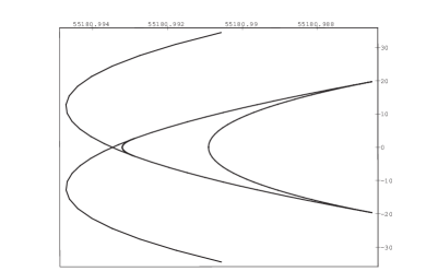
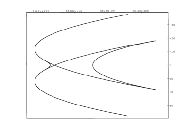
Figure 6: Typical “goblet” wavefront in the very late regime (in this case, $T=T_{l}+55000$). The middle-top panels shows a magnification of the throat. The middle-bottom and bottom panels show vertical and horizontal slices, respectively.

The last regime comprises all the wavefronts later than the critical time at which the inner “lips” merge with the outer “lips.” All such late wavefronts have a “regular” cuspidal ridge delimiting a concave surface that faces the observer, namely, a cuspidal ridge which is smooth as a curve in three space. Behind the foremost concave cap, the wavefront self-intersects and has another cuspidal ridge with four singular points in the general shape of an astroid or diamond. One such wavefront at time $T=T_{l}+10900$ is shown in Figure 5. In this front view, the foremost oval cuspidal ridge is clearly distinguishable, as are the two swallowtails in the back. However, there are two other swallowtails completing the diamond, which lie behind the foremost oval cap and are blocked from view in this picture. The qualitative structure of the wavefront in the diamond-ridge neighborhood is shown in the bottom panel of Figure 6.

A very late wavefront at time $T=T_{l}+55000$ is shown in Figure 6. It can be seen that as time moves on, the oval and diamond cuspidal ridges remain essentially unchanged except that the oval ridge in the foreground grows at a much faster rate than the diamond-shaped ridge in the back, and the wavefront eventually acquires a shape resembling that of a goblet. The figure shows both a field view of the “goblet” and a magnification of the goblet’s throat to show the diamond ridge. The diamond ridge structure is almost ubiquitous in wavefront evolutions that are not axi-symmetric. For another view of one of these local diamond ridges in wavefronts, we refer the reader to the bottom panel of Figure 10. The global “goblet” wavefront is typical of spherically symmetric regular potentials, with the major difference that the throat of the goblets in the spherically symmetric case degenerates down to a single point, lacking the complicated diamond structure for the case of elliptical symmetry. The diamond ridge represents the nondegenerate version of the throat of the goblet. The goblet’s throat has three wavefront sheets, each generically giving rise to an image of the light source.

What we have described in this section are precisely the singularities and metamorphosis of wavefronts in the observer’s lightcone in the case of an elliptical potential. In this case, we found that the wavefronts have three types of singularities: cuspidal ridges, swallowtail points, and points of transversal self-intersections. These three singularity types are shared by generic wavefronts in space — see p. 55 of Arnold (1991). We also showed that two kinds of metamorphosis occur for the wavefronts due to an elliptical potential. In the first place, we have found two occurrences of the birth of “lips” on the wavefront. Secondly, we have found two hyperbolic umbilic metamorphoses, i.e, the two symmetrical occurrences on the wavefront of the exchange of a swallowtail point from one cuspidal ridge to another. Both metamorphosis are part of Arnold’s list of metamorphoses of fronts in space — see, for instance, the first and fourth perestroikas in Figure 258 on page 489 of Arnold (1989).

VI.1.2 Caustic Sheet

If we think of the family of wavefronts for all times $T$ as spatial slices of the observer’s lightcone, then the collection of all the caustic singularities (i.e., cuspidal ridges, swallowtail points) on the instantaneous wavefronts forms a two-surface in spacetime. The projection of this two-surface into the comoving space $E$ is referred to as a comoving caustic surface.

As a surface in the three-space $E$, the caustic surface is traced in time by the caustics of the traveling wavefront as the front moves away from the observer. The metamorphoses of the wavefront’s caustics thus build up a picture of the caustic surface’s singularities. The generic singularities of a caustic surface in three-space are of five different types: folds, cuspidal ridges, swallowtail points, elliptic umbilic points and hyperbolic umbilic points Arnold (1986).

We showed that the caustic surface on an observer’s lightcone is given by equation (65). In the particular case of the elliptical potential, the resulting caustic surface is shown in Figure 7. A significant feature of our caustic surface in three-space is that it consists of two separate intersecting sheets, one for each non-trivial root (IV) of the Jacobian determinant in (IV). The two bottom panels in the figure show the two component sheets. One sheet starts closer to the observer as a horizontal “beak” and then develops a diamond cross section. The second sheet starts inside the first one as a vertical “beak” and eventually opens up into a smooth surface with an oval cross section. The transitions of both sheets take place at the points where they intersect. The points of intersection where the vertical beak disappears from the second component sheet and the vertical cusp ridge appears on the first component sheet are hyperbolic umbilic points — there are two such points.

We can also at this point give the exact value of the time of the first singular wavefront. This is the smaller of $T({\mbox{\boldmath$s$}}_{+}({\bf 0}),z_{+}({\bf 0}))$ and $T({\mbox{\boldmath$s$}}_{-}({\bf 0}),z_{-}({\bf 0}))$ since rays passing through the origin have the longest delay (as is evidenced from the spike). For the previous subsubsection, we have $T({\mbox{\boldmath$s$}}_{+}({\bf 0}),z_{+}({\bf 0}))=T_{l}+9699.27$ and $T({\mbox{\boldmath$s$}}_{-}({\bf 0}),z_{-}({\bf 0}))=T_{l}+10148.84$, i.e., the first singular wavefront is the surface at $T=T_{l}+9699.27$, as anticipated.

By slicing the caustic sheet with constant-$z$ surfaces we obtain a series of planar caustics representing the metamorphosis of the hyperbolic umbilic. These are shown in Figure 8 and coincide with the well-known caustic curves in the gravitational lensing literature for an elliptical potential — e.g., p. 386 of Petters et al. (2001). Beautiful photographs of caustic metamorphoses are shown in Nye (1999) — see p. 68 for the hyperbolic umbilic metamorphosis.

VI.2 Singular Elliptical Potential Lens

We shall illustrate the wavefront singularities and caustic surface due to a singular elliptical potential, namely, the case of vanishing core radius ($r_{c}=0$). In this case, it is simpler to use polar coordinates $(r,\vartheta)$ on the lens plane. We have for the potential,

$$\hat{\Psi}_{ep}^{sing}(r,\vartheta) \equiv A_{0}\sqrt{(1-\epsilon)r_{1}^{2}+(1+\epsilon)r_{2}^{2}}$$

$$= A_{0}\ r\sqrt{1+\epsilon\cos(2\vartheta)},$$

and for the associated bending angle,

$$\hat{{\mbox{\boldmath$\alpha$}}}_{ep}^{sing}(r,\vartheta)=\frac{A_{0}}{\sqrt{1+\epsilon\cos(2\vartheta)}}\Big{(}(1\!+\!\epsilon)\cos\vartheta,(1\!-\epsilon)\sin\vartheta\Big{)},$$

which has no dependence on $r$. The potential vanishes at the origin $r=0$. This case is singular because the surface mass density associated with the potential blows up at the origin of the lens plane (i.e., $\nabla^{2}_{\mbox{\boldmath$r$}}\hat{\Psi}_{ep}^{sing}({\mbox{\boldmath$r$}})\rightarrow\infty$ as ${\mbox{\boldmath$r$}}\rightarrow{\bf 0}$). The center of the lens (i.e., the origin) thus acts as an obstruction to the light rays — see Petters (1995)) and p. 544 of Petters et al. (2001) for a detailed treatment of obstruction points. Soon after going through the lens plane, the wavefronts evolve markedly differently from the nonsingular case. For our illustrations, we have used the following values of the lens parameters: $A_{0}=0.3,\epsilon=0.02,z_{l}=4000$. As in the regular case, these values are chosen for pedagogical reasons, although taking care to respect the approximations of small angles.

VI.2.1 Wavefront Singularities

Due to the obstruction at the center of the lens (i.e., the origin), all the wavefronts are singular and there are only two regimes. The first regime consists entirely of a single wavefront (the earliest one to make it past the lens plane) with an interior spike pointing towards the observer, as did the wavefronts of the nonsingular elliptical potential. However, in this singular case the spike is conical, and touches the lens plane at the origin. The point at the tip of the spike is removed. This wavefront, $T=T_{l}=4000$, is shown in Figure 9. The figure shows both a field view of the wavefront, and a side view of the tip of the spike magnified to make the conical character apparent.

At all times afterwards, the wavefronts resemble a goblet — the second regime. However, these goblets are markedly different from those that resulted at late times in the nonsingular elliptical potential case. There is a single diamond-shaped cuspidal ridge, which lies at the throat of the goblet. The rim of the goblet is removed and acts as a boundary of the wavefront. These goblets lack the interior concave surface facing the observer that characterizes the goblets in the nonsingular case. The throat of the goblet has three sheets, each typically giving rise to an image of the source. One such wavefront in this regime ($T=T_{l}+1000$) is illustrated in Figure 10, where a field view evidences the resemblance to a goblet. The bottom panel in the figure shows a magnified view of the throat of the “goblet” where the diamond structure is evident.

Two questions relating to this imperfect “goblet” wavefront arise. In the first place, do the wavefronts ever detach from the lens plane, or, on the contrary, do they reach out to the obstruction point? As one can appreciate in Figure 11, where a given portion of the initial wavefront at $T=T_{l}$ is followed up and plotted again at $T=T_{l}+1000$, the wavefront does not remain attached to the lens plane.

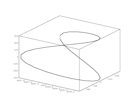
Figure 12: The boundary of the wavefront in the critical case. Middle and bottom panels show side and front views.

The second question is whether the rim of the goblet is planar, namely, whether it lies on a constant-$z$ plane. The answer is no. The rim of the goblet is a space curve, which is plotted in Figure 12. It must be kept in mind that the rim is the boundary of the wavefront. This rim is removed because it is the image of the point $r=0$ on the lens plane under the wavefront lensing map, i.e., ${\mbox{\boldmath$w$}}_{T,ep}^{sing}(0,\vartheta)=({\mbox{\boldmath$s$}}(0,\vartheta,T),z(0,\vartheta,T))$, which is a space curve for fixed $T$. Explicitly, equations (32) and (33) yield that

$${\mbox{\boldmath$s$}}(0,\vartheta,T) = \frac{-\left(T\ +\ z_{l}\ |\hat{{\mbox{\boldmath$\alpha$}}}_{ep}^{sing}(\vartheta)|^{2}/2\right)\hat{{\mbox{\boldmath$\alpha$}}}_{ep}^{sing}(\vartheta)}{\displaystyle 1\ +\ |\hat{{\mbox{\boldmath$\alpha$}}}_{ep}^{sing}(\vartheta)|^{2}/2}$$

$$\hskip 108.405pt+\ z_{l}\ \hat{{\mbox{\boldmath$\alpha$}}}_{ep}^{sing}(\vartheta),$$

$$z(0,\vartheta,T) = \frac{T\ +\ z_{l}\ |\hat{{\mbox{\boldmath$\alpha$}}}_{ep}^{sing}(\vartheta)|^{2}/2}{1\ +\ |\hat{{\mbox{\boldmath$\alpha$}}}_{ep}^{sing}(\vartheta)|^{2}/2}.$$

As is seen from these equations, the ultimate reason why the wavefronts have a whole elliptical curve’s worth of boundary points instead of only one point is that the bending angle vector field $\hat{{\mbox{\boldmath$\alpha$}}}_{ep}^{sing}$ does not depend on $r$.

In rectangular coordinates, the map $\hat{{\mbox{\boldmath$\alpha$}}}_{ep}^{sing}$ is ill-defined at the origin ${\mbox{\boldmath$r$}}={\bf 0}$. It has a singularity of the type 0/0 since

$$\hat{{\mbox{\boldmath$\alpha$}}}_{ep}^{sing}({\mbox{\boldmath$r$}})=\frac{A_{0}^{2}\Big{(}(1-\epsilon)r_{1},(1+\epsilon)r_{2}\Big{)}}{\hat{\Psi}_{ep}^{sing}({\mbox{\boldmath$r$}})}.$$

One can approach the singular point from different directions in the lens plane and hope that the limit would be the same in all directions. However, the limiting value of the $\hat{{\mbox{\boldmath$\alpha$}}}_{ep}^{sing}({\mbox{\boldmath$r$}})$ as ${\mbox{\boldmath$r$}}\to{\bf 0}$ is direction-dependent, as signaled by the direction-dependent bending angle $\vartheta$ in (VI.2.1). In this atypically singular case, obstructing one light ray (the one that passes through the center of the lens) removes an elliptical curve’s worth of points on the wavefront. If a source is outside the rim, then one lensed image is seen of the source, while two images are seen if the source is inside the rim. This phenomenon seems to have been first noted on p. 188 of Petters et al. (2001) for the case of a singular isothermal sphere (i.e., $r_{c}=\epsilon=0$), where the rim is a circle, as discussed in Subsection VI.3

VI.2.2 Caustic Sheet

The caustic sheet in this case is obtained by the same method as in the case of a nonsingular elliptical potential. The use of polar coordinates $(r,\vartheta)$ simplifies the calculation. We have

$$\mathop{\rm det}\nolimits\frac{\partial{\mbox{\boldmath$s$}}_{z}}{\partial{\mbox{\boldmath$r$}}} = \cos(2\vartheta)\ \mathop{\rm det}\nolimits\frac{\partial{\mbox{\boldmath$s$}}_{z}({\mbox{\boldmath$r$}})}{\partial(r,\vartheta)}$$

$$= \cos(2\phi)\left(\frac{\partial x}{\partial r}\frac{\partial y}{\partial\vartheta}-\frac{\partial x}{\partial\vartheta}\frac{\partial y}{\partial r}\right),$$

where $x$ and $y$ are the cartesian components of the lensing map ${\mbox{\boldmath$s$}}_{z}$. In this case, the components reduce to

$$x = \left(\frac{z}{z_{l}}\ r-\frac{(z-z_{l})A_{0}(1+\epsilon)}{\sqrt{1+\epsilon\cos(2\vartheta)}}\right)\cos\vartheta,$$

$$y = \left(\frac{z}{z_{l}}\ r-\frac{(z-z_{l})A_{0}(1-\epsilon)}{\sqrt{1+\epsilon\cos(2\vartheta)}}\right)\sin\vartheta,$$

and the vanishing of the Jacobian determinant — see equation (IV) — becomes

$$0 = \mathop{\rm det}\nolimits\frac{\partial{\mbox{\boldmath$s$}}_{z}}{\partial{\mbox{\boldmath$r$}}}=\frac{z\cos(2\vartheta)}{z_{l}(1\!+\!\epsilon\cos(2\vartheta))^{\frac{3}{2}}}\Big{[}z\Big{(}(1\!+\!\epsilon\cos(2\vartheta))^{\frac{3}{2}}\frac{r}{z_{l}}$$

$$\hskip 86.72377pt-\ A_{0}(1\!-\!\epsilon^{2})\Big{)}\ +\ z_{l}A_{0}(1\!-\!\epsilon^{2})\Big{]}.$$

The unphysical root $z=0$, which defines the plane of the observer, is responsible for the absence of a second component caustic sheet, the most notable aspect of the caustic sheet in the singular case. The (one component) caustic sheet is obtained from the non-trivial root, i.e.,

$$z=z_{c}(r,\vartheta)\equiv-\frac{z_{l}A_{0}(1-\epsilon^{2})}{(1+\epsilon\cos(2\vartheta))^{\frac{3}{2}}\ r/z_{l}-A_{0}(1-\epsilon^{2})}.$$ (73)

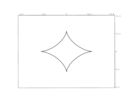
Figure 14: Typical planar caustic in the singular case.

A plot of the caustic sheet is shown in Figure 13. The surface has four cuspidal ridges with a conical profile, which can clearly be appreciated in the bottom panel of the figure. The tip of the caustic surface lies at the center of the lens (origin) and is removed. Slicing the caustic sheet with constant$-z$ planes we obtain the $z$-planar caustic curves. The planar caustics are astroid-shaped curves with four cusps, as can be seen in Figure 14. A source inside the caustic curve has four lensed images, while a source outside has two.

VI.2.3 Caustic Surfing

The singular elliptical potential provides an excellent opportunity to illustrate the caustic surfing scheme. We start by pointing out that the caustic sheet, which is parametrically given by (VI.2.2) and (73), can equivalently be given by the following expression:

$$S_{0}({\sf x})\equiv\left((1+\epsilon)x^{2}\right)^{\frac{1}{3}}+\left((1-\epsilon)y^{2}\right)^{\frac{1}{3}}-\left(2\epsilon A_{0}(z-z_{l})\right)^{\frac{2}{3}}=0$$

This expression assumes that the apex of the lightcone where the caustic lies is at the origin of coordinates, and the lens plane is at a distance $z_{l}$ from it.

Suppose now that a source is moving on the light source plane with an approximately constant velocity ${\sf V}=(V_{1},V_{2},0)$, carrying its own lightcone with it. Then the caustic on the source’s lightcone moves as well, and at any given instant of conformal time ${\sf t}$, assuming the motion is sufficiently slow, the caustic surface can be given as $S({\sf x},{\sf t})=S_{0}({\sf x}-{\sf V}{\sf t})$. Assume that a space-borne telescope observes at time ${\sf t}=0$ an image of the source at peak magnification. ¿From the location of the image, by the (comoving) lens map we can determine the location $s$ of the source on the source plane. But for our purposes we need to switch the point of view and think of the lightcone of the source instead: The source lies at the origin and the telescope at a location $(x_{0},y_{0},z_{0})=(-{\mbox{\boldmath$s$}}\ell_{tl}/\ell_{sl},\ell_{tl}+\ell_{sl}),$ where $\ell_{tl}$ and $\ell_{sl}$ are the distance between the telescope and the lens plane, and between the lens plane and the source plane, resp. Because $(x_{0},y_{0},z_{0})$ lies on the comoving future caustic sheet of the source at ${\sf t}=0$, we have

$$S_{0}({\sf x}_{0})=0=\left((1+\epsilon)x_{0}^{2}\right)^{\frac{1}{3}}+\left((1-\epsilon)y_{0}^{2}\right)^{\frac{1}{3}}-\left(2\epsilon A_{0}\ell_{tl}\right)^{\frac{2}{3}},$$ (74)

where we have made the substitution $z_{l}=\ell_{tl}$. Now, we calculate the speed ${\sf v}_{min}$ that the telescope needs to stay on the caustic sheet during the time increment $\delta{\sf t}.$ ¿From our discussion in Section V, specifically Eq. (69), we have

$${\sf v}_{min} = \frac{V_{1}\left[(1+\epsilon)/x_{0}\right]^{\frac{1}{3}}+V_{2}\left[(1-\epsilon)/y_{0}\right]^{\frac{1}{3}}}{\left[(1+\epsilon)/x_{0}\right]^{\frac{2}{3}}+\left[(1-\epsilon)/y_{0}\right]^{\frac{2}{3}}+\left[4\epsilon^{2}A_{0}^{2}/\ell_{tl}\right]^{\frac{2}{3}}}\times$$

$$\hskip 21.68121pt\left(\left(\frac{1+\epsilon}{x_{0}}\right)^{\frac{1}{3}},\left(\frac{1-\epsilon}{y_{0}}\right)^{\frac{1}{3}},-\left(\frac{4\epsilon^{2}A_{0}^{2}}{\ell_{tl}}\right)^{\frac{1}{3}}\right)$$

In this expression, all the symbols are known in principle. The values of $x_{0}$ and $y_{0}$ can be found via the lens mapping at the observation event, as explained above. Clearly, this may be a technically complex procedure, considering that it is only a first step in a iterative scheme to place the telescope on the caustic sheet. Our main purpose is to show that the calculation is feasible in principle.

VI.3 Singular Isothermal Sphere Lens

For a singular isothermal sphere lens, we have $r_{c}=\epsilon=0$. The potential and bending angle vector are given respectively as follows:

$$\hat{\Psi}_{ep}^{sis}(r,\vartheta)=A_{0}\ r,\qquad\hat{{\mbox{\boldmath$\alpha$}}}_{ep}^{sis}(r,\vartheta)=A_{0}(\cos\vartheta,\sin\vartheta).$$

The wavefronts are similar to those of the singular elliptical potential, except that the throat of the goblet is a point and the singular rim of the goblet is a circle — see Figure 15. The caustic surface collapses to a line coinciding with the portion of the optical axis beyond the lens plane (i.e., $z>z_{l}$). Note the origin on the lens plane, which is a singularity of the lens, is not a part of the caustic line. We have that each $z$-planar caustic is a point.

VII Concluding remarks and outlook

We have shown how to construct a lensing map that takes points on the lens plane into points on a wavefront surface, as opposed to a source plane. This represents a sort of “instantaneous” lens map, carrying a sense of constant time. By contrast, the standard lens map carries no sense of time at all. Additionally, the wavefront lensing map has an asymmetric Jacobian matrix. Notice that, barring multiple sheets, the wavefront surface lies very close to a plane in the weak-field case, as illustrated in most of our figures. In the figures the optical axis is magnified several times in order to appreciate the distance between the different sheets in the folded wavefront. Our intial motivation for explicitly constructing a wavefront-lens mapping was inspired by several works (e.g., Berry and Upstill (1980); Nityananda (1990); Petters (1993); Frittelli and Newman (1999); Ehlers et al. (2002)). In this respect, it appears that an extension of our constructions in Secs. III and IV beyond the weak field domain is feasible Ehlers (2000); Perlick (2001).

We took advantage of the conformally flat nature of the flat FL universe in order to make use of a comoving lens equation, which in addition to being comoving is also a conformal lens equation. A conformally related flat spacetime exists, of course, in all three types of FL universes, so in principle, our wavefront map could be adapted for interpretation in the open or closed universes. However, in such universes the conformal factor relating the FL universes to the corresponding flat spacetime depends on the space point, as well as the time, and the translation of our conformal present proper length function to a cosmological present proper length is not at all as direct as we found it in this work. Some of the subtleties that would be involved in the translation in the open and closed cases are treated in detail by Frittelli, Kling and Newman Frittelli et al. , where the conformally flat lens map and time delay are transformed into the cosmological lensing map and time delay. Nonetheless, we do not need to rely on the conformally related flat space to calculate our present proper length function.

The individual wavefronts for the potentials illustrated proved useful in visualizing the relationship between the location of the source in reference to the caustic, and the number of images observed. Additionally, the wavefronts of the singular potentials helped explain the anomalous counting of images observed by Petters, Levine, and Wambsganss Petters et al. (2001), p. 188. The latter showed that in the case of the singular potentials there is a simple closed curve, that is not a caustic, but that separates regions in the source plane where the number of images differs by one, rather than two. We have here shown that such a curve is the boundary of the wavefront, it is not a caustic, and the number of images differs by one less than in the regular case because one whole sheet of the wavefront is missing due to an obstruction in the lens plane.

Lastly, we have taken a step towards a preliminary scheme for caustic surfing in a meaningful and consistent manner. The form of the subsequent iterations remains an open problem, as does the implementation of the procedure, particularly the measurement of the transverse velocity of the the moving source that one intends to follow. Clearly the caustic surfing proposal depends only on the caustic surface, and not on the method used to obtain it. But the point is that optimal caustic surfing (with the least effort) is achieved only by allowing the telescope to surf the caustic sheet, rather than the planar caustics at fixed distance from the source. One could also image scenarios where a telescope may not ride a caustic sheet, but move so as to stay inside certain chambers of the caustic surface (compare with Gaudi and Gould Gould and Gaudi (1997)), possibly near higher order singularities. Future studies of the aforementioned issues are clearly warranted.

Figure 1: A portion of the wavefront of an elliptical potential in the regular regime, i.e., early times past the lens plane (in this case, $T=T_{l}+8900$). The observer is to the right at $(0,0,0)$.

Figure 2: The single lips regime ($T=T_{l}+9800$). The bottom panel shows a front view of the lips singularity.

Figure 3: Typical wavefront in the criss-cross lip regime ($T=T_{l}+10200$), where two nested perpendicular cuspidal ridges are present. The middle panel is a vertical slice of the top panel, while the bottom panel is a horizontal slice. Both slices are through the optical axis.

Figure 4: The critical wavefront ($T=T_{l}+10420$).

Figure 5: Typical wavefront early in the late regime ($T=T_{l}+10900$). The bottom panel shows a front view.

Figure 7: Caustic sheet of the elliptical potential. The two component sheets are represented separately in the middle and bottom panels.

Figure 8: The metamorphosis of the planar caustics arising from $z$-plane slices of the caustic surface.

Figure 9: The unique wavefront in the early regime ($T=T_{l}$) in the singular case. The bottom panel shows a side view of the tip of the spike.

Figure 10: Typical wavefront in the late regime ($T=T_{l}+1000$) in the singular case. The bottom panel shows a magnified view of the “throat” of the goblet.

Figure 11: Progression of a portion of the wavefront in the singular case. The observer is on the right.

Figure 13: The caustic sheet in the singular case

Figure 15: Wavefront due to a singular isothermal sphere. The top panel shows a field view, and the bottom panel shows a slice or profile of the wavefront. Notice that the wavefront is a surface of revolution around the optical axis.