Abstract

It is now ten years since the first microquasar GRS 1915+105 was discovered. More than six years of observations with RossiXTE have shown a level of variability never observed in any other X-ray source. Here I try to address some issues, based on X-ray observations only, that have relevance for theoretical modeling. First, I ignore these peculiarities and concentrate on the similarities with other X-ray transients. Then I focus on the peculiar variability and present a number of obervational facts that need to be addressed by theoretical models.

1 GRS 1915+105 from GRANAT to RossiXTE

As practically all articles about GRS 1915+105 start, the source was discovered ten years ago, in 1992, with the Watch instrument on board GRANAT [1]. Figure 1 shows the original discovery light curve from that work, where one can see that the source was very variable from the beginning. As a comparison, the full RossiXTE/ASM light curve up to 2002 July is shown in the bottom panel of Fig. 1. Already from these plots, it is evident that the variability of GRS 1915+105 is rather unique and that in this source we are observing something which is not observed in other sources.

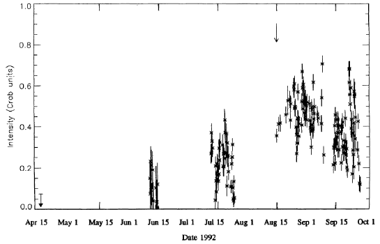
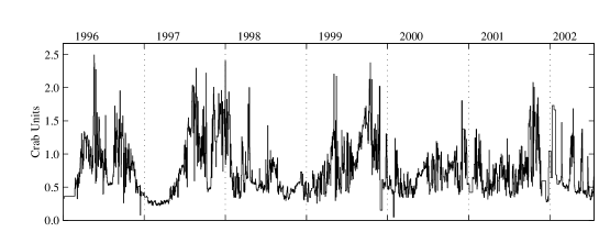
Figure 1.: GRS 1915+105 long-term light curves. Top: GRANAT/Watch [1]. Bottom: RossiXTE/ASM up to 2002 July 19.

When examining the variability at shorter time scales, as observed with the RossiXTE/PCA, things become even more complex (see Fig. 2), showing a definite structure, which in this particular case repeats almost unchanged after about 25 minutes. The complexity of these light curves, first shown by [2], is analyzed and categorized by [3], who classify the light curves in a dozen variability classes and identify three basic spectral states called A, B and C. In these ten years, many papers have been devoted to the analysis and interpretation of the X-ray observations of GRS 1915+105, and it is not possible to review them all here. What I want to do is to put this unique source in perspective, comparing it with other transient BHCs. First, I will emphasize the similarities with other systems, then I will concentrate on the peculiarities.

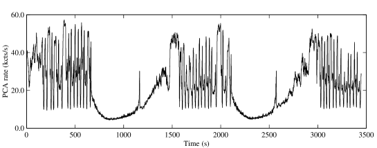
Figure 2.: Example of a RossiXTE/PCA light curve of GRS 1915+105, from 1997 October 31.

2 GRS 1915+105 as a transient

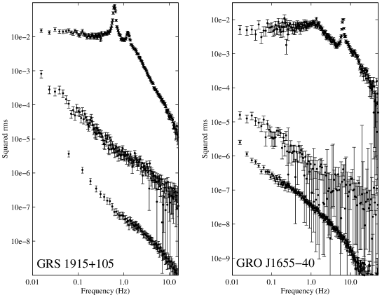
Figure 3.: Left panel: PDS of the three basic spectral states of GRS 1915+105 (C, A and B from top to bottom, shifted by a factor of 100 from each other). Right panel: PDS of three observations from the latest stages of the outburst of GRO J1655-40, shifted in the same way.

Looking at GRS 1915+105 as an X-ray transient, if we ignore the most obvious peculiarities, we can identify some common features which the system shares with all other BH systems. One is the shape of the Power Density Spectra (PDS) above, say, 1 Hertz (see e.g. [4, 5]). A second one is the shape of the broad-band energy spectra as observed with BeppoSAX and RossiXTE: the presence of a soft thermal component plus a hard component that at times can extend to very high energies (see e.g. [6, 7, 8, 9]).

In order to compare the shape of the PDS, let us consider three representative cases, corresponding to time intervals when the source is not wildly variable as in Fig. 2, corresponding to the A, B and C states identified by [3] (Fig 3, left panel). They can be compared to the PDS observed from the microquasar GRO J1655-40, which are typical from the so-called canonical states of BHC [10]. One can see that the similarities are rather strong, indicating a connection between the states of GRS 1915+105 and the “canonical” states of other BHCs. A more detailed analysis is presented in [11].

Turning to the energy spectra, a comparison based on X-ray colors is also considered in [11]. However, more interesting here is to notice that the 1-10 Hz QPO observed in the C state of GRS 1915+105 follows the same correlation with the slope of the power-law component in the energy spectrum which is observed in a number of other sources [12]. The correlation can be see in Fig. 4 for GRS 1915+105 and for the bright transient XTE J1550-564. Also in this case there are striking similarities, including the indication of a turnoff of the relation at high QPO frequencies.

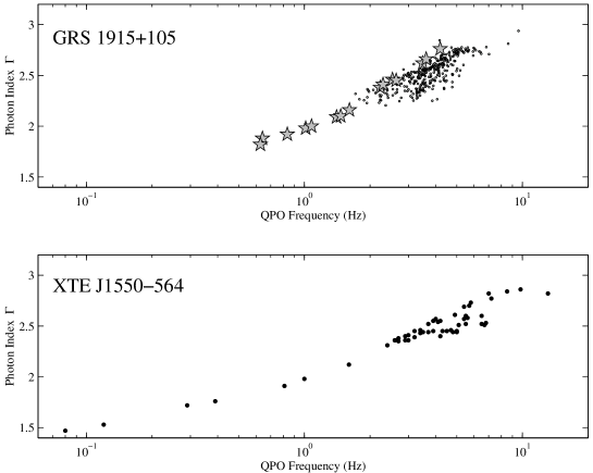
Figure 4.: Top panel: QPO-$\Gamma$ correlation for selected C state intervals of GRS 1915+105 (stars indicate $\chi$-class observations). Bottom panel: the same correlation observed in XTE J1550-564.

All this indicates that, when ignoring intervals of strong and peculiar variability, GRS 1915+105 behaves in a rather similar way to other transient systems and, if these were the only available data, would be indistinguishable from them.

3 GRS 1915+105 as a peculiar source

Of course it is not really possible to ignore the most interesting parts of the observations of this source. Therefore, let’s turn to the peculiarities of GRS 1915+105 and consider what we can learn from it. The observed oscillations in flux and energy spectrum, occurring on time scales from a few minutes to months, have been interpreted as due to the onset of an instability which causes the innermost region of the accretion disk to switch between a visible and a non-visible state [6, 7]. This idea has been recently developed theoretically by a number of authors, who tried to reproduce the observed light curves with some success [15, 16, 17, 18]. However, only the most basic features of the observations are taken into account by these works.

A more detailed observational approach has been followed by [8], who analyzed a large number of spectra of GRS 1915+105 and presented correlation between timing and spectral parameters. Recently, a complete analysis of a large number of RossiXTE/PCA observations, with the production of energy spectra on the time scale of 16 seconds, has been presented by [19]. An example of this analysis is shown in Fig. 5, where an observation interval is shown, together with the time history of the spectral parameters. A clear evolution in spectral parameters is observed. These parameters can be correlated with each other and can give important clues to detailed theoretical models as those mentioned above. An important example is shown in Fig. 6. Here the best-fit inner radius and temperature of the accretion disk are plotted versus each other (notice that although the absolute value of the inner disk cannot be taken at face value, its variations are a more solid measurement [13]).The points, corresponding to different $\chi$ (state C only) observations, follow a power-law correlation with index $\alpha\sim-$0.4, much flatter than the value $\alpha=-3/4$ expected from a Shakura & Sunyaev disk at constant mass accretion rate. This indicates that moving from large radii to smaller radii, the measured local accretion rate through the disk at that radius decreases. The possible association of this decrease in local accretion rate and the generation of jets should be considered.

Figure 5.: Time evolution of spectral parameters of an observation interval of GRS 1915+105 as observed by the RossiXTE/PCA. Panels are (top to bottom): PCA light curve, power-law photon index $\Gamma$, disk inner temperature and radius, flux of the power-law and the of the disk component.

Figure 6.: Correlation between inner disk temperature and radius for a selected subsample of C-state intervals of GRS 1915+105 observed by RossiXTE/PCA. Time resolution is 16 seconds.

To put these variations in a broader perspective, we can expand the plot of Fig. 6 and include the corresponding state-A and state-B intervals. This is done in Fig. 7, where also two lines at constant mass accretion rate are plotted. In addition to the $\alpha\sim-$0.4 described before for state C (notice that this branch is followed twice, in opposite directions), we can see that as the radius decreases further (state A), the points follow precisely a $\alpha=-3/4$ correlation, indicating that here the local mass accretion rate is indeed constant. Notice that the soft state A takes place after the radio event starts, indicating that state A comes after a jet emission [14]. After state A, the source enters state B, where the radius has reached its minimum value and the temperature slowly increases, thereby increasing again the local mass accretion rate (see also [6, 3]). Once again, the behavior shown in Fig. 7 needs to be addressed together with the shape of the light curves by any theoretical model that aims at the interpretation of the peculiarities of GRS 1915+105.

4 The biggest challenges

As I have shown in the previous sections, there are a number of detailed observational results that can provide inputs to theoretical models for the understanding of GRS 1915+105, and for connecting them to what is observed from other BHCs. In this last section I would like to show two of the most outstanding features of this source, features which I consider as the biggest challenges for any theoretical model to be applied to the peculiarities of this source. The first is the presence of extreme variability on time scales down to 0.2 seconds (see Fig. 8, top panel). This variability is accompanied by changes in the X-ray colors, i.e. the spectrum softens when the flux decreases [3]. These changes can be attributed to changes in the temperature of the inner disk, and therefore to variations in the local mass accretion rate. This can happen on a local viscous time scale, which is in the observed range. The cause of this variability, spectrally different from the disk oscillations commonly considered, needs to be understood.

Figure 7.: Same as Fig. 6, but including the corresponding A-state and B-state intervals. The two diagonal lines correspond to lines of constant mass accretion rate for a Shakura & Sunyaev disk.

The second challenge is the extreme degree of similarity between light curves (and corresponding spectral evolution) of observations from different variability classes (see [3]). The dozen pattern that have been identified in the light curves of GRS 1915+105 might seem many, but in reality they are surprisingly few, considering all possibilities for the oscillations. The fact that the source locks itself in this relatively small set of patterns might be a key for the understanding of the origin of the variability. Moreover, not only the general shape of the light curve, but also specific details can be found in observations years apart. As an example (from [20]), in the bottom panels of Fig. 8 I show two light curves well distant in time where the pattern of variability is followed even to some (albeit not all) details. Notice that one of the two light curves (the top one) has been rescaled in time in order to match the time scale of the other, indicating that some time scale underlying the whole process must have been different. Of course it is not realistic to ask for a theoretical model that explains and reproduces the exact shape of the light curves in Fig. 8. However, the simple fact that such complex shapes are in some way characteristic of the system should be taken into account when developing models. For instance, models like that of [18], which produce encouraging light curves, should as a next step keep into account more details of the observations (like those in Fig. 8) without running the risk of trying to interpret noise in the system.

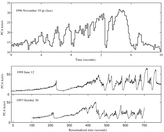
Figure 8.: Top panel: PCA light curve from a $\rho$-class observation with 1/8 s binning. Very large-amplitude and fast variability is evident. Bottom panels: two PCA light curves (1s binning) from almost two years apart. The topmost one has been rescaled in time to highlight similarities in the shape.

5 Conclusions

GRS 1915+105 is a peculiar black-hole transient in at least two ways. First, it can hardly be considered a transient, since it is in “outburst” since ten years at large values of the accretion rate. Second, as shown before, the variability of its flux and spectral properties are unique and extremely complex. However, not all its properties are unique (as in the case of XTE J0421+56, see [21, 22, 23]), indicating that we are not dealing with a source completely different from the others. This can be turned to our advantage: by linking “normal” and peculiar characteristics, we can learn something general about accretion onto black holes.