An Empirical Model for the Radio Emission from Pulsars

Abstract

A pulsar model is proposed which involves the entire magnetosphere in the production of the observed coherent radio emission. The observationally-inferred regularity of peaks in the pulsar profiles of ‘slow’ pulsars (Rankin 1990,1993a), is shown to suggest that inner and outer cones of emission near the polar cap interact with and ‘mirror’ two rings in the outer magnetosphere: one where the null line intersects the light-cylinder, and another where it intersects the boundary of the corotating dead zone. The observed dependency of conal type on period is shown to follow naturally from the assumption that cones only form when the mirror intersection points lie between two fixed heights from the surface, suggesting that a feedback system exists between the surface and the mirror points, accomplished by a flow of charges of opposite sign in either direction. In their flow to and from the mirror points, the particles execute an azimuthal drift around the magnetic pole, thereby creating a ring of discrete ‘emission nodes’ close to the surface. Motion of the nodes is observed as subpulse ‘drift’, which is interpreted here as a small residual component of the real particle drift. The nodes can move in either direction or even remain stationary, and can differ in the inner and outer cones. A precise fit is found for the drifting subpulses of PSR0943+10. Azimuthal interactions between different regions of the magnetosphere depend on the angle between the magnetic and rotation axes and influence the conal type, as observed. The model sees ‘slow’ pulsars as being at the end of an evolutionary development where the outer gap region no longer produces pair cascades, but is still the intermittent source of low-energy pairs in a magnetosphere-wide feedback system.

1 INTRODUCTION

In 1975 Ruderman $\&$ Sutherland (henceforth RS) proposed a model for pulsar emission which postulated a gap region located immediately above the neutron star surface and, as a result of the inability of the electric field to remove ions from the surface, subject to an intense potential difference of around $10^{14}eV$. In this gap pair-production in the intense magnetic field generated electrons which heated the surface and created localised discharging regions. These ‘sparks’ drifted around the magnetic pole and ejected energetic particles into the magnetosphere where a bunching mechanism, first proposed by Sturrock (1971), created coherent radiation following a two-stream instability. The model has been highly influential, since it provides a quantitative framework within which theorists and observers can work, and one of its underlying tenets, that the sources of pulsar radio emission are plasma columns circulating just above the polar cap, is now widely accepted.

Nevertheless, over the years the polar gap model has been questioned on theoretical grounds, largely through difficulties with the neutron star surface binding energy (e.g. Jones 1985, 1986, Abraham $\&$ Shapiro, 1991, Neuhauser et al, 1987) and with the high plasma densities required in the emisson regions (Lesch et al, 1998). On observational grounds too it is not easy to reconcile the model with the complexity of subpulse behaviour, such as stationary or counter-drifting subpulses (e.g. Biggs et al. 1985, Nowakowski 1991), mode changing and nulling. Evidence that the emission profiles generally take the form of nested cones (Rankin 1983, Lyne $\&$ Manchester 1988, Rankin 1990(RI), 1993a(RII), 1993b) has presented a further challenge to the model, and only by appealing to surface multipoles (e.g. Gil et al, 2002a,b) does it seem possible to confine the ‘sparks’ either radially or azimuthally. More recently, the precisely drifting emission columns of PSR0943+10, analysed in great detail by Deshpande $\&$ Rankin (1999, 2001 (henceforth DR)), convincingly confirm the picture of circulating plasma columns. However the observed circulation rate is only reconcilable with the RS model by adopting a potential difference across the cap which is significantly lower than that predicted by the RS model, and - if generated by surface magnetic features - the columns would seem to require multipoles with a high degree of regularity (Asseo $\&$ Khechinasvili 2001, Gil et al 2002a,b).

In response to these difficulties, some authors have analysed magnetospheres based on free electron flows from the polar cap and gradual acceleration into the upper magnetosphere (‘inner accelerator’ models) (e.g. Arons $\&$ Scharlemann 1979, Mestel $\&$ Shibata 1994, Hibschmann $\&$ Arons 2001a,b (henceforth HAa,b), Harding $\&$ Muslimov 2002 (HM), Harding et al 2002 (HMZ), Harding $\&$ Muslimov 2003). Such models are often part of wider attempts at creating a self-consistent global magnetosphere (Mestel et al 1985, Shibata 1995, Mestel 1999 and references therein). Although arguably more consistent with the physics of the neutron star surface - and with the overall current balance and torque transfer requirements - these models lack the predictive power of the RS model when faced with detailed radio observations. Possibly the belief prevails that radio emission, undoubtedly originating just a few tens of stellar radio above the surface and energetically weak compared to the spin-down energy loss, has little to say about global conditions. Furthermore the sheer complexity of highly time-dependent subpulse phenomena acts as a great deterrent to theoreticians seeking to define a steady state condition.

In trying to bring the large-scale magnetosphere models closer to observational testing, and in a deliberate attempt to explore the link between the the observed polar cap activity and the outer magnetosphere, we have taken a fresh look at the radio profiles analysed in RI and RII. Pulsar integrated profiles are suitable to this purpose, since they are one feature of pulsar observations which displays great stability: a pulsar’s profile is its invariant signature. Rankin’s conal classification of the profile forms is here interpreted essentially from a geometric standpoint without prejudice for or against any particular formation process. In essence, we seek to use the profiles as diagnostics of the magnetosphere’s structure.

This paper argues that if regular conal structures exist in all or most pulsar profiles - as claimed in RI and RII - then explanations in terms of complex polar magnetic field topology are difficult to support, since they would require similar magnetic topologies from pulsar to pulsar. However it is suggested here that conal emission may be the natural geometric result of interactions between the polar cap and outer regions of the outer magnetosphere in the purely dipolar environment of ‘slow‘ older pulsars, provided that the once prolific outergap production of pairs of a pulsar in its early life is now weak and intermittent. This proposed evolutionary link between the younger faster pulsars (such as the Crab pulsar), whose principle emission is in the gamma-ray band, and the older weaker radio pulsars is seen as a major and novel feature of the model here.

First, in section (2), it is argued that the fixed ratio of the cone radii is consistent with the assumption that emission occurs preferentially on two critical sets of field-lines, one bounding the corotating dead zone (defined by the last field-line to close within the light-cylinder), the other passing through the intersection of the null line (defined as the boundary between regions of net charge density of opposing sign) and the light cylinder. In section (3) it is shown that the observed period dependence of conal types can be simply explained if emission is possible only if a ‘mirror’ point (i.e. an intersection of the null line with the critical field-lines) lies between two fixed altitudes. In section (4) it is shown how the inevitable drift of the inflowing and outflowing particles about the magnetic axis causes ‘emission nodes’ to form above the surface, and, in section (5), that this leads to their precession around the magnetic pole, generating the well-known phenomenon of ‘drifting subpulses’ and hence the double cone structure. In section (6) the drift model is applied to the pulsar PSR0943+10 and precise fits to both the B-mode and the Q-mode are found. In section (7) the global nature of the pulsar phenomenon is stressed: azimuthal interactions between critical regions of the outer magnetosphere are shown to explain the observed dependency of conal formation on the angle of inclination. Finally, in section (8), the physical requirements of the underlying feedback system are discussed in the light of current physical ideas.

The sketched model which emerges from this analysis contains many elements of the RS model, but on a scale which involves the entire magnetosphere: particles (presumed here to be electrons, although the system is sign-reversible) are accelerated from low Lorentz factors close to the polar cap to achieve high $\gamma$ near the outer gap, which stretches from the corotating dead zone of the magnetosphere to the light cylinder. Pair creation occurs in these regions, although certainly not in the profusion of the pair cascades supposed in Crab-like pulsars (Cheng et al, 1986, Romani $\&$ Yadiaroglu, 1995). Rather the production is likely to be intermittent, weak (ie of low multiplicity with low Lorentz factors) and azimuthally-dependent, with most of the particles produced forming a wind beyond the light cylinder, but with a small but essential fraction of the positrons returning to the surface, accelerated and funnelled by the increasingly tight bundle of magnetic field-lines above the poles (Michel 1992).

Unlike the case of fast pulsars (Cheng et al, 1986), the downward flow of particles is inadequate to screen the polar potential. Shortly before reaching the surface, the positrons emit sufficiently energetic radiation to cause a bunched avalanche of pairs which bombard the surface with coherent radiation. This is then reflected and contributes to the core component of the pulsar profile. Residual electrons formed by this process (maybe augmented by electrons emitted from the heated spot on the surface) are then accelerated back to the outer gap. This process is then repeated, and is reinforced if the combined and equal drifts of the electrons and positrons around the pole maintain the hot spots at locations which are either fixed in azimuth or drift slowly backwards or forwards. The outflowing electrons are somehow stratified by the inflowing layers of pairs, and radiate curvature radiation parallel to the field lines and at about 200 km (for 1GHz) above the surface. The holistic nature of the model means that the radio emission can simply be seen as an image of, and as driven by, the activities of the outer gap.

The emission, particle flow and pair-creation processes are not worked out in detail here, and in many cases have been cannibalised from existing models (especially Mestel et al (1985), Michel (1992), Shibata (1994), HAa,b, HM, HMZ, Hirotani $\&$ Shibata 1999, 2001 (HSa,b)). Some features lack, as yet, a proper theoretical investigation: for example, the mechanism and level of weak low-energy pair production in outergaps has never been explored, since hitherto it has been assumed that outergaps only play a significant role in the emission of fast, young pulsars. On the other hand, the recent insight (see HAa,b, HM, HMZ, above) that in older pulsars, whose pair production at the polar cap relies on Inverse Compton Scattering, there will be a residual potential to accelerate particles up towards the outergap (and by implication could accelerate returning particles of an opposite charge) gives support to a fundamental aspect the model.

However we strongly stress througout the paper that the direction and purpose here is to establish the broad characteristics of a workable model, based on observational rather than theoretical grounds. In doing so we clarify not only what features such a model needs, but also what is not needed: there is no polar gap, no pair-creation in the outflow before the outer gap is reached, no self-stratification of the outflow to generate the coherence of radio emission, and no multipoles.

2 Integrated profiles

From the early days of pulsar research it has been known that despite the complexity of individual subpulse behaviour the integrated profiles of pulsars remain remarkably stable (Taylor $\&$ Huguenin 1971). The profiles themselves adopt many forms, and despite many years of patient research (Rankin 1983, Lyne $\&$ Manchester 1988, RI, RII, Rankin 1993b, Gil $\&$ Krawczyk 1996) no consistent morphology has yet found universal acceptance. Although alternative interpretations can be argued (e.g. the ‘patchy’ models of Lyne $\&$ Manchester 1988, Han $\&$ Manchester 2001, Smith 2003), we will here adopt the analyses of RI, RII, Gil et al (1993) and Kramer et al (1994), which suggest a picture which is strikingly simple: at any given frequency, any pulsar profile can be represented as a cut across a notional emission envelope made up of a central core plus two concentric cones. The core is centred on the magnetic axis above the pulsar magnetic pole, and the cones surround it one or two hundred kilometres above the polar cap. Sometimes one or other of the cones is missing. As the frequency decreases the cones widen according to a dipole geometry (radius-to-frequency mapping), so that the conical structure is ‘tied’ to the field-lines. We propose to explore the double cone model in order to see what geometric - and hence physical - consequences flow from it.

In Rankin’s work (RI, RII) much depends on the accuracy of the inferred values for $\alpha$, the angle between the pulsar’s rotation and magnetic axes. These are calibrated using the measured angular width of the core component in perpendicularly rotating pulsars. This method implicitly assumes that the core component always spans the same field-lines, that at all alignments the core component appears to be radially emitted from the surface in the region of open field-lines between the boundaries of the closed ‘dead’ corotating zone. These assumptions have the obvious weakness, conceded by Rankin in RI, that no physical model has hitherto been suggested with these properties. Yet a possible explanation for this (eg Michel 1992) emerges later from the analysis here in terms of reflected emission from downfalling particles. However, we stress from the start that our purpose is not to impose such a model, but merely to point out that the geometry will support it.

The aim of the detailed analysis in RI and RII was to disentangle the geometric coincidence created by our line of sight from the underlying intrinsic geometry. Using the established values of $\alpha$ to infer the geometry of the inner and outer cones, it was found that, when present, the cones always subtend the same angular radii to the magnetic axis, dependent only on the period P and frequency. In a study of some 150 pulsars Rankin (RII) concluded that the outer and inner radii appropriate for 1GHz are

$$\rho_{outer}=5.75^{o}P^{-0.50}$$ (1)

and

$$\rho_{inner}=4.33^{o}P^{-0.52}$$ (2)

The symmetry of the conal positions about the centre of the profile is all the more surprising since the intensities of the peaks are often highly asymmetric (e.g. PSR1133+17 (Nowakowski 1996)). Some pulsars possess both cones (type M), others merely one (type T), and those with one cone may take either the inner or the outer radius. Type $S_{t}$, a young population generally exhibiting a single core component, sometimes reveal a conal structure at high frequencies (RII). It is remarkable that, whatever the configuration, intermediate values between (1) and (2) are rarely found. Furthermore, most pulsars seem to have no more than two cones (although four or five relatively fast pulsars may have cones displaced onto wider cones, but in the same ratio (Mitra $\&$ Deshpande, 1999, see also Section 5.4)).

The double-cone results were apparently confirmed (with smaller samples) by Gil et al (1993) at 1.4GHz and 10.55GHz, and Kramer et al (1994) at 1.4GHz, 4.75GHz and 10.55GHz, yielding the expected smaller opening angles consistent with the radius-to-frequency mapping. None of these studies included millisecond pulsars, whose properties will also not be considered here, in a deliberate attempt to compare only pulsars with similar magnetic field strengths.

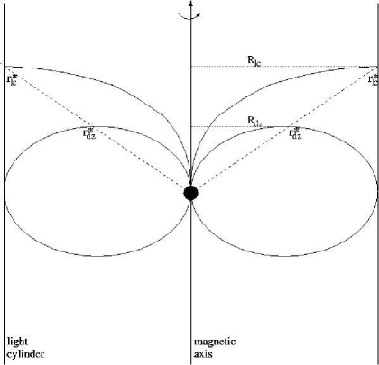
Figure 1: The geometry of the ‘mirror’ points in a plane projected onto the rotation axis. The null line intersects the dead zone and the light cylinder at $r_{dz}^{*}$ and $r_{lc}^{*}$ respectively.

In interpreting her results, Rankin (RII) notes that the inverse root dependence on period supports a dipole geometry: the radius of the polar cap, defined by the last field-line to close within the light-cylinder, scales with $P^{-0.5}$, and she therefore suggests that the two cones are both formed tangential to this same field-line at differing heights, with the emission of the inner cone lying below that of the outer cone. Following the logic of the dipole geometry, the outer cone at 1 GHz, whose angular radius is given in (1), is then formed at a period-independent height of 220km above the surface, and the inner cone at 110km.

This interpretation is difficult to reconcile with the frequency-to-radius mapping concept, whereby greater heights correspond to lower frequency emission, and theoretical efforts have been made to resolve this. Petrova (2000), Petrova $\&$ Lyubarskii (2000) and Qiao et al (2000) have suggested bimodal propagation models for the inner magnetosphere. However these models have been devised to explain the conal profiles, and it is as yet hard to see how they operate at the more fundamental subpulse level without implying that the inner and outer cones have identical subpulse behaviour (something which is rarely, if ever, observed).

In this paper we adopt an alternative interpretation: that the inner cone is also formed at the same height as the outer cone, but on a field-line closer to the magnetic axis. This suggestion is not new, and can be made consistent with the RS model by including surface multipole components of a specific form (Gil et al 1993, Gil $\&$ Sendyk 2000, Asseo $\&$ Khechinasvili 2002). But it would also enable the observational conclusions of Kijak $\&$ Gil (1997) and Kijak (2001) that emission heights decrease with decreasing period to be reinterpreted as emission cones moving closer to the magnetic axis.

Clearly identifying the true fieldlines on which emission occurs is a formidable observational task (Mitra $\&$ Rankin 2001, Kijak $\&$ Gil 2003). But in the present context, where we are pursuing the hypothesis of a purely dipolar field, any suggestion that different cones are located on different fieldlines is highly radical, since it would appear to imply that special field-lines are somehow chosen near the surface by the upward-moving particles - and the question arises how the particles can ‘know’ which field-lines to select! The dilemma can only be resolved by abandoning the concept, long-held by theoreticians, that the structure of the magnetosphere is determined, indeed driven, by conditions near the polar cap. The step we take here is to reverse this logic, and argue that events in the outer magnetosphere are the true ‘engine’ of the pulsar system, and that the observed polar region events are passive reflectors of these.

In their seminal work of 1969, Goldreich $\&$ Julian(GJ) divided the polar cap into a central region of outflowing (negative) particles and an outer annulus within which the current returned to the star. The outer boundary was defined, as in Rankin’s work, by the last closed field line. The inner boundary was defined by the field-line which intersects the light cylinder at the same point as the so-called null surface. The null surface is to first approximation the locus of the points on which the magnetic field is perpendicular to the rotation axis (see Mestel 1999, p536), and is physically significant since it is the surface separating regions of net positive charge from those of net negative charge on which the net charge density must be zero in a steady system. In an aligned pulsar the central region has negative charge density and the annulus positive. This polarity is reversed in the the counter-aligned model of RS, where the polar cap does not extend beyond the inner boundary.

The importance of the null surface was first realised by Holloway (1973), who pointed out that a charge-separated particle flow could never smoothly cross it, and that therefore an ‘outer gap’ of intense electric field would form, extending from the corotating dead zone to the light cylinder surface. In energetic young pulsars this gap is thought to be the site of gamma radiation (Cheng et al., 1986). In an axisymmetric system the null surface forms a cone of half-angle $\arctan{\sqrt{2}}\simeq{54.7^{o}}$, which intersects the light cylinder at an altitude of

$$r^{*}_{lc}={(\frac{3}{2})}^{\frac{1}{2}}R_{lc}={(\frac{3}{2})}^{\frac{1}{2}}\frac{cP}{2\pi}$$ (3)

and the dead zone at

$$r^{*}_{dz}=\frac{2}{3}R_{lc}=\frac{cP}{3\pi}$$ (4)

where $R_{lc}=\frac{cP}{2\pi}$ is the light-cylinder radius. The field-lines linked to these extrema enter the neutron star surface at angles which are in the period-independent ratio of

$${(\frac{r^{*}_{dz}}{r^{*}_{lc}})}^{\frac{1}{2}}=(\frac{2}{3})^{\frac{3}{4}}=0.74$$ (5)

(inner to outer). Through dipole scaling this ratio would then apply at any given height above the surface.

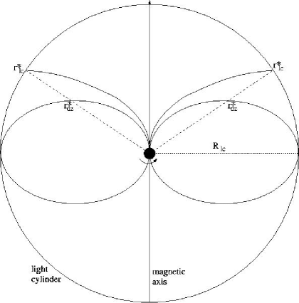
Figure 2: The geometry of the ‘mirror’ points of a near-perpendicular rotator in the plane of the observer‘s line of sight. The null line intersects the dead zone at $r_{dz}^{*}$ as before, and the light cylinder at a slightly reduced $r_{lc}^{*}$.

Of course real pulsars are inclined rotators and in their outer magnetospheres are far from axisymmetric and far from dipolar. Yet our line of sight passes over the magnetic pole with a low ‘impact’ angle in a plane where the magnetic field close to the surface is dipolar and hence axisymmetric about the pole to a first approximation. In this plane the null lines (along which the magnetic field is perpendicular the rotation axis) remain unchanged from those shown in Fig 1 for a precise dipole, and will make the same intersection with the dead zone at $r^{*}_{dz}$. However the light cylinder intersection will shift by an extent dependent on the angle of inclination. Fig 2 shows the most extreme case when the the magnetic and rotation axes are near-perpendicular, but still using a dipolar structure. The critical field-line for the inner cone has moved slightly outwards and the ratio of 0.74 has changed to 0.82.

In the more realistic Deutsch (1959) vacuum solution the field-lines near the light cylinder are swept back and would give an asymmetric and curved null lines at large inclinations. Furthermore the limiting field-lines defining the boundary of the dead zone will be perturbed, quite possibly in an asymmetric fashion. But we stress that for most pulsars these effects may only be of second order, and the ratio $(\frac{r^{*}_{dz}}{r^{*}_{lc}})^{\frac{1}{2}}$ may not stray far from the 0.74 to 0.82 range, especially since statistically the angles of inclination for pulsars cluster around $35^{o}$ and are only exceptionally found at high inclinations (see Figs 2 and 4 of RI, and Section 7 of this paper).

Taking the observed ratio of the inner to outer cone radii at 1GHz from (1) and (2) we obtain

$$\frac{\rho_{inner}}{\rho_{outer}}=0.75$$ (6)

The ratio is slightly higher at higher frequencies: 0.77 at 1.4GHz (Gil et al 1993), 0.78 at 4.75GHz (Kramer et al 1997). These ratios are consistent with the range indicated from the theoretical analysis above and suggest that we might identify the critical lines of GJ with the defining field-lines of the emission cones. This, in turn, points to an intimate relation between locations on the null surface - whose precise location may vary from pulsar to pulsar - and the pattern of emission above the polar cap. Somehow the outer magnetosphere and the polar regions mirror one another. This is an idea not present in polar gap models or space-charge-limited models for ‘slow‘ pulsars (eg RS, HAa,b, HM, HMZ), yet it immediately suggests an evolutionary link to the outergap models for fast pulsars (HSa,b). Thus we may suppose that, although now weak, outergap pair production may still play a crucial role in the radio emission process.

3 Conal type and the critical field-lines

The principal result of RII is that the profile types ($S_{t}$, M, T) show a dependence on period, yet no dependence on surface-related parameters such as $B_{s}$, the surface magnetic field strength, or the acceleration parameter $\frac{B_{s}}{P^{2}}$. In general, inner cones are found to form at shorter periods while outer cones form at longer periods, with an overlap range where both cones are present. If we assume that the outer cones and inner cones are formed by the same physical process at either null-line intersection, then this result can be reproduced by a simple geometrical argument. All that is needed is the assertion that a cone only forms when its corresponding intersection point lies within a fixed, period-independent, range of altitudes.

The simplest way to see this is to consider two pulsars, one of period $P_{1}$ and a faster one of period $P_{2}=(\frac{2}{3})^{\frac{3}{2}}P_{1}$. Then from (3) and (4) the outer cone of the slower pulsar is formed on exactly the same field-line as the inner cone of the faster. And since the opening angle of the null surface is independent of period, the magnetic field strength and the distance of the intersection from the surface remain the same, although now the intersection is with the light-cylinder of the faster pulsar rather than the dead zone of the slower pulsar. Thus whether a particular field-line appears as an inner or outer cone is determined solely by the pulsar period. This is completely independent of whatever physical criteria must be met in order to form a cone.

With this insight it is possible to use the observed period dependency of the various profile types to determine the range of periods within which emission cones are created. Rewriting (5), the distances, $r^{*}_{lc}$ and $r^{*}_{dz}$, of the intersection points from the star (which are proportional to $R_{lc}$, and hence to the period) are in the ratio

$$\frac{r^{*}_{lc}}{r^{*}_{dz}}=(\frac{3}{2})^{\frac{3}{2}}\simeq{1.84}$$ (7)

Let us then suppose that a cone only forms when the intersection points fall within $r^{*}_{min}$ and $r^{*}_{max}$. For $r_{dz}^{*}$ to be in this range, and hence for an outer cone to form, the pulsar’s period must, from (4), satisfy

$$3\pi\frac{r_{min}^{*}}{c}<P<3\pi\frac{r^{*}_{max}}{c}$$ (8)

Similarly, the period range for inner cone formation is, from (3),

$$2({\frac{2}{3}})^{\frac{1}{2}}\pi\frac{r{*}_{min}}{c}<P<2({\frac{2}{3}})^{\frac{1}{2}}\pi\frac{r{*}_{max}}{c}$$ (9)

The first range maps onto the second by the factor (7). As is shown in Fig 1, long-period pulsars with wide light-cylinders will be found to have only an outer cone because the light-cylinder intersection lies above $r^{*}_{max}$, and fast pulsars only an inner cone bcause the deadzone intersection is below $r^{*}_{min}$, with pulsars with an intermediate range of periods having two cones. This is exactly as reported in RII.

In RII Rankin finds that type $S_{t}$ and type T with only an inner cone have a mean period around 0.5s, type M with two cones have a mean period of 0.86s, and types T and D(double) with only an outer cone have a mean period of about 1.25s. If we assume that cones are only formed when the null-line intersection point lies between $r^{*}_{min}=20,000km$ and $r^{*}_{max}=70,000km$, then the range for inner cone formation is 0.32s to 1.15s, and consequently 0.6s to 2.15s for outer cones. This implies a double cone (M) range from 0.6s to 1.15s. These figures successfully reproduce the observed mean values, although the scatter around the mean is fuzzy (see tables in Rankin 1993b), and other hitherto unconsidered factors may be involved. Later in this paper it is suggested that the degree of electric screening near the magnetic pole may be such a factor, resulting, for example, in core-dominant type $S_{t}$ pulsars having a significantly lower range than the other categories.

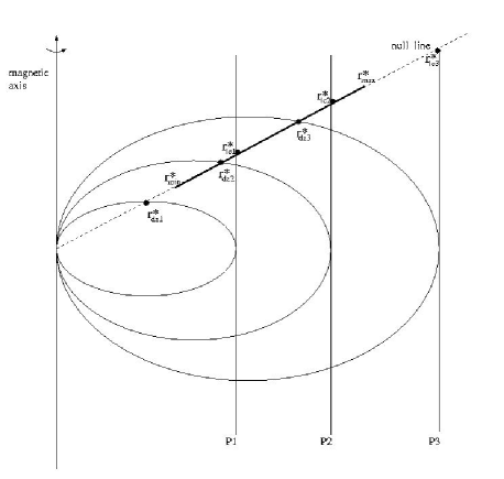
Figure 3: the vertical line (P1,P2,P3) show different possible positions for the light cylinder and their intersections with the null line ($r^{*}_{lc1},r^{*}_{lc2},r^{*}_{lc3}$). Each gives rise to a dead zone which intersects the null line at ($r^{*}_{dz1},r^{*}_{dz2},r^{*}_{dz3}$) respectively. Only $r^{*}_{dz2},r^{*}_{lc1},r^{*}_{dz3},r^{*}_{lc2}$ lie within the fixed range of heights indicated by $r^{*}_{min}$ and $r^{*}_{max}$ and therefore become mirror points

Note that it is the distance from the star which determines the appearance or non-appearance of a cone, and not, for example, the ambient magnetic field strength. This would depend on $B_{s}$, a factor which Rankin finds not to be statistically significant. Assuming a surface field of $B_{s}=10^{12}G$, the fixed range in radial distance translates into a poloidal magnetic field range of around $B_{min}=100G$ to $B_{max}=4000G$, a factor of $(3.5)^{3}\simeq{40}$. Actual estimates of $B_{s}$ vary by a factor comparable to this, and a criterion based only on field strength at the intersections could not reproduce the precision of the observed range without showing dependence on $B_{s}$. We are left with a criterion based on a tight range in intersection altitudes, or, equivalently, in star to null line communication times from 0.07s to 0.23s.

We stress that as yet no particular model for the creation of emission zones has been imposed. The whole purpose of this paper is to use the observations to define and constrain the emission model. What has been shown so far is that the observed dependence of profile morphology on period (and period alone) can be explained by a specifying a fixed and relatively narrow range of altitudes within which the ‘mirror’ site can fall. Thus the problem of morphology has been decoupled from the problem of devising an emission model. Observations seem to be forcing us to consider pulsar radio emission as a global pan-magnetosphere phenomenon, involving intercommunication between the polar cap and the outer gap. The required features of an emission model based on this interpretation are discussed in the next section.

4 The formation of emission nodes

In the previous sections it is argued that the observations of radio profiles support the existence of a feedback system betwen the star and the mirror points. This implies a flow of charged particles in both directions, guided by the magnetic fieldlines. Unless the electric fields parallel to the magnetic fields are universally screened (we discuss in Section 7 recent work by Harding and coworkers (HM,HMZ), who indeed find that in older pulsars this potential cannot be fully screened) it inevitably follows that the streams of charged particles will undergo an azimuthal drift, irrespective of how they are produced at either end. The sense of the drift will be the same for particles of either sign, and independent of whether they are moving outwards or inwards. It is also independent of whether we are dealing with a pulsar with rotation axis and magnetic moment in the same sense (as in the ‘inner accelerator’ models) or with an antipulsar (as in RS), where the axes are in opposing directions.

The picture we adopt is as follows: electrons are gradually accelerated outward on the critical mirror fieldlines from close to the surface to the the mirror points on the null line, where they initiate pair-production in the outergap. This production will not and cannot be prolific since the interacting photons will have low energy and will fail to initiate the massive pair cascades found in younger pulsars (Cheng et al 1986, HSa,b). Nevertheless sufficient low-energy positrons are then supposed to be available, either through pair-production or through interaction with another magnetospheric region (as envisaged in the previous section), or both, to cause a backflow of positive charge to the surface. The total current flow will be dominated by electrons, since in a steady state the net charge density must always be negative and close to the charge-separated GJ value. The drift will cause the positrons to return to the surface on a different fieldline from which the electrons came (see Fig 4), and they will be accelerated towards a different azimuthal location on the polar cap. Close to the surface the positron energies will be sufficient to trigger a pair-production ‘avalanche’ (as described in Michel 1992), which will cause electrons, either from the surface or trailing the avalanche (or both) to be accelerated upward into the magnetosphere. These will, in turn, continue to drift on their passage to the mirror regions. If theory can demonstrate that no particles from the surface are needed or even possible in this scenario, the entire model becomes sign-reversible and can apply to pulsars and antipulsars alike.

The central proposal here is that in a quasi-steady state the avalanches above the surface will be confined to discrete ‘emission’ nodes, arranged so that the flow forms a continuous yet finite stream of particles linking all the nodes (Fig 4). It is presumed that by remaining separated they avoid mutual interference and maintain conditions for pair-creation and the observed coherent radiation. In this section we describe and quantify the process by which these nodes are formed, and in the next section we consider how observations of subpulse drift can be interpreted as a movement of these nodes and be used as diagnostics of the conditions in a pulsar’s magnetosphere.

In the previous section it is argued that observations suggest that a high level of interconnectivity between the poles is a prerequisite for pulsar emission. Thus we may expect the particles created at the mirror points will feed both poles and ensure that particle drift at one pole is coordinated with that at the other. This supports a view that the mirror points are far from being the passive reflectors of events close to the surface, but rather drive the entire drifting phenomenon by means of null line interactions between the cones, and possibly through inter-pole links. Here we analyse an axisymmetric system at a single pole, although the ultimate intention is to apply the resulting estimates in the context of an inclined interactive magnetosphere.

The particle drift rate is estimated by an argument analogous to that of RS, but applied to an entire axisymmetric magnetosphere rather than confined to a polar cap. Inevitably the estimates will be less precise, but nonetheless useful. We consider first a configuration with an outer cone only (i.e. with no inner cone screening). If there is a potential drop of ${\Delta}V$ along the central magnetic axis from the surface to a height at the level of the dead zone intersection (see Fig 1), then the typical potential difference available over the cylindrical radius of $R_{dz}$ between the axis and critical fieldlines close to the deadzone is $-{\Delta}V$, since ¸there is a zero potential drop along field-lines bounding the dead zone and across the surface of the polar cap. Then taking the typical scale length of the electric field in the region of the dead zone as $R_{dz}$ we obtain $\frac{{\Delta}V}{R_{dz}}$ as a measure of the mean non-corotational electric field perpendicular to the magnetic field $B_{dz}$ at a cylindrical radius of $R_{dz}$. Using this we can estimate the mean magnetospheric drift rate relative to the corotating frame, and in the opposite sense to the star’s rotation, as

$$\mid{(\Omega_{D})^{{}^{\prime}}_{out}}\mid = \frac{1}{R}\frac{\mid{\bf\Delta{E}XB}\mid}{B^{2}}c$$ (10)

$$\approx {\frac{c{\Delta}V}{B_{dz}R_{dz}^{2}}}=\frac{2\pi}{P}\frac{{\Delta}V}{({\Delta}V_{max})_{out}}$$

where ${\bf\Delta{E}}$ is the variation in the electric field from the corotational value, and

$$({\Delta}V_{max})_{out}=\frac{2\Phi_{out}}{cP}\approx{\frac{{2\pi}B_{dz}R_{dz}^{2}}{cP}}$$ (11)

is the maximum potential available in the vacuum case, and $\Phi_{out}$ is the magnetic flux through the polar cap extending to its dead zone boundary (Sturrock 1971). Equation (10) gives zero net drift in the inertial frame when ${\Delta}V=({\Delta}V_{max})_{out}$, and corotation if ${\Delta}V=0$. Note that $(\Omega_{D})^{{}^{\prime}}_{out}$ is formally negative. The net particle drift rate in the inertial frame ($(\Omega_{D})_{out}=\frac{2\pi}{P}+(\Omega_{D})^{{}^{\prime}}_{out}$) is thus proportional to the level of screening within the magnetosphere, a quantity which may well be time-dependent. Henceforth, primed quantities will indicate that these are measured in the corotating frame.

An equivalent estimate can be made for the inner cone drift, although this will be more approximate since the field-lines will be swept back with a significant toroidal component, and particles are likely to have sufficient energy to leave the field-lines as they cross the light cylinder (Mestel et al, 1985). Assuming the potential difference of $\Delta{V}$ along the central axis now extends to a height at the level of the light cylinder/ null line intersection yields a potential difference $-{\Delta}V$ between the magnetic axis and the light cylinder at $R_{lc}$. This effectively assumes a zero potential drop along the null line between $r^{*}_{dz}$ and $r^{*}_{lc}$. In a more realistic model (i.e. that of Mestel et al 1985 or Shibata 1990) this potential drop is not zero and drives the closure of the current loop outside the light cylinder. Using now $R_{lc}$ as the scale length, this will produce the parallel formula to (10), namely

$$\mid{(\Omega_{D})^{{}^{\prime}}_{in}}\mid\approx{\frac{c{\Delta}V}{B_{lc}R_{lc}^{2}}}=\frac{2\pi}{P}\frac{{\Delta}V}{({\Delta}V_{max})_{in}}$$ (12)

with $({\Delta}V_{max})_{in}$ calculated from the magnetic flux $\Phi_{in}$ through the inner cone:

$$({\Delta}V_{max})_{in}=\frac{2\Phi_{in}}{cP}\approx{\frac{{\pi}B_{lc}R_{lc}^{2}}{cP}}$$ (13)

$\Phi_{in}$ is less than the full polar cap flux $\Phi_{out}$ by a factor of $\frac{r^{*}_{dz}}{r^{*}_{lc}}$, which from (5) gives

$$(\Omega_{D})^{{}^{\prime}}_{in}=\frac{r^{*}_{lc}}{r^{*}_{dz}}(\Omega_{D})_{out}=(\frac{3}{2})^{\frac{3}{2}}(\Omega_{D})^{{}^{\prime}}_{out}=1.84(\Omega_{D})^{{}^{\prime}}_{out}$$ (14)

Thus in the simplified magnetospheric model used here the particle drift rate in the inner cone is nearly twice as fast as that in the outer cone, if either is present alone.

Having established the parameters of the particle drift, we are now in a position to explore how many emission nodes are created. The inflow/outflow process in the outer cone will, in the corotating frame, circulate once around the cap in a time $\frac{2\pi}{(\Omega_{D})^{{}^{\prime}}}$. It is conjectured that the circulation sets up regular cycle, whereby the flow ‘visits’ $p^{\prime}$ nodes within $q^{\prime}$ turns and then repeats itself continuously (Fig 4). It follows that in each turn the flow makes $\frac{p^{\prime}}{q^{\prime}}$ descents to the cap, where

$$\frac{p^{\prime}}{q^{\prime}}\approx\frac{2\pi}{\mid{(\Omega_{D})^{{}^{\prime}}_{out}}\mid}\frac{c}{2r^{*}_{dz}} = \frac{3\pi}{2}\frac{2\pi}{P}\frac{1}{\mid{(\Omega_{D})^{{}^{\prime}}_{out}}\mid}$$ (15)

$$= \frac{3\pi}{2}\frac{(\Delta{V_{max}})_{out}}{\Delta{V}}$$

For the inner cone the equivalent calculation is

$$\frac{p^{\prime}}{q^{\prime}}\approx\frac{2\pi}{\mid{(\Omega_{D})^{{}^{\prime}}_{in}}\mid}\frac{c}{2r^{*}_{lc}} = (\frac{2}{3})^{\frac{1}{2}}\pi\frac{2\pi}{P}\frac{1}{\mid{(\Omega_{D})^{{}^{\prime}}_{in}}\mid}$$ (16)

$$= \frac{4\pi}{9}\frac{(\Delta{V_{max}})_{out}}{\Delta{V}}$$

The relations between n and $(\Omega_{D})^{{}^{\prime}}$ in the first lines of (15) and (16) are purely geometric relations, showing how $\frac{p^{\prime}}{q^{\prime}}$ depends on the drift rotation rate, the distance to the nodes from the mirror points and the period of the pulsar in the corotating frame. As will be seen in the next section, they enable us to set lower limits on $\frac{p^{\prime}}{q^{\prime}}$ in both cones, since in neither cone can $(\Omega_{D})^{{}^{\prime}}$ exceed the pulsar’s own rotation speed and counter-rotate (Ruderman, 1976).

The second lines of equations (15) and (16) express how $\frac{p^{\prime}}{q^{\prime}}$ measures the extent to which the optimum potential has been screened: the lower ${\Delta}V$ falls the larger $\frac{p^{\prime}}{q^{\prime}}$ will become. To compute $\frac{p^{\prime}}{q^{\prime}}$ we need estimates of $({\Delta}V_{max})_{out}$ and ${\Delta}V$. $({\Delta}V_{max})_{out}$ is obtained from (11):

$$({\Delta}V_{max})_{out}\approx{1.35}\times\frac{B_{12}}{P^{2}}10^{13}eV$$ (17)

where $B_{12}$ is the surface magnetic field in units of $10^{12}G$. For ${\Delta}V$ we can take a normalising value of, say, ${\Delta}V=5\times{10^{12}}$, which corresponds to the potential needed to accelerate electrons (positrons) to approximately $\gamma=9\times{10^{6}}$ at which radiated gamma-rays may trigger pair-creation. However it must be stressed that the intention of the model here is not to impose a value for $\Delta{V}$ or $\gamma$, but to find a way to measure them. Inserting (17) and the estimate for $\Delta{V}$ we obtain from (15) and (16)

$$\frac{p^{\prime}}{q^{\prime}}\approx{13}\frac{B_{12}}{P^{2}}(\frac{5\times 10^{12}}{{\Delta}V})$$ (18)

for the outer cone, and

$$\frac{p^{\prime}}{q^{\prime}}\approx{4}\frac{B_{12}}{P^{2}}(\frac{5\times 10^{12}}{{\Delta}V})$$ (19)

for the inner cone.

We can now return to our result of Section (3): that emission cones tend only to form when their mirror points lie between two fixed, period-independent altitudes. With the model here, the upper limit may be interpreted as a maximum distance of the mirror points above the emission nodes at which the required coherence of the emission nodes can be maintained close to the surface - a high degree of angular precision must be required to confine the node to its particular (possibly drifting) azimuth and prevent its ‘smearing’. At the other extreme, a too-dense clustering of nodes may cause interference between the electron and positron flows of adjacent nodes, preventing a steady flow between the surface and the mirror points.

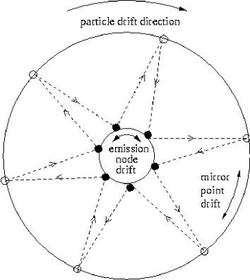
Figure 4: A view of the particle drift looking down onto the magnetic pole in the corotating frame. The motion of particles over distances of more than 20,000km to and from the ‘mirror’ points on the null line creates emission nodes immediately above the polar cap. The nodes, and their corresponding mirror points, may be stationary, or drift in either direction. The pattern shown corresponds to the simplest mode (i.e. all the nodes are created in a single turn).

5 Drifting subpulses

5.1 Introduction

The emission of many pulsars exhibits a systematic modulation known as drifting subpulses, whereby a succession of subpulses, identified here as the emission of adjacent nodes, appear in the pulse window and each gradually ‘drifts’ in the same sense across the window to the position of his neighbour within a timespan of $P_{3}$ rotation periods. The drift may be fast ($\approx$ 2 periods) or slow ($>10$ periods), and the pattern repeats itself, often for long stretches, before sometimes switching to a different ‘mode’ of emission.

In interpreting observations of drifting subpulses, the model suggested here shares with RS the picture of emission columns circulating around the magnetic pole. However the underlying flow which produces these columns, illustrated in Fig 4, is radically different and has greater flexibility. A steady system of stable emission nodes is created and maintained near the surface by a continuous, or quasi-continuous, flow of particles to and from the mirror points. Depending on the rate of particle drift, which in the corotating frame can have only one sense, the nodes may be stationary, or precess positively or negatively around the magnetic pole. An equal number of pair-producing regions on the outer gap, either at the dead zone boundary ($r^{*}_{dz}$) or at the light cylinder ($r^{*}_{lc}$), will precess in tandem (Fig 4). In theory a very wide range of emission systems can be generated in this manner, some highly complex and chaotic. However the ‘mode’ selected by the pulsar will reflect the value of $\frac{\Delta{V}}{\Delta{V_{max}}}$.

There is a fascinating everyday analogy to the process suggested here. If a camcorder linked to a television set is pointed at the screen in a completely darkened room, and if an initial instantaneous flash (such as the striking of a match) occurs between the screen and the camcorder, then the image of the flash appears on the screen and feeds back into the camcorder. The image on the screen will then constantly change, creating patterns which may be regular or chaotic, depending on the angle at which the camcorder is held about its axis. It is a classical demonstration of how complexity can arise even in a simple feedback system: complexity of outcome does not imply complex input.

In the previous section we estimated the particle drift-rate in the corotating frame. This is the appropriate frame for the calculation of the driving electric field, but the observed number and drift of the nodes depend critically on the observer’s frame of reference. For example, if the observer were rotating at a rate less than, but in the same sense as, the corotating drift-rate of the particles, their apparent drift relative to the observer would be smaller than in the corotation frame, and he would see a larger number of nodes for every rotation in his frame. These nodes would remain in the same sequence as in the corotating frame, but would begin to repeat before a single turn was completed. If the observer moved counter to the drift, he would see fewer nodes in a single turn, but on the second and later turns the nodes would appear to overlap, and the order of the nodes round the axis would therefore be changed. This is an important point, since the pulsar observer in his inertial frame will always turn counter to the sense of the particle drift in the corotating frame, and may well observe a node pattern very different from that in the corotating frame (as will be seen in the case of PSR0943+10, discussed in the next section).

5.2 Critical parameters

We consider a distant observer’s view of the drift, and relate the underlying particle drift in his inertial frame to the number of nodes and to the observable quantity $P_{3}$. We begin by adapting the estimates in (15) and (16) to the inertial frame drift $(\Omega_{D})_{out/in}=\frac{2\pi}{P}+(\Omega_{D})^{{}^{\prime}}_{out/in}$, but still assuming that the pulsar is aligned. In this frame the observer sees p nodes created in q turns by successive inflows and outflows (where p and q are integers with no common factors) so that every q th node is sequentially linked as the particle flow circles the pole. Then

$$\frac{p}{q}\approx\frac{2\pi}{\mid{(\Omega_{D})_{out}}\mid}\frac{c}{2{r}^{*}_{dz}}$$ (20)

for the outer cone, and

$$\frac{p}{q}\approx\frac{2\pi}{\mid{(\Omega_{D})_{in}}\mid}\frac{c}{2{r}^{*}_{lc}}$$ (21)

for the inner cone. Note that $\frac{p}{q}$ and $\frac{p^{\prime}}{q^{\prime}}$ in the notation of the previous section are equivalent parameters in the inertial and corotating frames respectively.

Each of the particle path distances ${r}^{*}_{dz}$ and ${r}^{*}_{lc}$ defines a mean transit time ($\tau_{dz}$ or $\tau_{lc}$ in units of P, the pulsar rotation period) from the nodes to the mirror points and back in the outer and inner cone respectively, so that

$$\tau_{dz}=\frac{2{r}^{*}_{dz}}{Pc}\approx\frac{2}{3\pi}=0.212$$ (22)

for the outer cone, and for the inner cone

$$\tau_{lc}=\frac{2{r}^{*}_{lc}}{Pc}\approx(\frac{3}{2})^{\frac{1}{2}}\frac{1}{\pi}=0.395$$ (23)

where the estimates are those for the aligned rotator as in (3) and (4). The inner cone value is almost double that of the outer cone, reflecting the greater distance the flow has to travel to the light cylinder intersection.

In practice, q will be taken as low ($<10$) and any more complex flow will be seen as a modulation of a basic (p,q) pattern. Since the particle drift in the inertial frame cannot exceed the rotation speed (Ruderman 1976), we demand that $\mid{(\Omega_{D})_{out/in}}\mid<\frac{2\pi}{P}$. Hence from(20) and (21)

$$\frac{p}{q}>\frac{1}{\tau_{dz}}\approx\frac{3\pi}{2}=4.7$$ (24)

for the outer cone, and

$$\frac{p}{q}>\frac{1}{\tau_{lc}}\approx(\frac{2}{3})^{\frac{1}{2}}\pi=2.6$$ (25)

for the inner cone.

5.3 Conditions for steady subpulse drift

To turn the approximate results (20) and (21) into exact equations we need to incorporate into $(\Omega_{D})_{out/in}$ a term which takes account of the rate at which the nodes move around the magnetic axis. After a total time of $\hat{P}_{3}=p{P_{3}}P$ (following the notation of RS for $\hat{P}_{3}$) the entire ring of emission nodes will have presented itself to the observer. Thus in a smoothly-flowing system (20) can be rewritten as

$$(\Omega_{D})_{out}=\frac{2\pi}{\tau_{dz}}\frac{q}{p}+\frac{2\pi}{{\hat{P}}_{3}}=\frac{2\pi}{P}\times\frac{q}{p}[\frac{1}{\tau_{dz}}+\frac{1}{q{P_{3}}}]$$ (26)

In the equivalent expression for $(\Omega_{D})_{in}$, $\tau_{lc}$ replaces $\tau_{dz}$. As long as $\mid{P_{3}}\mid>1$, the first term in the brackets of (26) always dominates over the second. Hence the drift will be only a fraction of the true particle drift. In general, there is no preference for the sign of $P_{3}$, and the observed drift may appear to be in the sense of rotation or the reverse. When both inner and outer cones are present, their nodes may conceivably have differing drift directions. Opposing drifts at differing longitudes of the pulse window have been observed in PSR0540+23 (Nowakowski, 1991).

The picture implied by (26) is of a simple integrated system with a near-continuous even flow of particles streaming from each node up to the mirror points and back, successively visiting all of the drifting nodes in the system cycle time (evaluated in (28) below) before returning to meet the node from which it set out. More realistically, the flow may be made up of ‘packets’, possibly separated by the node-mirror point travel time ($\approx{0.1P}secs$), but sufficiently continuous for us to ‘see’ each node at our sampling rate of P seconds. Should this occur the observed emission could be separately modulated by phase and by intensity.

In practice, observers will be able to measure $P_{3}$ (though not necessarily its intrinsic sign), possibly also p (as in PSR0943+10), and will wish to infer q and $\tau_{dz/lc}$. From the analysis so far they will have at hand conditions (24/25), and equation (26). But there is one further useful constraint which links the known and unknown quantities. This essentially geometric point arises because the magnitude of the residual angle drift, represented by the last term in (26), must be small enough (i.e. $\mid{P_{3}}\mid$ large enough) to ensure that the system has just p nodes and does not accelerate/decelerate to a (p-1) or (p+1) system (depending on the sign of $P_{3}$). In other words, for a given p, q and $\tau_{dz/lc}$ there is a critical $\mid{P_{3}}\mid$ below which a steady system cannot form.

In establishing this condition we will examine in greater detail, in equations (27) to (34), the geometric and physical features of a near-steady conal system which underlie the result (32). The following equations apply to either cone, but are illustrated using outer cone parameters.

Consider particles being emitted simultaneously from all p nodes. The flow from each node will then call at its next successive (not necessarily adjacent) node after just $\tau_{dz}\approx{0.212}$ periods, the fundamental unit of time for the outer cone subpulse system of the pulsar, which will in general depend on both P and $\alpha$ in an non-aligned system. In this time the node will appear to advance by

$$\frac{2\pi}{\hat{P}_{3}}\tau_{dz}\approx\frac{4}{3pP_{3}}radians=\frac{76.4^{o}}{pP_{3}}$$ (27)

The node will drift smoothly if this angle is small compared with the angular extension of the node. The flow will then continue to the next node, and by the time the round trip is complete, all p nodes will have been visited in the system cycle time

$$t_{c}=p\tau_{dz}\approx{0.212pP}secs$$ (28)

and the flow will have traversed a total angular distance of

$$2\pi{q}+\frac{2\pi}{\hat{P}_{3}}t_{c}=2\pi{q}+\frac{2\pi}{P_{3}}\tau_{dz}\approx{2\pi{q}+\frac{4}{3P_{3}}}$$ (29)

This result can be equivalently obtained from (26) by multiplying $(\Omega_{D})_{out}$ by $t_{c}$.

The residual final term in (29) (which we will refer to as the cycle drift angle) is given by

$$\Theta_{c}=\frac{2\pi}{P_{3}}\tau_{dz}\approx{\frac{4}{3P_{3}}}=\frac{76.4^{o}}{P_{3}}$$ (30)

and represents the net angle through which the system has drifted in a single cycle. It is a useful observable parameter in determining the characteristics of the system, and it enables us to determine how many cycles, $N_{c}$, are required to rotate the entire system through a full circle, namely

$$N_{c}=\frac{2\pi}{\Theta_{c}}=\frac{P_{3}}{\tau_{dz}}\approx\frac{3\pi{P_{3}}}{2}=\frac{P_{3}}{0.212}$$ (31)

$N_{c}$ must be an integer if the system is to be closed and have a simple repeatability. Then any ‘streaky’ features in the underlying flow will share the $\hat{P}_{3}$ periodicity, the phase periodicity of the nodes, since

$$\hat{P}_{3}=N_{c}{t_{c}}$$ (32)

For the inner cone the net drift angle, $\Theta_{c}$, is significantly larger ($\frac{141^{o}}{P_{3}}$) and $N_{c}\approx\frac{P_{3}}{0.395}$.

A further significance of the cycle drift angle is that it can determine, for a given $P_{3}$, how close the p-node system is to going over into an $p+1$ or $p-1$ system. As $P_{3}$ reduces, the cycle drift angle grows (see (30)), and if the system is to keep its identity as a rotating p-node pattern, $\Theta_{c}$ must not exceed the separation ($\frac{2\pi{q}}{p\pm{1}}$) between successive nodes in the $p+1$ or $p-1$ system (depending on the sign of $P_{3}$). Using (31), a minimum $P_{3}$ for a given p is therefore set by

$$\mid{P_{3}}\mid>\tau_{dz}\frac{(p\pm{1})}{q}\approx\frac{2(p\pm{1})}{3\pi{q}}=0.212\frac{(p\pm{1})}{q}$$ (33)

where the positive sign applies if $P_{3}$ is negative, or more simply,

$$N_{c}>\frac{p\pm{1}}{q}$$ (34)

Combined with the conditions (24)/(25), (33) and its inner cone equivalent enable useful limits on p and q to be set. It is immediately clear that for simple systems with q=1, a high value for p will require a high $P_{3}$ (i.e. a low drift-rate): for example, if p=20 in an outer cone geometry, $P_{3}$ must exceed 4. This point is particularly relevant to PSR0943+10, discussed in the next section.

Using his estimate for (p,q) and taking a plausible value for $\tau_{dz}$, the observer could now evaluate the drift-rate of the particles, and hence infer the potential difference $\Delta{V}$ from (18). But in pulsars which exhibit great regularity in their subpulse drift it is possible to take one further step. Note that a particularly simple class of drift states can exist if the pulsar adopts a $P_{3}$ such that the value of the square bracket in (26) is an integer or a simple fraction. This would result in a harmonic relation between the underlying particle drift and the star‘s rotation rate, a factor which would make the flow steady, sustainable and hence conducive to the formation of emission nodes. It may even be a precondition for a pulsar to be observable. In an outer cone, $\frac{1}{\tau_{dz}}$ is 4.7 in the aligned dipole case (from (22)), and the mean value of this term will not differ greatly at inclinations with low $\alpha$. This suggests that in regularly drifting pulsars the value of the square brackets is 5, and that the harmonic relation to the rotation rate would be especially clear if p were a multiple of 5. Furthermore $P_{3}$ has to be positive in nearly-aligned pulsars. From (26) and (31) the harmonic condition implies values for $P_{3}$ and $\tau_{dz}$ of

$$P_{3} = \frac{1}{5}(N_{c}+\frac{1}{q})$$ (35)

$$\tau_{dz} = \frac{1}{5}(1+\frac{1}{qN_{c}})$$ (36)

Pulsars which exhibit highly regular drifting subpulses may be expected to have parameters which satisfy these equations.

5.4 Mode-changing

Many well-known pulsars maintain a steady or near-steady drift behaviour over many periods (even over thousands of periods in the case of PSR0943+10 discussed in the next section). These pulsars appear to have low values of the inclination angle $\alpha$ (RI), and hence the axisymmetric model of the previous section would seem a reasonable approximation of their conditions. Examples are PSR0031-09 (Vivekanand $\&$ Joshi 1997, Wright $\&$ Fowler 1981b), PSR1944+17 (Deich et al. 1986), PSR2319+60 (Wright $\&$ Fowler 1981a), PSR 1918+19 (Hankins $\&$ Wolszczan 1987), and, most recently, PSR0809+74 (Lyne $\&$ Ashworth 1983, van Leeuwen et al 2002).

However each of these pulsars also has at least one alternative - and equally stable - drift mode, so a number of steady solutions to equation (26) must exist in a single pulsar. By inserting integral values of $N_{c}$ and q into (35) and (36) an infinite series of discrete possible stable harmonic states can be generated. Which of these is selected by a particular pulsar - at a particular time - may be determined by allowed values of $\Omega_{D}$ and $\tau_{dz}$. These are likely, in turn, to depend on the current flow generated from the emission nodes close to the polar cap and on the precise height of the null line above them (which are interrelated parameters according to the recent outergap model of HSa,b). In the outer cone, particularly simple harmonic ratios (26) between $\Omega_{D}$ and the rotation of the star (such as $\frac{1}{2}$,$\frac{1}{3}$,$\frac{2}{3}$,$\frac{1}{4}$, $\frac{3}{4}$, etc) may only be attainable if if p is a low multiple of 5 and not a multiple of q. A mode change to another harmonic state can occur providing $N_{c}$, p and q satisfy the constraints (24) and (34). A change in $N_{c}$ will cause a change in $P_{3}$, a change in p will cause a change in $P_{2}$, the observed frequency-dependent subpulse separation, and a change in $\frac{q}{p}$ will change the harmonic ratio (26).

Mode changes may (from (36)) also be accompanied by changes in $\tau_{dz}$, the particle travel time between the nodes and the mirror points and back, therefore requiring a shift in the emission region. Studies of the mode changes in PSR0031-07 by Vivekanand $\&$ Joshi (1997) and Wright $\&$ Fowler (1981b) suggest a progressive shrinking of the profile from mode to mode, which may support this interpretation. More recent work by van Leeuwen et al (2003) argues for a similar effect in PSR0809+74. However in all the pulsars identified above the drift repetition rate, $P_{3}$, although stable for a while, shortens abruptly and successively through two or three discrete values before returning to the highest $P_{3}$ in a quasi-cyclical manner. A possible model which emerges for this class of pulsars is one of progressively decreasing levels of screening and build-up of potential, followed by a sudden return to high screening, and a cycle is established.

The quasi-stability of the general chaotic systems suggests that, once achieved, the pulsar’s potential will remain in such a state, subject only to a gradual secular change, then return to either the original state or some ‘closer’ alternative mode. Key to the stability of the subpulse behaviour during these transitions is the speed with which the nodes reconfigure themselves following a change: if the relaxation timescale is too long, the pulsar emission may never settle down to a steady pattern. The intermittent, but non-periodic, activity observed in the the core regions of many pulsars (Seiradakis et al. 2000), whatever its origin, is evidence that most magnetospheres are indeed in a quasi-chaotic state.

6 A Model for PSR0943+10

6.1 Background

PSR0943+10, with a period of 1.1sec and $B_{12}=2$ (see DR), has very typical pulsar parameters, but exhibits an extraordinarily precise alternating drifting pattern (in the dominant B mode) and occasionally switches to an apparently disordered Q mode (Suleymanova $\&$ Izvekova, 1984). It is of great interest here partly because the inferred angle of inclination between the magnetic and rotating axes is just $11^{o}-15^{o}$, suggesting comparison with the aligned model used to estimate paramters in the previous section. But it is also of interest since Deshpande and Rankin (2000)(DR), in their recent detailed study of this pulsar, have provided the only example so far where N, the total number of the emission nodes, has been directly deduced from a precise measurement of the circulation rate. The exceptionally stable subpulse pattern with $P_{3obs}=1.867$ is shown to have exactly N=20 drifting nodes, with the observed drift in the same sense as the presumed ${\bf E\times{B}}$ particle drift.

An interpretation in terms of the present model is somewhat hampered by the fact that the line of sight trajectory of this pulsar is too oblique for observers to determine conclusively whether we are seeing the geometry of an inner or an outer cone (DR give two alternative good fits with $\alpha=11.6^{o}$ for an inner cone, and $\alpha=15.4^{o}$ for an outer cone). However the facts that $P_{3}$ is positive and that the pulsar is almost aligned suggest (from the discussion in Section 5) that the emission is from an outer cone. Since N is known (and assuming initially that we are seeing a single system, so that N=p), we can immediately estimate the particle drift-rate from (20) and (22) as

$$(\Omega_{D})_{out}\approx\frac{2\pi}{P}\frac{q}{4}$$ (37)

It can be immediately seen (and is formally expressed in (24)) that $q<{4}$ if $(\Omega_{D})_{out}$ is to be less than the pulsar rotation rate.

6.2 The B mode

The relatively small value of the observed $P_{3}$ enables us to further constrain the possible configurations. Firstly, for either type of cone we can see that for p=20, q=1 neither the outer cone condition (33) nor its inner cone equivalent is met, so, in the observer’s frame, all 20 nodes cannot be linked in a single traverse round the polar cap. Systems with an even value of q can also be excluded since they would require an odd number of nodes. Thus q=3 remains the only possibility if all nodes belong to the same system. However it is theoretically possible that we are observing 2 independent but interlocking systems of 10 nodes each, or 4 of 5 nodes etc. These systems cannot satisfy the criterion for q=1, but are possibilities with q=3. Nonetheless, the system’s observed clockwork regularity argues powerfully for a single integrated system, and therefore the most likely candidate is one with p=20, q=3.

Accepting this as our working hypothesis, what characteristics will the system possess? It will connect every third node at time interval (from (22)) of approximately 0.212P until all 20 nodes are visited, taking $t_{c}\approx{20}\times 0.212=4.24$ periods for the cycle. Assuming only that $P_{3}$ is in the region of 1.85, then from (30) the net angular drift of the system after the time $t_{c}$ will be approximately

$$\Theta_{c}\approx\frac{76.4^{o}}{1.85}=41.3^{o}$$ (38)

implying a net drift of about $2^{o}$ per node visit. The nodes are $18^{o}$ apart, so node visits are separated by $3\times{18}+2=56^{o}$.

To make the model precise we need more exact values for both $P_{3}$ and $\tau_{dz}$. Noting that the net drift angle $\Theta_{c}$ is close to $40^{o}$, gives from (31) an estimate of $N_{c}$ as 8.73, close to the integer 9. Let us therefore suppose that in reality $N_{c}$ is exactly nine, giving the flow an exact repeatability. Then the further conditions (35/36), which would apply if the flow is harmonically coupled to the star’s rotation predicts $P_{3}$ and $\tau_{dz}$ to be

$$P_{3} = \frac{1}{5}(9+\frac{1}{3})=1.86666....$$ (39)

$$\tau_{dz} = \frac{1}{5}(1+\frac{1}{3\times 9})=0.2074$$ (40)

(39) is precisely the observed value of $P_{3}$ and is the only value between 1.66 and 2.00 which can give harmonic coupling (these values corresponding to $N_{c}$ at 8 or 10).

From the the value of $\tau_{dz}$ in (40) we obtain an adjusted cycle time of $t_{c}=20\times{0.2074}P=4.15P$, exactly one ninth of the observed $\hat{P}_{3}=37.35$. With the deduced values for $P_{3}$ and $\tau_{dz}$ it follows that the particle drift in the observer’s (inertial) frame has an angular speed of

$$(\Omega_{D})_{out} = \frac{2\pi}{P}\times\frac{3}{20}[\frac{1}{0.2074}+\frac{1}{3\times{1.867}}]$$ (41)

$$= \frac{2\pi}{P}\times{0.7500}$$

so the particle drift is exactly three quarters of the star’s rotation rate. This suggests that the pulsar has adjusted both the path length of its flow and its potential field so that this coupling occurs.

Thus we are left with a model of extraordinary harmony: $P_{3}$ is 9 times the basic timescale of 0.2074P, the particle drift circulates round the magnetic axis 3 times in exactly 4 periods, requiring $20\times{0.2074}P$ ($=4.15P$) to complete the 20-node cycle, which then repeats itself exactly 9 times before returning to its starting point.

In the corotating frame the picture is even simpler. The angular speed of the the particles $(\Omega_{D})^{{}^{\prime}}_{out}$ will now be exactly one quarter of the pulsar rotation rate, and in the opposite sense. The equivalent equation to (41), relating the particle drift to the $p^{\prime}$ and $q^{\prime}$ seen in the corotating frame will be

$$(\Omega_{D})_{out} = -\frac{2\pi}{P}\times\frac{1}{20}[\frac{1}{0.2074}+\frac{1}{1\times(3\times 1.867)}]$$ (42)

$$= -\frac{2\pi}{P}\times{0.2500}$$

It is clear that p remains unchanged from p at 20 but now $q^{\prime}=1$, whereas q=3. Thus in this frame all the nodes are visited consecutively in a single turn, with the cycle still taking 4.15 periods, but an observer would see a much slower node drift $P_{3}=3\times{1.867}=5.600$. This finally enables us to estimate the underlying potential difference required to support this drift. From (10) it follows that three quarters of the available electric potential is screened, thus leaving a potential (from (18) with $B_{12}=2$, P=1.1, $\frac{p^{\prime}}{q^{\prime}}=p^{\prime}=20$) of $\Delta{V}=5.3\times 10^{12}eV$, enough to accelerate particles to $\gamma\approx 10^{7}$.

6.3 The Q mode

For the irregular Q-mode, which comes on abruptly and shatters the clockwork regularity of the B-mode, an interpretation is more difficult. But a number of features stand out. DR note that at the outset there is a roughly 4P intensity fluctuation present, which could be the residual of the underlying particle drift periodicity of the 20 node system. This periodicity is never observed in the smoothly-flowing B-mode, whose variations are those of phase rather than intensity. We would interpret this as the particle flow between the surface and the nodes becoming disordered, though possibly even continuing to drift at a rate similar to that in the B-mode. The particles now flow in ‘packets’ rather than streams, and give rise to the ‘streaky’ emission which DR report.

But why does the flow become disordered? The most prominent feature in the Q-mode power spectrum, spread across most of the pulse window, equivalent to a periodicity of $P_{3}=1.293$, arises from occasional periodic bursts against a generally chaotic background. But with p=20 this drift no longer satisfies the condition (33) for any integral value of q. The possible suggestion is that the Q-mode has become disordered because $P_{3}$ has suddenly changed to a value which destabilises the 20-node pattern. Substituting the new $P_{3}$ into (30) and (31) yield a net drift angle, $\Theta_{c}$, of $59.1^{o}$ and $N_{c}$=6.1, yet again giving almost round figures.

Assuming therefore that the flow is attempting to achieve a regular stable system with $N_{c}=6$ precisely, and taking q=2, we obtain from (36/35) $\tau_{dz}=0.210$ and $P_{3}=1.300$, close to the observed but intermittent $P_{3}$, but requiring a slightly larger $\tau_{dz}$. Thus we may interpret the Q-mode as a failed attempt by the pulsar to switch to a second harmonic state with (from (26)) a particle drift of exactly half the pulsar rotation rate. It fails because such a drift is not consistent with 20 nodes, and requires them to be reduced. So why doesn’t the pulsar simply reduce the number of nodes to a compatible figure? Possibly because the current flow from and to the polar cap, presumably proportional to the number of nodes, has to be maintained at some fixed rate whatever the level of the electric potential.

Note that in the catalogue of ‘drifting’ pulsars of Rankin(1986) there are no fewer than 6 examples of pulsars with a $P_{3}$ of 2.1-2.2 (the alias of $P_{3}$=1.85), out of a total of 28. This seems a very high proportion, and it is possible that some - even all - these pulsars have exactly the same $P_{3}$. In addition to PSR0943+10, the catalogued pulsars are PSR2303+30, PSR0834+06, PSR2021+50, PSR2310+42 and PSR2020+28. PSR1933+16 has also been reported to show this phenomenon (Oster et al., 1977, Wolszscan, 1980)) and PSR1632+24 is a clear example (Hankins $\&$ Wolszczan, 1987). It seems there is evidence of a pulsar subpopulation with this on-off property (see Fig 4 of Rankin 1986). Clearly aliasing bedevils a proper analysis of the drifting behaviour of many pulsars, and more careful investigation is needed and could provide a useful test of this model.

7 The inclined rotator

Many of the relatively stable (and slow-drifting) pulsars appear to have low anges of inclination (see the examples listed in Section 5.4 and the tables of Rankin 1993b). This is unlikely to be a coincidence. Near-axisymmetric geometry means that quantities such as $r^{*}_{dz}$, the distance between the outer nodes and inner nodes, and its associated time scale, $\tau^{*}_{dz}$, remain roughly constant along the trajectory of the nodes. Thus conditions for pair-creation will not vary too much as the nodes drift. Fig 5 shows graphically how that, although the observed nodes circulate the magnetic axis, the mirror nodes enclose both the magnetic and the rotation axis. The slow drift in pulsars of this type, often observed to be many orders of magnitude slower than the rotation period, therefore implies that the locations of the mirror nodes are almost precisely corotating with the dead zone surface on which they sit, although the real particle flows which produce them will be far from corotating.

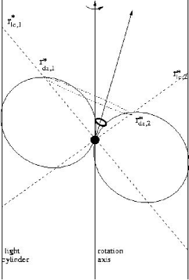
Figure 5: The emission geometry for pulsars at a low angle of inclination. Note that although the rings of nodes both near the pusar surface (dark ring) and their mirrors on the null surface (finely dotted ring) encircle the magnetic axis, only the mirror ring at also includes the rotation axis. A low node drift (ie low subpulse drift-rate) therefore implies near corotation of the outer nodes on the surface of the corotating dead zone.

In near-axisymmetric conditions it is easy to see how drifting subpulses and the resulting emission cones can be maintained. But the model here, in contrast to the RS model, requires interaction between widely-separated regions of the magnetosphere, and it cannot be assumed that conditions for the creation of emission cones can persist for larger values of $\alpha$.

Figs 6, 7 and 8 show the fiducial plane which contains both the rotation and magnetic axes for increasing angles of inclination. For simplicity, at all angles a pure dipole geometry is assumed rather than the more exact, but more complex, Deutsch (1956) solution for a rotating dipole in vacuo (Arendt $\&$ Eilek, 2001). Indeed an even better approximation may be the complex fully-corotating field derived analytically for inclined geometries by Beskin et al (1993). Nonetheless our assumption has the virtue that the null surface still intersects the plane in two straight lines (as in the aligned case), but now makes differing angles with the dipole axis. Here we focus attention on the changing locations of the mirror points in this plane as $\alpha$ increases, and their possible interactions with other features in the azimuthal plane (the plane perpendicular to the rotation axis).

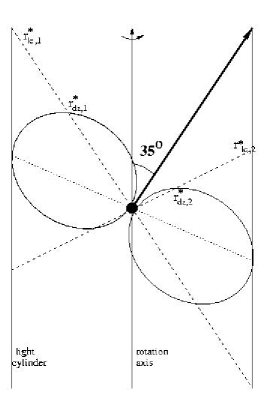
Figure 6: Connectivity at $\alpha=35.3^{o}$. At this inclination the ‘jet’ meets the light cylinder at the same colatitude as the light cylinder mirror point, enabling interaction between these regions. Furthermore the dead zone osculating point is capable of interaction with the opposite light cylinder mirror point.

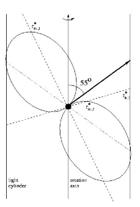
Figure 7: Connectivity at $\alpha=54.7^{o}$. At this inclination the ‘jet’ colatitude coincides with that of the osculating point of the dead zone. For $\alpha$ larger than this the possibilities of regional interaction become greatly reduced

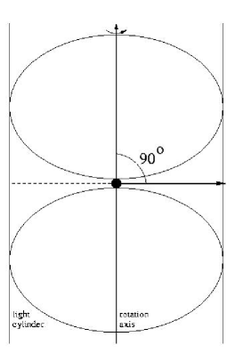
Figure 8: Connectivity at $\alpha\simeq{90^{o}}$. At near-perpendicular geometries interaction is possible between opposite poles through the opposing deadzone osculating regions, and even through jet-to-jet contact

One such feature is a polar ‘jet’: It is known that most pulsars display activity in the core region of their profile, so we can reasonably assume that a stream of particles emanates from or infalls onto the magnetic pole along field-lines in a close bundle around the polar field-line. If the pulsar is not aligned with its rotational axis, this stream will cross or ‘impact’ the light-cylinder at an angle which for simplicity we will assume to be $\alpha$. However, near the light-cylinder the spinning of the star will twist the polar field-lines backwards in azimuth, together with the streaming particles, forming a ring-like structure at this colatitude.

A second possibility is the osculating boundary of the dead zone at the light cylinder, represented in Figs 6 and 7 by the extremes of the dotted lines. As is pointed out in Mestel (1999), particles constrained to rigidly corotate close to the light-cylinder can be expected to achieve sufficient inertia to drift across field-lines. These particles would rotate more slowly than the rigid rotation and form a ring around the rotation axis at the appropriate colatitude, encountering open fieldlines and possibly contributing to screening.

As $\alpha$ increases from zero, the angle between the rotation axis and $r^{*}_{lc,1}$, decreases monotonically, until a point is reached where this angle is itself equal to $\alpha$. This is at

$$\alpha=\arctan{(\frac{1}{\sqrt{2}})}=35.3^{o}$$ (43)

At this angle the ‘impact point’ of the core jet is in the same azimuthal plane as one of the mirror points of the inner cone (see Fig 6). In the same configuration it can be seen that other mirror point of the inner cone (at $r^{*}_{lc,1}$) is at almost the same angle ($=2\alpha=70.6^{o}$) to the rotation axis as the osculating point of the dead zone($=66.8^{o}$) and provides a second opportunity for azimuthal interference, this time between the second mirror point in this plane and, via the osculating point, the inner conal structure of both poles.

At an inclination angle of

$$\alpha=\arctan{\sqrt{2}}=54.7^{o}$$ (44)

a further geometric coincidence occurs (Fig 7) where the magnetic axis and the dead zone contact are at the same colatitude on opposite sides of the rotation axis. This suggests a direct interactive link between the polar jet and the outer cone near the light-cylinder in the azimuthal ring perpendicular to the rotation axis. The locus of the inner cone mirror points at the light cylinder must also cross this ring at two places, so both cones and the core are capable of interacting in a single system. This may account for the complex behaviour of PSR 1237+25 (Hankins $\&$ Wright 1980), a pulsar which is thought to have an inclination angle of $53^{o}$ (Rankin 1993b), and in which the behaviour of the inner and outer cone are clearly coordinated.

The above picture of interactivity, based only on a geometric analysis of the relative locations of the null surface intersections and the magnetic axis, lends a surprising degree of support to the results of RI, in which Rankin assembles two histograms of the numbers of each profile type versus $\alpha$ in 10-degree bins. As pointed out in Section 2, these results require extraneous - but not unreasonable - assumptions concerning the apparent angular size of the core region, yet they display a dependency on $\alpha$ which strongly supports the interactive picture developed here. The first (Fig 2 of RI) shows the histogram for pulsars with a prominent core component (type $S_{t}$), a young population with a mean age around $10^{6}$ yrs. This reveals a sharp peak at $35^{o}$, which tails off up to $65^{o}$. In a further comment (in RII) on the distribution of type $S_{t}$ pulsars, Rankin finds that $S_{t}$ pulsars can be divided into two sub-populations, one having no cones at any frequency and the other developing inner cones at higher frequencies. The only factor discriminating between these populations is that the former cluster around $35^{o}$ and the latter around $50^{o}$.

Using our interactive model we can interpret these observations to mean that in young pulsars with narrow light-cylinders the core component only appears when it is possible for the core jet to azimuthally interact, via a non-equatorial ring structure, with the mirror regions of the inner cone, and that that it is further enhanced by the inner cone’s link to the dead zone (and hence to the outer cone). $\alpha=35^{o}$ therefore represents a ‘resonant’ inclination which encourages a strong jet, yet inhibits the formation of cones. For larger $\alpha$, azimuthal interaction between the jet and the mirror regions remains possible in planes other than the fiducial plane, but will lack the $180^{o}$ symmetry as the pulsar spins. As we approach the inclination where the jet and the dead zone can interact directly ($\alpha=54.7^{o}$) an inner emission cone is able to form, suggesting that the function of its mirror region in the particle flow has changed now that the jet can interact with the opposite pole.

The second histogram (Fig 4 of RI) relates to the broader class of pulsars with multiple cones or single outer cones (M and T types) and also shows a strong peak at $35^{o}$, but with a somewhat wider spread. This suggests that interaction between different regions of the magnetosphere encourages emission cones to form for all pulsar types. Azimuthal magnetospheric interactions with a ring structure enabling the current to close may indeed be a prerequisite for the ‘pulsar phenomenon’ to appear at all. But in these generally slower pulsars with wide light cylinders and weak jets (if any), the phenomenon takes a different form. Although the $35^{o}$ peak strongly suggests interaction with the jet region is critical, the weakness of the jet no longer inhibits cone formation. Cone formation now depends on a combination of the altitude of the mirror regions operating in a non-axisymmetric geometry, the azimuthal position of the jet in relation to the mirror regions, and almost certainly the level of activity in the jet. The jet and the cones will exist in a symbiotic relationship.

For $\alpha$ between $60^{o}$ and $85^{o}$ the number of pulsars of all conal types falls off dramatically in the histograms. At these angles the mirror points on the light-cylinder, the dead zone contact and the jet are now widely separated from each other in colatitude, discouraging interaction (indeed any interaction would probably be between the opposite poles). Furthermore the field lines linking the surface to the mirror points for the outer cones (on the surfaces of the dead zone) are becoming severely distorted, demanding a long and complex route across the rotation axis on the one side, and with the distance to the mirror point ($r^{*}_{dz,2}=0.06R_{lc}$) on the other side diminishing well below the levels demanded by the criterion of the previous section. Similar distortions can be seen in the inner cone mirror points, and recall the result of the previous section that, for whatever reason, extreme high or low mirror points appear to inhibit cone formation.

But finally, at inclinations close to $90^{o}$ (see Fig 8), the situation changes dramatically and a strong peak appears near $\alpha=90^{o}$ in both histograms (see again Figs 2 and 4 of RI). Now the dead zone makes contact on both sides of the light cylinder and fills an azimuthal ring about the rotation axis. Interaction, now between opposite poles, is again established and pulsars of all types are indeed found to cluster at this angle. Direct contact between the polar jets is quite possible and and is supported by examples of observed interpole interaction in a number of pulsars (Fowler $\&$ Wright 1982, Gil et al 1994, Biggs 1990).

Although we have compromised with reality by considering only a strictly dipole geometry, the results of this section show that it is possible to account for the observed dependence of pulsar type on $\alpha$ by invoking light-cylinder interactions as the catalyst for pulsar emission. It would seem plausible that the observed distribution of pulsar inclinations is not an evolutionary effect, and that therefore many rotating magnetic neutron stars, especially at high inclination, fail to become observable pulsars because they lack the necessary connectivity.

8 Theoretical Issues

We have now arrived at the point where we must consider what physical system might lie behind the essentially geometric picture we have built so far.

8.1 The global magnetosphere

The mirror points we have identified are locations where transitional behaviour in the charge flows of the magnetosphere might be expected: At the light-cylinder intersection the particles will have to negotiate the sign-change in the charge density, and also somehow keep their velocities subluminal as they cross the light-cylinder. At the dead zone intersection, there must be a sharp lateral transition layer between the corotating region and a subrotating flow of charge moving along the field-lines into and out of the gap. It is therefore not unreasonable to suspect that these two regions may influence, or even be responsible for, the cap emission.

The significance of these intersections was anticipated in the axisymmetric magnetosphere model of Mestel et al. (1985, henceforth MRWW), and similar ideas are present in that of Shibata (1995), designed to explain gamma-ray producton in fast pulsars. Both papers are based on the principle that to create the torque necessary to brake the star, the current must close outside the light-cylinder, leaving the magnetosphere at a higher latitude and returning at a lower. MRWW envisage electrons streaming from the polar cap to the light-cylinder intersection, at which point they are forced to leave the field-lines, and postulate the creation of a gap void between this point and the dead zone. Thus the return current must find its way back between the outer gap and the corotating dead zone. There are echoes of this in the configuration described earlier for $\alpha=54.7^{o}$ (see Fig 7), although the axisymmetric nature of the theoretical models inevitably precludes the possibility of using azimuthal flow to complete the current circuit. Such connectability within inclined rotators may turn out to be a key ingredient.

8.2 The feedback process

In requiring a two-way flow between the polar cap and the gap region on both the critical fieldlines, the model here also suggests a feedback process. The simplest model would accelerate particles from the cap all the way to the null line without completely screening the electric field parallel to the magnetic field lines, and would there create pairs in an outer gap. Some positrons would then be available to complete the feedback loop implied by the ‘mirror’ concept and return to the surface. Somehow the returning positrons must interact with the electron flow, and so on. Models relevant to our purpose are those which are set in conditions of near GJ screening (so-called space charge limited flow models) and include the accelerator models of Arons et Scharlemann (1979), Mestel $\&$ Shibata (1994), Shibata (1997) and Mestel (1999). The attraction of these models here is that the outflowing particles (envisioned by these authors as electrons) are only gradually accelerated to high altitudes before Lorentz factors of sufficient magnitude to initiate pair production are achieved.

Recent promising developments of the space-charge-limited flow models (Arons $\&$ Scharlemann 1979, HAa,b, HM, HMZ), recognising the the role of (nonresonant) inverse Compton scattering of thermal photons - rather than the curvature radiation operating in young pulsars (HAa, Harding $\&$ Muslimov 2001) - as the trigger for pair production in ‘slow‘ pulsars, demonstrate that the created pairs cannot fully screen the electric field parallel to the magnetic field. This feature (described in HM) fits well with the requirement here that particle acceleration should continue up to the outergap location, and is further supported by the critique by Jessner et al (2001) of dense pair production models. However space charge-limited models rely heavily on suitable axisymmetric dipole geometry to drive the acceleration (by means of divergencies from GJ charge densities). Observations of drifting subpulses, and the explanation for these offered here, imply a highly non-axisymmetric potential and charge distribution above the pole (although still with a dipolar magnetic field). It would be of interest to examine the consequences for these models of, say, a regular azimuthal variation in potential.

In order to create a feedback to the surface we also need a model for pair creation in the outer magnetosphere to follow the magnetosphere acceleration, and one which will work in ‘slow’ pulsars, i.e. those with periods of the order of a second. The model of Shibata (1995) - designed for fast pulsars - stressed that any supposed inner accelerator system must influence the electrodynamics of the light-cylinder region in order to successfully dispose of the star’s angular momentum. The analysis here suggests that the accelerator is fully integrated into the dynamics of the outer magnetosphere, even for pulsars which are not observed to emit gamma-rays, and that pulsars have found a way of feeding back changes in the outer magnetosphere to the polar cap. As yet, the possibility of weak, non-cascading, intermittent, and also non-axisymmetric, pair production in an outergap acceleration zone has not been examined, and it therefore remains far from clear whether the outergap can sustain itself in its highly diminished role. But the detailed work of HSa,b (also Hirotani 2000), although focussed on high-energy pair production, intriguingly suggests that the location of the outergap may depend on the inflowing current from the star and hence be part of the feedback process - thereby hinting at a mechanism for mode-changing.

8.3 The emission process

In the pair-creation cascade at the mirror points the electrons will be accelerated and injected into the wind zone beyond the light-cylinder. But, as Shibata (1997) noted, at least a small fraction of the positrons will trail behind the cascade process and feel the same potential as the primary electrons and return to the surface. As they approach the star ( e.g. Michel 1992), the positrons will acquire a $\gamma$ factor sufficient to pair-create and an avalanche of bunched pairs will be formed some 10 star radii above the surface. This process is analogous to that of cosmic ray entry into the atmosphere, as noted by Melrose (1996). In Michel’s model the downward coherent radiation produced by this process is reflected from the surface. The radiation is exactly radial, has the dimensions of the polar cap (and reverses its polarisation), and would seem to be well-suited to explain the emission features and dimensions of the pulsar profile‘s central core. Rankin (in RI) observed that the central (core) component of pulsar profiles scales precisely with the opening angle of a dipole polar cap at the surface of the star, just what would be expected from Michel’s model. Effectively, the reflected radiation will be a miniature image of the conal structure, and the time lag behind the conal radiation at 220km will shift the core position by around 0.7ms. It is important to realise that the number of returning positrons must be well below the GJ value so as not to ‘poison’ the outflow (Michel 1991, Lyubarskii 1992), and will impact only a fraction of the polar cap surface. Otherwise, as Shibata et al (1998) have pointed out, the polar cap would emit X-rays above the observed limit formulated by Becker $\&$ Truemper(1997).

On the other hand, X-rays from the surface may be part of the mechanism which produces pairs in the outer gap (Harding 2000, Romani $\&$ Yadigaroglu 1995). This might explain why a cone cannot be formed when linked to a gap above a fixed altitude, rather than to a fixed proportion of the light-cylinder radius. Similarly, below a certain fixed altitude pair-production, stimulated by surface X-rays, may result in so many backflowing positrons that the flow is ‘poisoned’ and becomes unstable (Lyubarskii 1992).

The pairs avalanche initiated by the backflowing positrons will clearly heat the surface immediately below it and release electrons by a thermionic process. These new primary electrons will have a low $\gamma$ and must pass through the oncoming avalanche above it. If they are to emit the coherent radiation seen in pulsar profile cones then it must be assumed that they are bunched through instabilities in the strictly layered avalanche. This configuration does not seem to have been analysed in the literature, but Melrose (1996) has pointed out that such a model avoids many of the difficulties (nothing to maintain a pancake structure, emission angles too narrow ($\frac{1}{\gamma}$)) associated with models based on purely outflowing streams.

9 Conclusions

In this paper an attempt has been made to create a feedback model for the pulsar magnetosphere which can be directly related to observations. It sees the magnetosphere as an integral whole, where the polar cap and the outergap are mirrors of each other. It is suggested that the inner and outer cones found in integrated profiles reflect the two intersections of the Holloway null surface with the light cylinder and the corotating dead zones respectively, and the core components of profiles quite literally reflect the feedback from these intersections. This simple interpretation of the profiles can reproduce with some accuracy the observed dependence of profile features on period and angle of inclination. The observed regularity of profile features from pulsar to pulsar is difficult to explain by the arbitrariness of complex surface magnetic fields.

An important feature of the model is that for the first time it suggests an natural evolutionary link between old slower radio pulsars and young Crab-like pulsars whose predominantly high-energy X-ray/$\gamma$-ray emission is thought to emanate from the outergap regions of an inclined rotating dipole (Romani $\&$ Yadigaroglu 1995). As a pulsar ages, cascades in the outergap accelerated regions fade (Ruderman $\&$ Cheng 1988), but a meagre yet critical pair production still lingers, which, by interacting with polar cap production, creates the coherent radio emission we observe in the complex radio profiles.

The drift of particles in the entire magnetosphere often gives rise to discrete rings of emission nodes near the polar cap. They can move in either direction, and will have differing behaviour in different rings. The particle flow and the observed motion of the nodes may be chaotic, or adopt a ‘resonant’ state where the particle circulation is harmonically coupled to the star’s rotation rate. PSR0943+10 is shown to be in such a state, and it is argued that conditions in other stars may permit the star to cycle through several resonant states of stepwise increasing charge screening along open field-lines. In general, the observed subpulse drift patterns are only the residual drift of the particle circulation, and hence are sensitive to small variations in the ambient electrical potential.

The angle of inclination plays an important role in determining whether a pulsar successfully creates emission nodes and hence observable coherent radiation. It changes the position of the null surfaces and thereby fixes the degree to which the magnetosphere is interconnected by means of rings of azimuthally drifting particles around the light-cylinder. The nature of the observed dependency of inclination on conal type suggests that the flow of particles between the core region of the magnetic polar cap and the light-cylinder is an integral part of the system, and this can be shown to further imply that the two magnetic poles will generally be linked in a single system.

A further constraint on the formation of cones, suggested by the observed dependency of conal type on the rotational period and made plausible by the interpretation of this model, is that emission nodes, and their resulting integrated emission cones, can only form if the mirror points lie between fixed altitudes of approximately 20,000km and 70,000km.

If core emission is caused by radiation reflected from the neutron star‘s surface, then it is a prediction of the model that on close inspection the core component will have a structure of miniature cones (an effect possibly easier to detect in younger pulsars).

However the model leaves many theoretical questions unanswered. How exactly can the pair creation process be made to work in the outer gap (HSa,b), and how many positrons can really be available for the backflow to the surface? To what degree is the proposed slow acceleration of particles between the polar cap and the outergap (HAa,b, HM, HMZ) affected by a returning charge flow of opposite sign and with azimuthal dependence? Can an emission process be made to work as slow electrons pass upwards through the descending pair avalanche? A more radical question is whether we need particles from the surface at all to make the radio emission. Then the model could apply to pulsar and antipulsar alike. Finally we could speculate, as in the global model of MRWW, that the outer ring represents a net flow of negative charge to the surface, surrounding and balancing the positive flow within the inner cone, and thereby solving the long-standing current balance problem, although in sufficiently inclined pulsars non-equatorial rings could close the current in the azimuthal plane (see Section 7). This model has many features needing theoretical attention, but its aim is to forge a closer link between observation and theory, and the author will be pleased if something of this is achieved.

10 Acknowledgments

The author is deeply grateful to the Astronomy Centre at the University of Sussex for the award of a Visiting Research Fellowship, and in particular to Professor Leon Mestel for many helpful and enjoyable pulsar discussions. The author also thanks Dr A. Harding, the referee, for insightful comments on the manuscript.

References

Abrahams, A.M., Shapiro, S.L., 1991, ApJ, 374, 652
Arendt, P., Eilek, J.A., 2001, submitted to Ap.J.,
Arons, J., Scharlemann, E., 1979, ApJ, 231, 854.
Asseo, E., Khechinashvili, D., MNRAS, preprint
Becker, W., Truemper, J., 1997, $A\&A$, 326, 682.
Beskin, V.S., Gurevich, A.V., Istomin, Ya.N., 1993, Physics of the Pulsar Magnetosphere, Cambridge University Press
Biggs, J.D.,1990, MNRAS, 264, 341.
Biggs, J.D., McCulloch, P.M., Hamilton, P.A., Manchester, R.N., 1985, MNRAS, 215, 281.
Cheng, K.S., Ho, C., Ruderman, M., 1986, ApJ, 300, 500
Deich, W.T.S., Cordes, J.M., Hankins, T.H., Rankin, J.M., 1986, ApJ, 300, 540.
Deshpande, A., Rankin, J.M., 1999, ApJ, 524, 1008.
Deshpande, A., Rankin, J.M., (DR) 2001, MNRAS, 322, 438
Deutsch, A., 1959, PASP, 68, 92.
Fowler, L.A., Wright, G.A.E., 1982, $A\&A$, 109, 279
Gil, J.A., Hankins, T.H., Nowakowski, L., 1992, in The Magnetospheric Structure and Emission Mechanisms of Radio Pulsars, IAU Coll 128, eds T.H.Hankins, J.M.Rankin, J.A.Gil, Pedagogical University Press, Zielona Gora, 278
Gil, J.A., Kijak, J., Seiradakis, J., 1993, $A\&A$, 272, 268.
Gil, J.A., Jessner, A., Kijak, J., Kramer, M., Malofeev, V., Seiradakis, J.H., Sieber, W., Wielebinski, R., 1994, $A\&A$, 282, 45.
Gil, J.A., Krawczyk, A., 1996, MNRAS, 280, 143.
Gil, J.A., Sendyk, M., 2000, ApJ, 541, 351
Gil, J.A., Melikidze, G.I., Mitra, D., 2002a, $A\&A$, 388, 235
Gil, J.A., Melikidze, G.I., Mitra, D., 2002b, $A\&A$, 388, 246
Goldreich, P., Julian, W.H.,(GJ), 1969, ApJ, 157, 869.
Han, J.L., Manchester, R.N., 2001, MNRAS, 320, L35
Hankins, T.H., Wolszczan, A., 1987, ApJ, 318, 410
Hankins, T.H., Wright, G.A.E., 1980, Nature, 288, 681
Harding, A., 2000, (astr-ph/0012268)
Harding, A., Muslimov, A.G., 2001, ApJ, 556, 987
Harding, A., Muslimov, A.G., 2002, ApJ, 568, 862 (HM)
Harding, A., Muslimov, A.G., Zhang, B., 2002, ApJ, 576, 366 (HMZ)
Harding, A., Muslimov, A.G., 2003, ApJ, in press
Hibschmann J.A., Arons, J., 2001a, ApJ, 554, 624 (HAa)
Hibschmann J.A., Arons, J., 2001b, ApJ, 560, 871 (HAb)
Hirotani, K., 2000, MNRAS, 317, 225
Hirotani, K. Shibata, S., 1999, MNRAS, 308, 54 (HSa)
Hirotani, K. Shibata, S., 2001, MNRAS, 558, 216 (HSb)
Holloway, N.J., 1973, Nature Phys. Sci., 246, 6.
Jessner, A., Lesch, H., Kunzl, T., 2001, ApJ, 547, 959
Jones, P.B., 1985, Phys Rev Lett, 55, 1338
Jones, P.B., 1986, MNRAS, 218, 477
Kijak, J., 2001, MNRAS, 323, 537
Kijak, J., Gil, J., 1997, MNRAS, 288, 631
Kijak, J., Gil, J., 2003, $A\&A$, 397, 969
Kramer, M., Wielebinski, R., Jessner, A., Gil, J.A., Sieradakis, J.H., 1994, $A\&A$ Suppl., 107, 515.
Lesch, H., Jessner, A., Kramer, M., Kunzl, T., 1998, $A\&A$, 332, L21
Lyne, A.G., Ashworth, M., 1983, MNRAS, 204, 519.
Lyne, A.G., Manchester, R.N., 1988, MNRAS, 234, 477.
Lyubarskii, Yu.E., 1992, Astron.Astrophys, 261, 544.
Melrose, D.B., 1994, in Pulsars, Diamond Jubilee Symposium, Indian Academy of Sciences, ed G.Srinivasan, 137.
Mestel, L., Robertson, J.A., Wang, Y.-M., Westfold, K.C., (MRWW) 1985, MNRAS, 217, 443.
Mestel, L., Shibata S., 1994, MNRAS, 271, 621.
Mestel, L., 1999, Stellar Magnetism. Oxford University Press.
Michel, F.C., 1991, Theory of Neutron Star Magnetospheres. University of Chicago Press, Chicago.
Michel, F.C., 1992, in The Magnetospheric Structure and Emission Mechanisms of Radio Pulsars, eds T.H.Hankins, J.M.Rankin, J.A.Gil, Pedagogical University Press, Zielona Gora, 236
Mitra, D., Deshpande, A. A., 1999, Astron.Astrophys, 346, 906
Mitra, D., Rankin, J.M., 2002, ApJ, 577, 322
Neuhauser, D., Koonin, S.E., Langanke, K., 1987, Phys.Rev. A, 36, 4163
Nowakowski, L., 1991, ApJ, 377, 581.
Nowakowski, L., 1996, ApJ, 457, 868
Oster, L., Hilton, D.A., Sieber, W., 1977, $A\&A$, 57, 323.
Oster, L., Sieber, W., 1977, $A\&A$, 58, 303.
Petrova, S.A., 2000, $A\&A$, 360, 592.
Petrova, S.A., Lyubarskii, Yu.E., 2000, $A\&A$, 355, 1168.
Qiao, G.J., Xu, R.X., Liu, J.F., Han, J.L., 2000, in Pulsar Astronomy-2000 and Beyond. IAU Colloquium 177. Astronomical Society of the Pacific. Eds. M.Kramer, N.Wex, R.Wielebinski, 405
Rankin, J.M., 1983, ApJ, 274, 333.
Rankin, J.M., 1986, ApJ, 301, 901.
Rankin, J.M., 1990 (RI), ApJ, 352, 247.
Rankin, J.M., 1993a (RII), ApJ, 405, 285.
Rankin, J.M., 1993b, ApJ.Suppl., 85, 145.
Romani, R.W., Yadigaroglu, I,-A., 1995, ApJ, 438, 314
Ruderman, M.A., Sutherland, P.G., 1975 (RS), ApJ, 196, 51.
Ruderman, M.A., 1976, ApJ, 203,206.
Seiradakis, J.H., Karastergiou A., Kramer, M., Psaltis, D., 2000, in Pulsar Astronomy-2000 and Beyond. IAU Colloquium 177. Astronomical Society of the Pacific. Eds. M.Kramer, N.Wex, R.Wielebinski
Shibata, S., 1995, MNRAS, 276, 537.
Shibata, S., 1997, MNRAS, 287, 262.
Smith, F.G., 2003, Rep.Prog.Phys, 66, 173
Shibata, S.,Miyazaki, J.,Takahara, F., 1998, MNRAS, 295, L53.
Sturrock, P.A., 1971, ApJ, 164, 529.
Suleymanova, S.A., Izvekova, V.A., 1984, Sov.Astron., 28, 53.
Taylor, J.H., Manchester, R.N., Huguenin, G.R., 1985, ApJ, 195, 513
van Leeuwen, J.A., Kouwenhoven, M.L.A., Ramachandran, R., Rankin, J.M., Stappers, B.W., 2002, $A\&A$, 387, 169
van Leeuwen, J.A., Stappers, B.W., Ramachandran, R., Rankin, J.M., 2003, $A\&A$, in press
Vivekanand, M., Joshi, B.C, 1997, ApJ, 477, 431
Wolszczan, A., 1980, $A\&A$, 86, 7.
Wright,G.A.E., 1978, Nature, 280, 40.
Wright, G.A.E., Fowler, L.A., 1981a, $A\&A$, 101, 356
Wright, G.A.E., Fowler, L.A., 1981b, in IAU Symp. 95, Pulsars, eds W.Sieber $\&$ R.Wielebinski, Dordrecht:Reidel, 221