Magnetic field amplification in CDM anisotropic collapse

Abstract

We use the Zel’dovich approximation to analyse the amplification of magnetic fields in gravitational collapse of cold dark matter during the mildly nonlinear regime, and identify two key features. First, the anisotropy of collapse effectively eliminates one of the magnetic components, confining the field in the pancake plane. Second, in agreement with recent numerical simulations, we find that the shear anisotropy can amplify the magnetic field well beyond the isotropic case. Our results suggest that the magnetic strengths observed in spiral and disk galaxies today might have originated from seeds considerably weaker than previous estimates.

1 Introduction

Large scale magnetic fields, with strengths $10^{-7}$–$10^{-5}$ G, have been observed in spiral and disc galaxies, galaxy clusters and high redshift condensations [see [Kronberg 1994, Han & Wielebinski 2002] and references therein]. The most promising explanation for the large scale galactic fields has been the dynamo mechanism, with the required seeds coming either from local astrophysical processes, such as battery effects, or from primordial magnetogenesis [for recent reviews, see [Grasso & Rubinstein 2001, Widrow 2002]]. The linear evolution of large scale magnetic fields and their implications for structure formation has been studied by several authors [see, e.g., [Ruzmaikina & Ruzmaikin 1971, Wasserman 1978, Papadopoulos & Esposito 1982, Evans & Fennelly 1985, Tsagas & Barrow 1997, Barrow & Subramanian 1998, Tsagas & Maartens 2000]]. Certain aspects of the mildly nonlinear clustering can be analysed in spherical symmetry, but this approximation inevitably breaks down as the collapse proceeds and any initially small anisotropies take over. When magnetic fields are involved, the need to incorporate anisotropic effects is particularly important, as the fields are themselves generically anisotropic sources. Numerical simulations of magnetic field evolution in galaxy clusters suggest that anisotropies lead to additional amplification of the field. Tidal effects during mergers, for example, increase the magnitude of the magnetic field [Roettiger et al 1999]. Shear flows in galaxy clusters can also amplify the field beyond the limits of spherical compression [Dolag et al 1999, Dolag et al 2002]. The latter simulations also suggest that the final magnetic configuration is effectively independent of the field’s initial set up or of the presence of a cosmological constant.

Here we use the Zel’dovich approximation to look analytically into the effect of gravitational anisotropy on seed magnetic fields in the mildly nonlinear regime. The anisotropic collapse is driven by cold dark matter (CDM). A previous analysis [Zel’dovich et al 1983], where the matter is purely baryonic, concluded that the seeds must be negligibly small in order to avoid the growth of magnetic fields to levels which prevent pancake formation. By contrast, this strict constraint is avoided when CDM dominates, since the magnetic field couples only gravitationally with the CDM. The field is frozen into the baryon fluid, and baryons are dragged by the CDM gravitational field. The baryons are in a different state of motion to the CDM and, unlike the CDM, they feel the magnetic backreaction. As a first approximation, however, we will ignore the magnetic backreaction and the relative motion of the baryons, effectively considering a single fluid. This approximation also maintains the acceleration-free and irrotational nature of the motion, which are key ingredients of the Zel’dovich approximation. Our approach may be seen as a qualitative starting point for a more detailed analysis.

We begin in Section 2 with a dynamical system description of the Zel’dovich approximation, which directly shows that, in a generic collapse, pancakes are the (local) attractors [Bruni 1996]. In Section 3 we consider the dynamics of the magnetic field as it collapses with the matter. The magnetized dynamical system is five-dimensional. Pancakes are still the attractors, with the magnetic field squeezed in the pancake plane. Note that, as the galaxy is formed, tidal forces are generally expected to change the orientation of the galactic plane relative to the pancake. Nevertheless, the confinement of the field in the pancake plane that we find here, is qualitatively consistent with magnetic field observations in numerous spiral and disc galaxies. We also provide some quantitative results by relating the growth of the field to that of the matter density contrast. When comparing the shearing to the isotropic collapse, we find that anisotropy can lead to an appreciable increase in the amplification of the magnetic field. These analytical results are in qualitative agreement with those of the earlier mentioned numerical simulations. We interpret them as an indication that the magnetic strengths observed in numerous galaxies and galaxy clusters today could have resulted from seeds considerably weaker than previous estimates.

2 Zel’dovich dynamics as a 2-d system

The Zel’dovich approximation [Zel’dovich 1970] [see also [Shandarin & Zel’dovich 1989, Padmanabhan 1993] for a review and [Buchert 1996, Matarrese 1996a, Matarrese 1996b, Ellis & Tsagas 2002] for an approach similar to ours] arises from a simple ansatz, which extrapolates to the nonlinear regime a well known result of the linear perturbation theory. In the Eulerian frame (${\bf x},t$), which is comoving with the background expansion, one defines the rescaled peculiar velocity field ${\bf\tilde{u}}={\rm d}{\bf x}/{\rm d}a$, where $a=a(t)$ is the background scale factor. Then, to linear order and ignoring decaying modes, ${\bf\tilde{u}}=-\nabla_{\bf x}\tilde{\varphi}$, where $\tilde{\varphi}=2\varphi/3H^{2}_{0}a_{0}^{3}$ is the rescaled peculiar gravitational potential and $H=\dot{a}/a$. The Zel’dovich approximation uses this linear result in the rescaled nonlinear continuity, Euler and Poisson equations, which are

$$\frac{\partial\delta}{\partial a} = -\nabla_{\bf x}\cdot(\delta\tilde{\bf u})-\nabla_{\bf x}\tilde{\bf u}\,,$$ (1)

$$\frac{\partial\tilde{\bf u}}{\partial a} = -\tilde{\bf u}\cdot\nabla_{\bf x}\tilde{\bf u}-\frac{3}{2a}\tilde{\bf u}-\frac{3}{2a}\nabla_{\bf x}\tilde{\varphi}\,,$$ (2)

$$\nabla_{\bf x}^{2}\tilde{\varphi} = \frac{1}{a}\delta\,,$$ (3)

where $\delta=\delta\rho/\rho_{\rm b}$ is the density contrast. Assuming irrotational motion, we define the peculiar expansion and the peculiar shear by $\tilde{\Theta}=\nabla_{\bf x}\cdot\tilde{\bf u}$ and $\tilde{\sigma}_{ij}=\partial_{(j}\tilde{u}_{i)}-{1\over 3}\tilde{\Theta}\delta_{ij}$ respectively ($\partial_{i}\equiv\partial/\partial x_{i}$). Then, using convective derivatives, Eqs. (1) and (2) give

$$\frac{{\rm d}\delta}{{\rm d}a} = -(1+\delta)\tilde{\Theta}\,,$$ (4)

$$\frac{{\rm d}\tilde{\Theta}}{{\rm d}a} = -{1\over 3}\tilde{\Theta}^{2}-2\tilde{\sigma}^{2}-\frac{3}{2a}(\tilde{\Theta}+\nabla_{\bf x}^{2}\tilde{\varphi})\,,$$ (5)

$$\frac{{\rm d}\tilde{\sigma}_{ij}}{{\rm d}a} = {2\over 3}\tilde{\sigma}^{2}\delta_{ij}-{2\over 3}\tilde{\Theta}\tilde{\sigma}_{ij}-\tilde{\sigma}_{ik}\tilde{\sigma}_{kj}-\frac{3}{2a}(\tilde{\sigma}_{ij}+E_{ij})\,,$$ (6)

where $E_{ij}=\partial_{j}\partial_{i}\tilde{\varphi}-(\partial^{2}\tilde{\varphi}/3)\delta_{ij}$ is the Newtonian traceless tidal field and $2\tilde{\sigma}^{2}=\tilde{\sigma}_{ij}\tilde{\sigma}_{ij}$. One can then substitute $\partial^{2}\tilde{\varphi}$ from (3) into (5). In the linear, or in the shear-free case, Eqs. (4) and (5) form a local system describing the evolution of the fluid along its flow lines. In the general case, the presence of the tidal term $E_{ij}$ in (6) and the lack of a corresponding evolution equation show that the above system is non-local and not closed. It also emphasises the fact that in Newtonian gravity, as opposed to general relativity, one cannot consider a purely initial value problem. Instead, as a consequence of action at a distance, one necessarily needs boundary conditions [Barrow & Gotz 1989].

The Zel’dovich ansatz,

$$\tilde{\bf u}=-\nabla_{\bf x}\tilde{\varphi}\,\hskip 8.53581pt\Rightarrow\hskip 8.53581pt\tilde{\Theta}=-\nabla_{\bf x}^{2}\tilde{\varphi}\,,\hskip 8.53581pt\tilde{\sigma}_{ij}=-E_{ij}\,,$$ (7)

implies that the parentheses in (5) and (6) vanish, leading to a local system of ordinary differential equations by eliminating the dependence on $\delta$ and $E_{ij}$. Since the shear and tide matrices now commute, the above system can be written in the shear-tide eigenframe and reduces to three equations, one for $\tilde{\Theta}$ and two for the independent shear eigenvalues $\tilde{\sigma}_{1}$, $\tilde{\sigma}_{2}$. It is then straightforward to verify that the solutions of the reduced equations that follow from the Zel’dovich ansatz are

$$\tilde{\Theta}^{\rm zel} = \sum_{i=1}^{3}\,\frac{\lambda_{i}}{1+a\lambda_{i}}\,,$$ (8)

$$\tilde{\sigma}_{i}^{\rm zel} = \frac{\lambda_{i}}{1+a\lambda_{i}}-{1\over 3}\,\tilde{\Theta}^{\rm zel}\,,$$ (9)

$${\delta}^{\rm zel} = \prod_{i=1}^{3}\,\frac{1}{1+a\lambda_{i}}-1\,,$$ (10)

where $\lambda_{i}$ are the three eigenvalues of the initial tidal field [Matarrese 1996a]. In particular, $\delta^{\rm zel}$ is the solution of the continuity equation (4), when $\tilde{\Theta}$ is given by (8). On the other hand, if $\delta^{\rm dyn}$ is the density contrast used in the Poisson equation, then from (3) and (7) one gets $\delta^{\rm dyn}=-a\tilde{\Theta}^{\rm zel}\not=\delta^{\rm zel}$ as a consequence of the approximation [Nusser et al 1991]. Note that a negative eigenvalue $\lambda_{i}$ corresponds to collapse along the associated shear eigen-direction. Also, 1-dimensional planar pancakes are solutions corresponding to two vanishing eigenvalues. For example, $\lambda_{1}=0=\lambda_{2}$ and $\lambda_{3}<0$ describes 1-dimensional collapse in the third eigen-direction. As is well known, this is not only a solution of the simplified local dynamics that follows from the Zel’dovich ansatz, but also an exact solution of the full system (3)-(6). In general one expects at least one of the $\lambda_{i}$ to be negative and smaller than the other two, and on this basis the generic solution should to tend to a pancake.

The existence of pancake attractors can be confirmed by a dynamical system approach [Bruni 1996]. Dropping the superscript “zel”, we define the new time variable

$$\tau=-\int\tilde{\Theta}da\,,$$ (11)

and the dimensionless dynamical variables

$$\Sigma_{+}={{3\over 2}}(\Sigma_{1}+\Sigma_{2})\,,\hskip 28.45274pt\Sigma_{-}={{\sqrt{3}\over 2}}(\Sigma_{1}-\Sigma_{2})\,,$$ (12)

where $\Sigma_{i}=\tilde{\sigma}_{i}/\tilde{\Theta}$, to arrive at the system

$$\frac{{\rm d}\Sigma_{+}}{{\rm d}\tau} = {1\over 3}\left(1-2\Sigma_{+}\right)\left[\Sigma_{+}\left(\Sigma_{+}+1\right)+\Sigma_{-}^{2}\right]\,,$$ (13)

$$\frac{{\rm d}\Sigma_{-}}{{\rm d}\tau} = {1\over 3}\left[1-2\left(\Sigma_{+}^{2}+\Sigma_{-}^{2}\right)+2\Sigma_{+}\right]\Sigma_{-}\,.$$ (14)

Equation (5) has now decoupled and the problem has been reduced to the study of the planar dynamical system (13), (14) depicted in Fig. 1. The evolution of the shape of a generic fluid element is given by the time dependence of its axes $\ell_{i}$. In the shear eigenframe [Ellis 1971],

$$\frac{{\rm d}\ell_{i}}{{\rm d}a}=\left({1\over 3}+\Sigma_{i}\right)\tilde{\Theta}\ell_{i}\,.$$ (15)

One-dimensional pancakes are locally axisymmetric solutions of the planar system with two of the $\Sigma_{i}$ equal to $-1/3$, so that two of the $\ell_{i}$ are constants. Generic pancakes on the other hand, correspond to solutions that are asymptotic to one of the three 1-dimensional pancakes (one for each shear eigen-direction). In this case two of the $\ell_{i}$ tend to constants (i.e. two of the $\Sigma_{i}$ approach $-1/3$). Exact 2-dimensional “filaments” are solutions with two $\Sigma_{i}$ equal to $1/6$ (e.g. $\Sigma_{-}=0$ and $\Sigma_{+}=1/2$).

The system (13), (14) admits two sets of invariant sub-manifolds, corresponding to straight lines in the $\Sigma_{+},\Sigma_{-}$ plane of Fig. 1. The two sets of lines in Fig. 1 are: (i) those that form the central triangle (e.g. $\Sigma_{3}=-1/3$, $\Sigma_{+}=1/2$), representing trajectories with one of the $\Sigma_{i}=-1/3$; (ii) those that bisect the vertex angles (e.g. the $\Sigma_{+}$ axis, $\Sigma_{-}=0$) represent locally axisymmetric solutions with two equal $\Sigma_{i}$. The vertices of the triangle are the stationary points of (13), (14) that correspond to exact 1-dimensional pancakes. Where the first set of lines intersects the second, we have stationary points representing exact filamentary solutions (e.g. $\Sigma_{-}=0$, $\Sigma_{+}=1/2$). Finally the centre, where the three bisecting lines meet, corresponds to spherical collapse. It is clear from Fig. 1 that depending on the initial conditions, a generic fluid element collapses to one of the three pancakes, while the three filaments are unstable. Indeed, looking at the eigenvalues $s_{\pm}$ of the Jacobian of (13), (14), one finds that the pancakes are asymptotically stable nodes, while the filaments are saddle points, and the spherical solution is an unstable node (see Table 1). This proves that, once collapse sets in, pancakes are the attractors of the generic trajectories.

Table 1: The fixed points in the $\Sigma_{+}$, $\Sigma_{-}$ plane. The second and third columns give a typical example in the case $\Sigma_{1}=\Sigma_{2}$ on the line $\Sigma_{-}=0$, the fourth and fifth give the eigenvalues of the Jacobian of the dynamical system (13), (14) at that fixed point.

Fixed Point	$\Sigma_{+}$	$\Sigma_{-}$	$s_{+}$	$s_{-}$	Stability
pancakes	$-1$	$0$	$-1$	$-1$	asymptotically stable node
filaments	$\frac{1}{2}$	$0$	$-\frac{1}{2}$	$\frac{1}{2}$	saddle
spherical	$0$	$0$	$\frac{1}{3}$	$\frac{1}{3}$	unstable node

Figure 1: Phase plane $\Sigma_{+}\equiv X$, $\Sigma_{-}\equiv Y$. The lines forming the central triangle correspond to one of the $\Sigma_{i}=-1/3$. The three pancakes are located at the intersections of these lines. The lines bisecting the vertices correspond to two equal $\Sigma_{i}$.

3 Shear amplified magnetic fields

We now analyse the effects of mildly nonlinear clustering on magnetic fields frozen into a collapsing protocloud that is falling into a CDM potential well. We neglect magnetic backreaction on the fluid (effectively we consider a force-free field), as well as the velocity of the baryons relative to the CDM. In comoving coordinates the magnetic induction equation reads

$$\frac{{\rm d}{\bf B}}{{\rm d}t}=-2H{\bf B}+\frac{1}{a}{\bf B}\cdot\nabla_{\bf x}{\bf u}-\frac{1}{a}\nabla_{\bf x}{\bf u}\cdot{\bf B}\,.$$ (16)

Introducing the rescaled magnetic field vector $\tilde{B}_{i}=a^{2}B_{i}$, and using the shear eigenframe, this gives

$$\frac{{\rm d}\tilde{B}_{1}}{{\rm d}\tau} = -{1\over 3}\left(\Sigma_{+}+\sqrt{3}\,\Sigma_{-}-2\right)\tilde{B}_{1}\,,$$ (17)

$$\frac{{\rm d}\tilde{B}_{2}}{{\rm d}\tau} = -{1\over 3}\left(\Sigma_{+}-\sqrt{3}\,\Sigma_{-}-2\right)\tilde{B}_{2}\,,$$ (18)

$$\frac{{\rm d}\tilde{B}_{3}}{{\rm d}\tau} = {2\over 3}\left(\Sigma_{+}+1\right)\tilde{B}_{3}\,.$$ (19)

A pancake solution, with collapse along the third shear eigen-direction, is characterised by the asymptotic values $\Sigma_{+}=-1$ and $\Sigma_{-}=0$, so that

$$B_{1,2}\,\propto\,a^{-2}e^{\tau}\,\propto\,a^{-2}\exp(-\int\tilde{\Theta}da),\,\hskip 14.22636ptB_{3}\propto a^{-2}\,.$$ (20)

In the above $a^{-2}$ gives the dilution due to the expansion, $e^{\tau}$ the increase caused by the collapse and $\tau$ provides a measure of the collapse timescale. Thus, we expect the magnetic strength to increase as the field collapses with the fluid and gets confined in the pancake plane. This qualitative result is consistent with the pattern of the magnetic fields observed in spiral and disc galaxies.

To obtain a more quantitative result we need to solve the magnetic evolution equations (17)-(19). Using expressions (8) and (9) we arrive at

$$\frac{B_{2}}{B_{1_{0}}} = \left[\frac{(1+a_{0}\lambda_{2})(1+a_{0}\lambda_{3})}{(1+a\lambda_{2})(1+a\lambda_{3})}\right]\left(\frac{a_{0}}{a}\right)^{2}\,,$$ (21)

$$\frac{B_{2}}{B_{2_{0}}} = \left[\frac{(1+a_{0}\lambda_{1})(1+a_{0}\lambda_{3})}{(1+a\lambda_{1})(1+a\lambda_{3})}\right]\left(\frac{a_{0}}{a}\right)^{2}\,,$$ (22)

$$\frac{B_{3}}{B_{3_{0}}} = \left[\frac{(1+a_{0}\lambda_{1})(1+a_{0}\lambda_{2})}{(1+a\lambda_{1})(1+a\lambda_{2})}\right]\left(\frac{a_{0}}{a}\right)^{2}\,,$$ (23)

where $a_{0}$, $B_{i_{0}}$ are initial values. In 1-dimensional planar collapse along the 3rd eigen-direction ($\lambda_{1}=0=\lambda_{2}$ and $\lambda_{3}<0$), the pancake singularity is reached as $a\rightarrow-1/\lambda_{3}$. In that case $B_{3}$ decays, whereas $B_{1}$, $B_{2}$ increase without bound (neglecting backreaction).

We now compare with spherical collapse, limiting to the Zel’dovich case which is given by three equal eigenvalues. Then, any one of (21)-(23) reduces to

$$\frac{B^{\rm sph}}{B_{0}}=\left(\frac{1+a_{0}\lambda}{1+a\lambda}\right)^{2}\left(\frac{a_{0}}{a}\right)^{2}\,,$$ (24)

and all the magnetic components diverge as we approach the point singularity, $a\rightarrow-1/\lambda$. For comparison, we assume equal initial values $B_{i_{0}}=B_{0}$, which leads to the ratio

$$\frac{B_{1}}{B^{\rm sph}}=\frac{(1+a_{0}\lambda_{2})(1+a_{0}\lambda_{3})(1+a\lambda)^{2}}{(1+a\lambda_{2})(1+a\lambda_{3})(1+a_{0}\lambda)^{2}}\,,$$ (25)

with an analogous relation for $B_{2}/B^{\rm sph}$. This result shows that the relative growth of the field depends on the eigenvalues corresponding to the two alternative patterns of collapse. When $\lambda_{3}<\lambda<0$, or equivalently when $0<-1/\lambda_{3}<-1/\lambda$, the anisotropy dominates the collapse. Thus $a\rightarrow-1/\lambda_{3}$ before $a\rightarrow-1/\lambda$, and therefore $B_{1},\,B_{2}\gg B^{\rm sph}$. In other words, anisotropy can lead to a considerable increase in the strength of the magnetic field.

Conditions such as $\lambda_{3}<\lambda$ arise naturally whenever we compare pancake to spherical collapse. Indeed, consider pure pancake collapse along the 3rd shear eigen-direction ($\lambda_{1}=0=\lambda_{2}$). Then, from (8) we have

$$\lambda_{3}={\tilde{\Theta}_{0}\over 1-a_{0}\tilde{\Theta}_{0}}\,.$$ (26)

For spherical collapse on the other hand, Eq. (8) gives

$$\lambda={\tilde{\Theta}_{0}\over 3-a_{0}\tilde{\Theta}_{0}}\,,$$ (27)

so that $\lambda_{3}<\lambda$. Accordingly, one should expect stronger amplification for magnetic fields frozen into anisotropic, rather than isotropic, collapse. Note that we have implicitly assumed that, initially, the value of $\tilde{\Theta}$ is the same both for the pancake and for the spherical collapse.

An alternative way of estimating the relative amplification is via the initial density contrast. For $\lambda_{1}=0=\lambda_{2}$, Eq. (25) leads to

$$\frac{B_{1}}{B^{\rm sph}}=\frac{(1+a_{0}\lambda_{3})(1+a\lambda)^{2}}{(1+a\lambda_{3})(1+a_{0}\lambda)^{2}}\,,$$ (28)

with the same relation for $B_{2}/B^{\rm sph}$. Substituting for $\lambda$, $\lambda_{3}$ from (26) and (27) we arrive at the expression

$$\frac{B_{1,2}}{B^{\rm sph}}=\frac{[1-\delta_{0}/(1+\delta_{0})][1-a\delta_{0}/a_{0}(3+\delta_{0})]^{2}}{[1-a\delta_{0}/a_{0}(1+\delta_{0})][1-\delta_{0}/(3+\delta_{0})]^{2}}\geq 1\,,$$ (29)

where the equality on the right hand side holds at $a=a_{0}$. The above directly relates the ratio $B_{1,2}/B^{\rm sph}$ to the overdensity $\delta_{0}$ at the onset of the nonlinear regime. In deriving Eq. (29) we have also used the relation $\delta_{0}=-a_{0}\tilde{\Theta}_{0}$, which arises directly from the Zeldovich ansatz, Eq. (7). According to (29), the ratio $B_{1}/B^{\rm sph}$ keeps increasing as the collapse proceeds towards the pancake singularity, namely as $a\rightarrow a_{0}(1+\delta_{0}^{-1})$. At that point $B_{1,2}/B^{\rm sph}$ diverges. Note that, for the same initial $\tilde{\Theta}$, the isotropic collapse reaches the singularity at $a=a_{0}(3+\delta_{0}^{-1})$, that is later than the pancake collapse. On using Eq. (29) we can calculate the relative amplification of the magnetic field, for a given $\delta_{0}$, at any time prior to the pancake singularity. To obtain a numerical estimate consider the following example. Assume that $\delta_{0}=1$ at the onset of the nonlinear regime. This means that the pancake singularity is reached at $a=2a_{0}$, whereas the point singularity at $a=4a_{0}$. Then, the anisotropically collapsing magnetic field is one order of magnitude stronger than an isotropically collapsing one (i.e. $B_{1,2}\simeq 10B^{\rm sph}$) by the time $a=1.95a_{0}$ (i.e. when we have undergone 95% of the total pancake collapse). This means that the effect of the anisotropy on the amplification, though weak early on, increases fast as we approach the final stages of the collapse (see Fig. 2). Then, the presence of shear can strengthen the magnetic field well beyond the limits of simple isotropic compression. In other words, as the field is dragged deep into the potential wells of the CDM, one should expect an appreciable increase in the magnetic strength due to shearing effects alone.

Although Eq. (29) has been derived in the idealized case of a 1-dimensional pancake, with the spherical case treated via the Zel’dovich approximation, we expect it to be approximately true in more realistic situations as well. This reasonable expectation is further strengthened by the fact that our analytical estimates are in good agreement with those obtained by numerical simulations [see [Dolag et al 1999]]. These simulations also argue for an extra order of magnitude increase in the strength of the magnetic seed field, during the final stages of the collapse, because of shearing effects.

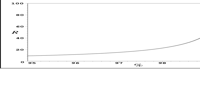
Figure 2: Typical growth of the ratio $R={B_{1,2}}/{B^{\rm sph}}$, Eq. (29), during the late stages of the collapse. The horizontal axis measures the percentage of the total pancake collapse according to $(a-a_{0})/a_{0}\times 100\%$ ($a_{0}\leq a\leq 2a_{0}$ for $\delta_{0}=1$).

Finally, we can gain further insight into the relative amplification of anistropically versus isotropically collapsing magnetic fields by rewriting (28) as

$$\frac{B_{1}}{B^{\rm sph}}=\frac{\ell_{1}}{\ell_{3}}\left(\frac{\ell^{\rm sph}}{\ell^{\rm sph}_{0}}\right)^{2}=\frac{\ell_{1}}{\ell_{3}}\left(\frac{2}{3}+\frac{\ell_{3}}{3\ell_{1}}\right)^{2}\,,$$ (30)

where we have also used Eqs. (15), (26), (27), and linear initial conditions for two initially spherical fluid elements. This relation shows that the ratio ${B_{1}}/{B^{\rm sph}}$ grows almost linearly with the eccentricity of the pancake $\ell_{1}/\ell_{3}$, independent of initial conditions.

4 Conclusions

Protogalactic clouds do not collapse isotropically: in any realistic situation one expects small anisotropies in the initial velocity distribution, which will be amplified as CDM collapse progresses. We used the Zel’dovich approximation to investigate the effects of such gravitational anisotropy on the evolution of a seed magnetic field frozen into the baryon fluid. We considered the mildly nonlinear regime and ignored the magnetic backreaction on the baryons as well as the relative velocity between baryons and CDM. The CDM dominates the collapse and the gravitational anisotropy that amplifies the magnetic field. Our qualitative analysis shows that, as a generic result of the anisotropy of the collapse, the field effectively “loses” one of its components and is confined in the plane of the pancake. Although tidal forces are generally expected to change the orientation of the galactic plane relative to the pancake, our qualitative picture is consistent with magnetic field observations in numerous spiral and disk galaxies. More quantitatively, our results show a much more efficient magnetic amplification in a shearing rather than in a shear-free collapse. This analytical result agrees with numerical simulations of shear and tidal effects on the evolution of magnetic fields in galaxies and galaxy clusters. Taken together, these results indicate that, when the anisotropic effects of CDM collapse are taken into account, the magnetic strengths observed in galaxies today could have originated from seeds considerably weaker than previous estimates.

References

- [Barrow & Gotz 1989] Barrow, J.D. and Gotz, G., 1989, Class. Quantum Grav. 6, 1253
- [Barrow & Subramanian 1998] Barrow, J.D. and Subramanian, K., 1998, Phys. Rev. D 58, 083502
- [Bruni 1996] Bruni, M., 1996, in Mapping, Measuring and Modeling the Universe, ASP Conference Series, eds. P. Coles, V.J Martinez, M.J. Pons-Borderia, Vol. 94
- [Buchert 1996] Buchert, T., 1996, in Proc. International School of Physics Enrico Fermi, Course CXXXII: “Dark Matter in the Universe”, Varenna 1995, eds. S. Bonometto, J. Primack, A. Provenzale ( IOP Press, Amsterdam)
- [Dolag et al 1999] Dolag, K., Bartelmann, M. and Lesch, H., 1999, A & A, 348, 351
- [Dolag et al 2002] Dolag, K., Bartelmann, M. and Lesch, H., 2002, A & A, 387, 383
- [Ellis 1971] Ellis, G.F.R., 1971, in General Relativity and Cosmology, ed. R.K. Sachs, Academic, NY, p. 104
- [Ellis & Tsagas 2002] Ellis, G.F.R. and Tsagas, C.G., 2002 (preprint astro-ph/0209143)
- [Evans & Fennelly 1985] Evans, C.R. and Fennelly, A.J., 1985, Astrophys. Space Sci., 109, 15
- [Grasso & Rubinstein 2001] Grasso, D. and Rubinstein, H.R., 2001, Phys. Rep. 348, 163
- [Han & Wielebinski 2002] Han, J-L. and Wielebinski, R., 2002, Chin. J. Astron. Astrophys. 2, 293
- [Kronberg 1994] Kronberg, P.P., 1994, Rep. Prog. Phys. 57, 325
- [Matarrese 1996a] Matarrese, S., 1996a, in Proc. International School of Physics Enrico Fermi, Course CXXXII: “Dark Matter in the Universe”, Varenna 1995, eds. S. Bonometto, J. Primack, A. Provenzale ( IOP Press, Amsterdam)
- [Matarrese 1996b] Matarrese, S., 1996b, in The Universe at High-z, Large Scale Structure and the Cosmic Microwave Background, eds. E. Martinez-Gonzalez, J.L. Sanz. Lecture Notes in Physics (Springer-Verlag, Berlin)
- [Nusser et al 1991] Nusser, A., Dekel., A., Bertshinger, E. and Blumenthal, G.R., 1991, Ap. J. 379, 6
- [Padmanabhan 1993] Padmanabhan, T., 1993, Structure Formation in the Universe (Cambridge Univeristy Press, Cambridge)
- [Papadopoulos & Esposito 1982] Papadopoulos, D. and Esposito F.P., 1982, Astrophys. J. 257, 10
- [Roettiger et al 1999] Roettiger, K., Stone, J.M. and Burns, J.O., 1999, Astrophys. J., 518, 594
- [Ruzmaikina & Ruzmaikin 1971] Ruzmaikina, T.V. and Ruzmaikin A.A., 1971, Soviet Astron., 14, 963
- [Shandarin & Zel’dovich 1989] Shandarin, S.F. and Zel’dovich, Ya.B., 1989, Rev. Mod. Phys. 61, 185
- [Tsagas & Barrow 1997] Tsagas, C.G. and Barrow, J.D., 1997, Class. Quantum Grav. 14, 2539
- [Tsagas & Maartens 2000] Tsagas, C.G. and Maartens, R., 2000, Phys. Rev. D 61, 083519
- [Wasserman 1978] Wasserman, I., 1978, Ap. J. 224, 337
- [Widrow 2002] Widrow, L.M., 2002, Rev. Mod. Phys., 74, 775
- [Zel’dovich 1970] Zel’dovich, Y.B., 1970, Astrophysica 6, 319
- [Zel’dovich et al 1983] Zel’dovich, Ya.B., Ruzmaikin, A.A. and Sokoloff, D.D., 1983, Magnetic Fields in Astrophysics, Gordon and Breach, NY