A Simple Prediction on the Surface Density of Galaxies at $z\simeq 6$

Abstract

Systematic surveys are being proposed to discover a significant number of galaxies at $z\simeq 6$, which is now suggested as the epoch when the reionization era of the Universe ends. To plan such surveys, we need a reasonable expectation of the surface density of high redshift galaxies at different flux limits. Here we present a simple prediction of the surface density of $5.5\leq z\leq 6.5$ galaxies in the optical regime, $extrapolating$ from what is already known about galaxies at $z\simeq 3$. This prediction is consistent with the results of nearly all known searches for objects at $z\simeq 6$, giving confidence that we may use it to plan optimal combination of survey depth and sky coverage in searching for such objects. We suggest that the most efficient strategy with existing ground-based facilities is to do medium-depth ($m_{AB}\simeq 24.0$ – $24.5$ mag), wide-field (a couple of square degrees) survey using a wide-field camera at a 4m-class telescope. As the predicted surface density at this brightness level is very sensitive to the value of $L^{*}$, the result of such a survey can be easily used to constrain the luminosity evolution from $z\simeq 3$ to 6.

1 Introduction

In the last several years, our knowledge about the Universe at high redshift has been gradually extended to $z\simeq 6$. As of today, five galaxies at $z>5.5$ (Weymann et al. 1998; Hu et al. 1999, 2002; Dawson et al. 2001) and four quasars at $z>5.5$ (Fan et al. 2000, 2001) have been spectroscopically confirmed. The complete Gunn-Peterson trough detected in the $z=6.28$ SDSS quasar by Becker et al. (2001) and further investigation (Fan et al. 2002) led these authors to tentatively identify the end of reionization epoch of the Universe at $z\simeq 6$. Thus the assessment of $z\simeq 6$ galaxy number counts at different brightness levels will have a very direct cosmological impact, since it will quantify the number density of UV-emitting objects that are the physical cause of the reionization. Several systematic surveys aimed at discovering a significant number of $z\simeq 6$ galaxies have now been proposed and are being carried out. To make such surveys efficient, we need to have a rough idea of the surface density of galaxies at $z\simeq 6$. There are a few theoretical predictions on the surface density of galaxies at high redshifts, either based on N-body simulations (cf. Weinberg et al. 1999, 2002) or based on semi-analytic formalisms (cf. Robinson & Silk 2000). However, those predictions are more qualitative than quantitative at this point, because they either are limited by finite volume and finite resolution, or have to rely on several parameters which remain very uncertain in the absence of significant amounts of actual data. Thus one may prefer not to base survey plans directly on such predictions at the moment.

In this paper we present a simple, observational approach. We may $assume$ a reasonable luminosity function for galaxies at $z\simeq 6$ by $extrapolating$ the known results at $z\simeq 3$, which is the highest redshift where the luminosity function of galaxies has been quantified over a wide enough brightness range (Steidel et al. 1999). We will use existing data at $z$${}_{>}\atop{{}^{\sim}}$5 to constrain the normalization of this $extrapolated$ luminosity function. Once the $z\simeq 6$ luminosity function is estimated in this way, the surface density can be calculated in a straightforward manner, $i.e.$, by numerically integrating the luminosity function over the volume occupied by unit sky-coverage in the redshift bin of interest. In §2, we present the details of such a surface density prediction over the range $5.5\leq z\leq 6.5$. We compare our prediction to all the available observations in §3. Comparison to two theoretical models is made in §4. A summary is given in §5.

2 The Predicted Surface Density of Galaxies at $5.5\leq z\leq 6.5$

2.1 The Extrapolated Luminosity Function

We start with the $z\simeq 3$ luminosity function from Steidel et al. (1999), who merged the ground-based and the HDF-N Lyman-break galaxy samples. Since the $z\simeq 3$ sample used in Steidel et al. (1999) was selected based on the Lyman-break signature in the SED of galaxies, our approach makes the implicit assumption that galaxies at higher redshifts also manifest themselves by the Lyman-break feature. Because the line-of-sight intervening H I absorption is more severe at higher redshifts and the effective break moves from the 912Å Lyman limit to the $Ly\alpha$ line at 1216Å (cf. Madau 1995), one can expect that the Lyman-break signature is even stronger, therefore our assumption is likely valid. However, there might exist a different type of galaxy whose UV-photons are completely absorbed by dust, like the ultraluminous infrared galaxies that are known to exist at lower redshifts. There is no Lyman-break for such galaxies, since they have essentially zero flux from the UV to the optical range. Our predictions neglect these objects, because they are also absent from the Lyman-break samples at $z\simeq 3$. Since we deal with the emitted UV, such objects will not affect our conclusions.

The details of the luminosity function extrapolation from $z\simeq 3$ to $z\simeq 6$ depend on the adopted cosmological model. Different cosmological parameters will change the apparent magnitude of an object with a given intrinsic brightness, and will also affect the physical volume corresponding to a given sky coverage. We consider three cosmological models, namely, a flat universe without cosmological constant ($\Omega_{M}=1$ and $\Omega_{\Lambda}=0$), a flat, low mass universe with $\Omega_{M}=0.3$ and $\Omega_{\Lambda}=0.7$, and an open universe without cosmological constant ($\Omega_{\Lambda}=0.2$ and $\Omega_{\Lambda}=0$). For simplicity, we denote the three models by their $\Omega_{M}$ and $\Omega_{\Lambda}$ values as the (1, 0), (0.3, 0.7), and (0.2, 0) models, respectively. Throughout the paper we use a Hubble constant of $H_{0}=65\,km\ s^{-1}\ Mpc^{-1}$. All the quoted magnitudes are AB magnitudes and, unless noted otherwise, refer to the 1400 – 1500Å spectral range in the rest-frame.

The luminosity function of $z\simeq 3$ galaxies of Steidel et al. (1999; see their section 4.3) is a Schechter function of the form $\Phi(L)=(\Phi^{*}/L^{*})(L/L^{*})^{\alpha}exp(-L/L^{*})$. The $L^{*}$ galaxies at this redshift have $\mathcal{R}$-band apparent magnitude of $m^{*}=24.48$ mag. At $z=3.04$ (the median redshift for Steidel et al.’s sample), this $m^{*}$ value corresponds to $M^{*}=-20.37$, $-21.23$ and $-21.31$ mag in the (1, 0), (0.3, 0.7) and (0.2, 0) models, respectively. The $\mathcal{R}$-band has central wavelength of $\lambda_{0}=6930$Å, or $\sim 1700$Å in the rest-frame at $z\simeq 3$. Since the SED of a young non-dusty galaxy in $f_{\nu}$ is essentially flat from 1400 – 1700Å, these magnitudes apply to the 1400 – 1500Å range as well. As a first approximation, we also assume that there is no significant luminosity evolution for galaxies from $z\sim 3$ to $5.5\leq z\leq 6.5$, such that $L^{*}$ galaxies at $5.5\leq z\leq 6.5$ still have the above mentioned absolute magnitudes. Possible evolution effects will be discussed in §5. We noticed that Steidel et al. (1999) made a similar assumption in comparing the ground-based + the HDF-N sample at $z\simeq 4$ to its counterpart at $z\simeq 3$, concluding that the observed $z\simeq 4$ galaxy distribution was completely consistent with such an assumption at the bright end, and within a factor of two at the faint-end. In fact, they suggested that the faint end mismatch was due to the genuine structure in the small HDF-N field, rather than a true luminosity function discrepancy. We use continuum magnitudes, ignoring the possible contribution of $Ly\alpha$ line emission, for two reasons: 1) only 50% of the galaxies in the sample of Steidel et al. are $Ly\alpha$ emitters, although there was a strong bias in favor of such objects in the spectroscopic identification, and 2) the vast majority of those $Ly\alpha$ emitters are weak in $Ly\alpha$ strength. We assume a slope of $\alpha=-1.6$, but our conclusions are insensitive to the exact value.

Next we choose a normalization to fix the luminosity function, which amounts to allowing density evolution. Observationally, this can be done by adjusting $\Phi^{*}$ such that the calculated surface density, either differential or cumulative, matches the availible observations. This is difficult in our case, since there is no precise observed value to be used. There are only four published $z>5.5$ galaxies with spectroscopic information. These are the z=5.60 galaxy in the HDF-N (Weymann et al. 1998), the z=5.74 galaxy in the Hawaii Survey Field SSA22 (Hu et al. 1999), and the z=5.767 and z=5.631 galaxies in the HDF-N flanking fields (Dawson et al. 2001). Statistically, these results are inadequate for the purpose of normalization, because their selection is not readily quantifiable. Nevertheless, we can still make a rough estimate of the cumulative surface densities of $z\geq 5.5$ galaxies in the well-studied HDF-N and use this value as our normalization. We consider two cases: a cumulative surface density of 1.37 per arcmin² and 0.11 per arcmin², both to a limit $m_{AB}=27.0$ mag. The former case (high normalization) is equivalent to $one$ $z\geq 5.5$ galaxy per NIC-3 field (cf. Thompson et al. 1999) and the later one (low normalization) is equivalent to $one$ such galaxy per WFPC2 HDF coverage. Note that $m_{AB}=27.0$ mag is $not$ the magnitude of this z=5.60 galaxy, but an estimate of the selection limit for a galaxy at $z\geq 5.5$ as observed at 9100 – 9800Å. This galaxy is $not$ a $Ly\alpha$ emitter, confirming that the magnitude in our prediction should be taken as referring to the continuum brightness level rather than including this emission line.

2.2 The Predicted Surface Densities

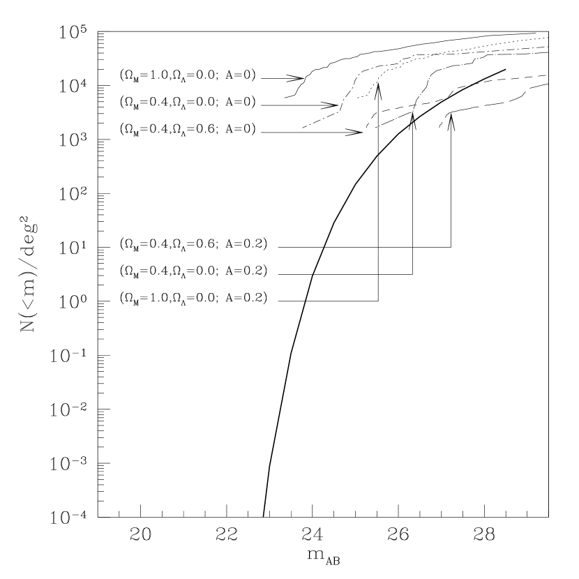
Cumulative surface densities can now be calculated by numerically integrating the luminosity function over the volume occupied by unit sky coverage in the range $5.5\leq z\leq 6.5$. Fig. 1 shows these results, where the cumulative surface density is presented as the total number of galaxies per deg², whose brightness is brighter than a specified apparent AB magnitude. The predictions for the (1, 0), (0.3, 0.7) and (0.2, 0) models are plotted in solid, long-dashed and short-dashed lines, respectively. Thick lines are used for the high normalization case, while thin lines are used for the low normalization one. The absolute magnitude scales are labeled on top of the figure, from bottom to the top for the (1, 0), (0.3, 0.7) and (0.2, 0) models, respectively. The $M^{*}$ values for these models are labeled in the legend in the parenthesis together with the corresponding apparent magnitudes, and are also indicated along the absolute magnitude scales at the top by upward arrows. Numerical results are presented in Table 1, where the number density is listed as number of galaxies per arcmin² for straightforward use in planning future observations.

Figure 1: The cumulative surface density predictions of $z\simeq 6$ galaxies in the $5.5\leq z\leq 6.5$ redshift bin, presented as the total number of galaxies per deg² whose brightness is brighter than a specified apparent magnitude (defined around 9100 – 9800Å  on the AB scale). The results for the (1, 0), (0.3, 0.7) and (0.2, 0) models are plotted in solid lines, long-dashed lines and short-dashed lines, respectively. The high and low normalization cases are plotted in thick and thin lines, respectively. The “$+$” labels mark the positions where the HDF-based normalizations are placed. The corresponding absolute magnitude scales are labeled on top of the figure, from bottom to the top for the (1, 0), (0.3, 0.7) and (0.2, 0) models. The $M^{*}$ values in these three models are given in the legend together with the corresponding apparent magnitude scales, and are also marked with the upward arrows on the scales. The upper limit derived from the preliminary data of our survey is indicated by the thick downward arrow, while the lower limit derived from Hu et al. (1999) is labeled by the thick upward arrow. The indirect bright-end upper-limit inferred from the hosts of the SDSS $5.5\leq z\leq 6.5$ quasars is indicated by “$\bot$” from the left to right for (1, 0), (0.3, 0.7) and (0.2, 0) models, respectively.

3 Consistency Check from Limited Observations

As a minimal consistency check, we compare our predictions to the limited (direct and indirect) observations in hand for galaxies at $z\simeq 6$.

3.1 The Intermediate Brightness Level   ($23<m_{AB}<24$ mag)

Our group has started a multi-color search for $z\simeq 6$ object, aimed at constraining the luminosity function at this intermediate brightness level. Four medium-band filters, namely, $m(802nm)$, $n(848nm)$, $o(919nm)$ and $p(974nm)$, are used in this survey. These are the four reddest of our 15 medium-band filters which cover the entire $300$ – $1000\,nm$ range, and are designed to avoid the brightest and most variable night-sky lines to yield dark background and fringe-free imaging. These four filters are ideal for discriminating the Lyman-break signature in the SED of galaxies at $5.5\leq z\leq 6.5$. Specifications of these filters can be found in the series of papers of the BATC (Beijing-Arizona-Taiwan-Connecticut) Survey, whose filters are essentially the same but smaller in physical size (Fan et al. 1996; Shang et al. 1998; Zheng et al. 1999; Yan et al. 2000).

Our medium-band data so far allow us to put a meaningful constraint on the luminosity function at $z\simeq 6$. In our pilot run in June 2000, we observed a $35^{\prime}\times 35^{\prime}$ area around the HDF-South in the reddest three bands ($n$, $o$ and $p$), using the MOSAIC-II array mounted at the CTIO-4m telescope. Details of the observation will be presented elsewhere (H. Yan et al., in preparation). To summarize, we reached AB magnitudes of $n(848nm)$ = 23.2, $o(919nm)$ = 23.5 and $p(974nm)$ = 23.0 mag at 5-$\sigma$ with $>50\%$ completeness, and used these images to search for drop-outs at $z\simeq 6$. We found three candidates which were absent from the $n(848nm)$-band image but prominent in the $o(919nm)$-band. However, since these objects are also very faint in the $p(974nm)$-band, imaging in bluer passbands is needed to confirm their nature. Two out of these three objects lie within the broad band $UBVRI$ CTIO-4m BTC images of Palunas et al. (2000), whose survey field has about a $15^{\prime}\times 15^{\prime}$ overlapping region with ours. These two drop-outs are both clearly visible on the BTC $R$-band and shortward images, but not on the I-band image. Thus these two objects are most likely lower redshift interlopers, possibly $z=2.3$ quasars with $MgII$ redshifted to $\sim$ 9100Å. This meant that at best only one positive candidate remained that could be at $z\simeq$ 5.5–6.5.

Based on these results, we can put a safe upper limit to the cumulative number density of $5.5\leq z\leq 6.5$ objects as one object in $35^{\prime}\times 35^{\prime}$ down to the flux limit of $m_{AB}=23.5$ mag. This upper limit is indicated on Fig. 1 by an downward arrow, and is consistent with both high and low normalization cases in our prediction.

3.2 The Faint End   ($m_{AB}>25$ mag)

A lower limit at this brightness level can be obtained from the $z=5.74$ galaxy of Hu et al. (1999), assuming that its single strong emission line identification is reliable. The galaxy’s $Z$-band magnitude (free of the emission line), which is similar to the SDSS $z^{\prime}$-band magnitude, is 25.5 mag. Since their survey area is about $390\arcsec\times 280\arcsec$, a simple lower limit estimation is $log(N)=2.07/\deg^{2}$ to $m=25.5$ mag. This lower limit is indicated on Fig. 1 as “$\bot$”, and fits with our high normalization case but not with the low one.

Unfortunately, the two $z>5.5$ galaxies of Dawson et al. (2001) cannot be used as a direct constraint to the luminosity function, since no continuum magnitude was given for either of the two. However, because their $I_{AB}$ magnitudes are all fainter than 25, their result is at least not in conflict with our estimates above.

3.3 Indirect Result at the Bright End   ($m_{AB}\sim 23$ mag)

Finding any $z\simeq 6$ galaxies at these bright levels would require a SDSS-like all-sky survey, but extending at least one magnitude deeper, which is a daunting, if not impossible, task with any existing facilities. However, we can get some information in this regime by using quasar host galaxies as the tracers of the entire galaxy population. To the extent that quasar hosts can be taken as representatives of galaxies, it is possible to obtain a reasonable, although indirect, bright-end lower limit if the hosts luminosity of the known $z\simeq 6$ quasars can be obtained. It has been long suggested that there is a linear relation between the quasar luminosity and the $minimum$ luminosity of its host galaxy (cf. McLeod & Rieke 1995), which can be understood in the sense that a more luminous host galaxy is required to fuel a more luminous quasar. Thus there might be a similar relation between the luminosity of the quasar and that of its host at higher redshift. Such a relation would give a luminosity function constraint from the four $z>5.5$ quasars known, all discovered by SDSS in $\sim$ 1500 deg² of survey area (Fan et al. 2000, 2001).

We construct such a relation from Bahcall et al. (1996), who imaged twenty nearby ($z<0.3$) luminous quasars with HST, and obtained their host luminosities. A simple fit to their data gives $M_{host}=0.425\times M_{qso}-11.82$ ($rms=0.38$ mag). Using this formula, we found that the host luminosities of the four $z>5.5$ SDSS quasars were almost identical. Their average absolute magnitude at around rest-frame 1400Å is $M=-23.1$, $-23.5$ and $-23.7$ mag ($rms$ $\sim$ 0.2 mag) in the (1, 0), (0.3, 0.7) and (0.2, 0) universe, respectively, which correspond to apparent magnitudes of 22.8, 23.4 and 23.6 mag, respectively, at $z=6$. The AGN unification scheme implies that if an AGN is detected, statistically there must be two or more galaxies which also harbor AGN activity, which cannot be detected because obscuring matter in the surrounding torus largely blocks our view. In other words, since there are four $z>5.5$ quasars detected in $\sim$ 1500 deg², the total number of $z>5.5$ galaxies (including the four quasar hosts) is at least 12, implying a number density of $log(N)\geq 2.10/\deg^{2}$ at the above mentioned brightness levels. As indicated above, this number should be taken as a lower limit, because there could be some galaxies as luminous as the quasar hosts, but lack a massive central black hole and thus cannot be traced by AGN. This indirect constraint is shown by the upward arrow in Figure 1.

There are two major uncertainties on this bright-end constraint. One is the effect of quasar luminosity evolution. The above linear relation between the hosts and the quasars is inferred from a local sample, yet we apply it to $z\simeq 6$. Typical quasar luminosities have been shown to evolve with redshift, as $(1+z)^{\beta}$ with $\beta=2.5$–4 for $z<2.5$. This indicates that quasars may have once been brighter with respect to their hosts than we see today. In other words, the hosts of the $z\simeq 6$ quasars could be fainter than we estimated here, and therefore the limits shown in Fig. 1 could be moved more to the right. However, since it is almost impossible to obtain a quantitative estimate about the amplitude of such a shift, we just leave the derived constraint as it is now. Another issue is whether quasar hosts are fair representatives of field galaxies, and therefore whether the above bright-end limit is meaningful. Bahcall et al. (1996) speculated that the quasar hosts might not fit a Schechter function and might be 2.2 mag brighter than field galaxies. However, their suggestion was based on a volume-limited sample, which is clearly not the case for their luminous quasar sample. Furthermore, galaxy evolution clearly cannot be neglected in comparing results from $z\approx 0.2$ to $z\approx 6$. Net evolution of the hosts would move this constraint to higher luminosity, running counter to the effect of quasar luminosity evolution.

Even in the light of these caveats, we believe that the bright-end constraint indicated by the SDSS $z>5.5$ quasars is useful. In fact, the (1, 0) model, either high or low normalization, and the low normalization case of the (0.2, 0) model, are clearly not consistent with this constraint. The high normalization case of both the (0.3, 0.7) and (0.2, 0) models, on the other hand, are perfectly consistent with this constraint. The low normalization case of the (0.3, 0.7) model is barely consistent with this constraint. Thus, the mere detection of four quasars at $z>5.5$ implies a rather high normalization to the counts and luminosity function of galaxies at these redshifts.

3.4 Recent Narrow-band Search

The only reported data which seem hard to reconcile with our prediction are from the $z=5.7$ $Ly\alpha$ emitter search of Rhoads & Malhotra (2001), who used two narrow-band filters to look for $Ly\alpha$ emission. They reported 18 robust $z$=5.7 $Ly\alpha$ emitters in 0.36 deg² to a 5-$\sigma$ survey limit of $m_{AB}$=24.8 mag (average for both bands), and discussed cosmological implications of this result. Although these objects have not yet been spectroscopically confirmed, we compared our prediction against this result for the sake of completeness. For simplicity, we only compare it against our high normalization (0.3, 0.7) model.

To make such a comparison, we need both their cumulative number density corrected for the survey volume and the 9100–9800Å continuum magnitudes of their objects. The two narrow-band filters that they used, $815nm$ and $823nm$, are both 75Å wide and can only pick up $Ly\alpha$ emission from $z=5.70$ – 5.78. The co-moving volume of their survey is $3.27\times 10^{5}\,Mpc^{3}$ for their 0.36 deg² sky coverage. Our model uses $5.5\leq z\leq 6.5$, giving a co-moving volume of $3.96\times 10^{6}\,Mpc^{3}$ for the same sky coverage. Since their survey volume is only 8% of this, the 18 objects that they detected should only account for 8% of the total galaxies in our prediction. In other words, if the 18 objects were taken at their face values, the total number of galaxies that our model would predict is 225 in our volume at $5.5\leq z\leq 6.5$. Furthermore, the objects they found are believed to be strong $Ly\alpha$ emitters. Although spectroscopic identification is strongly biased in favor of such objects, past studies indicate that they are only a minority of the entire population. If the $z\simeq 3$ Lyman-break galaxy result of Steidel et al. (1999) is universal only $\sim 25\%$ of the Lyman-break galaxies have $Ly\alpha$ emission strong enough to be picked up in such narrow-band searches. This means the total number of $z\sim 5.7$ galaxies inferred from Rhoads & Malhotra’s result is about 72, and thus the total number of objects that our model would predict is 900. Translated into number density, it amounts to 0.694 per arcmin². Note that we assume their 18 objects form a complete sample down to their detection limit, which is possibly not the case. If we made a correction for their survey incompleteness, the inferred number density would be even higher.

The continuum magnitudes of these objects were not explicitly given in their paper, therefore we use the equivalent width of the weakest object to estimate their survey limit in terms of continuum magnitude. Using the numbers from Figure 1 of Rhoads & Malhotra (2001), we find that the weakest emitter has $f_{\nu}(line)=0.48$ $\mu Jy$ in the line, or equivalently $m_{AB}(line)=24.70$ mag, almost approaching their detection limit. Using the approximation that $f_{\nu}(line)/f_{\nu}(continuum)=(W/\Delta\lambda)+1$, where $W$ is the equivalent width and $\Delta\lambda$ is the bandwidth, we find that $f_{\nu}(continuum)=0.23\mu Jy$, or $m_{AB}(continuum)=25.50$ mag. At this brightness level, our model gives the cumulative surface density of only 0.138 per arcmin².

This comparison shows that Rhoads & Malhotra’s result gives a factor of five times higher cumulative number density as our prediction does. Stated differently, if their result were used as our normalization at $m_{AB}=25.50$ mag, the number of $z\simeq 6$ objects in the HDF-N would be much higher ($>$ 6 times) than what have been found. Since the Rhoads & Malhotra’s objects still need spectroscopic identification to judge their real nature, we shall not go further than pointing out that there is a discrepancy.

Figure 2: Comparing our estimates with the N-body simulation prediction of Weinberg et al. (2002). The high normalization case of our (0.3, 0.7) model is plotted as the thick solid line. The thin lines of different types are the predictions of Weinberg et al. (2002), reproduced by reading off the numbers from their Figure 8 and following the converting procedures given by their paper. Two flavors of these models are shown: one is without any dust extinction ($A=0$ at around 1500 Å), and the other has a dust extinction of $A=0.2\,mag$. Note how large the differences in the number count predictions are with only slight differences in the assumed dust extinction alone. Obviously only the (0.4, 0.6) model (LCDM) does not conflict with the HDF-N result.

4 Compared with Theoretical Models

We compare our estimates with the hierarchical N-body modeling results of Weinberg et al. (2002) in Fig. 2. The thick solid line is our (0.3, 0.7) high normalization estimate. The thin lines of different types are the predictions of Weinberg et al. (2002), reproduced by reading off the numbers from their Figure 8 and following the converting procedures given by their paper. Only three of their models are reproduced here, namely, CCDM, LCDM and OCDM, which correspond to $(\Omega_{M},\Omega_{\Lambda})=(1,0)$, $(0.4,0.6)$ and $(0.4,0)$, respectively. Their choices of $\Omega_{M}$ and $\Omega_{\Lambda}$ are slightly different from ours, but the effects of these on the global trends are only marginal. Two flavors of these models are shown: one is without any dust extinction ($A=0$ at restframe 1500Å), and the other is with $20\%$ dust extinction ($A=0.2$ mag). Note that the count predictions can differ widely solely due to different assumptions about the internal extinction. Obviously only the (0.4, 0.6) model (LCDM) does not conflict with the HDF-N result as summrized in our Fig. 1 and §2.1. Furthermore, nearly all those models predict unrealistically high surface density at mAB$\leq 24.5$ mag, which is caused by the finite resolution in the simulations. Trading volume for finer resolution (Weinberg et al. 1999), their LCDM result would give a more realistic surface density at the bright end, but again would predict too high a value at the faint end.

It is also interesting to do a comparison among the theoretical predictions. For example, we can compare the result derived from Weinberg et al. (2002) as shown in Figure 2 with the semi-analytic result of Robinson & Silk (2000) as shown in their Figure 3. A direct, quantitative comparison is not meaningful, since the result here is for $z=6$ while the highest redshift given in Robinson & Silk’s Figure 3 is $z=5$, and their choices of $\Omega_{M}$ and $\Omega_{\Lambda}$ are slightly different. But we can still compare the global trends, which show obvious differences. In Robinson & Silk’s semi-analytic formalism, the (1, 0) model gives the lowest galaxy counts, the (0.3, 0.7) lies in between, and the (0.2, 0) one gives the highest galaxy counts. They explained such trends as the result caused by the dominant effects of the different volume element $dV/dz$ and the growth factor $G$ in different cosmologies. A lower-density universe always has higher $dV/dz$ and larger $G$, and the combination of these two factors dominates the competing effect of the larger luminosity distance which makes objects fainter in such a universe. On the other hand, Weinberg et al.’s (1, 0) model yields the highest counts, (0.4, 0.6) yields the lowest counts, and (0.4, 0) is in between. Notice that in our approach (1, 0) gives the highest counts, (0.3, 0.7) is in between, and (0.2, 0) gives the lowest counts. It is possible that the reasoning of Robinson & Silk (2000) might only be partially true, and that other effects which they did not consider might actually be important. For example, if the luminosity of $L^{*}$ galaxies in a high-density universe is brighter than that can be produced from their current model, the number counts in different cosmologies might have a different behavior from that shown in their paper.

5 Discussion and Conclusion

5.1 The Effect of Luminosity Evolution

The most crucial assumption made in our prediction is that the luminosity evolution from $z\simeq 3$ to 6 is not significant, so that the value of $L^{*}$ at around restframe 1400Å is still the same at $z\simeq 6$ as at $z\simeq 3$. However, there are several possibilities where this condition could break down. There are at least two major competing effects which are relevant. One possibility is that the merger/star-forming rate could be lower at $z\simeq 6$, and so would bring down the value of $L^{*}$. On the other hand, both dust extinction and metallicities could be lower at earlier epochs as well, which would make $L^{*}$ brighter. Since these effects tend to cancel each other out, we believe that to first order our assumption is reasonable. Needless to say, the reality could be more complicated that what we assumed. For example, it has been suggested that $L^{*}$ evolves mildly in the form $L^{*}\propto(1+z)^{\beta}$, where $\beta$ varies from $-1$ to $-1.5$ ($e.g.$ Lanzetta et al. 1999). As described below, the surface density at the bright end is extremely sensitive to the $L^{*}$ value. Therefore, a direct comparison between this simple prediction, which serves as a first approximation, and any future observations can give quantitative estimates on how the luminosity evolves from $z\simeq 3$ to 6. For the sake of completeness, here we discuss how the possibilities mentioned above would affect our prediction.

The time interval between $z=3$ and $z=6$ is about 1.28 Gyr in a $\Omega_{M}=0.3$, $\Omega_{\Lambda}=0.7$, and $H_{0}=65$ universe, and is likely only sufficient to allow one major merger ($cf.$ Makino & Hut 1997). Hence a higher merger rate alone would at most make $L^{*}$ at $z\simeq 3$ twice as bright as at $z\simeq 6$. On the other hand, a higher merger rate would certainly make star formation rate higher, and this would further contribute to the luminosity. The later effect, however, has not yet been well quantified. As a very rough estimation, the higher star formation rate could contribute another factor of few in increasing $L^{*}$ at $z\simeq 3$. Thus the overall effect of merger/star formation rate difference would make $L^{*}$ at $z\simeq 3$ four to six times as bright as at $z\simeq 6$, or a difference of 1.5–2 mag.

The dust content and metallicities are likely to increase from $z\simeq 6$ to 3, and these would affect $L^{*}$ in the opposite way. For example, one of the more reddened object in Steidel et al.’s sample, MS 1512-cB58, is quoted having $E(B-V)\simeq 0.3$ mag (Pettini et al. 2001). Assuming the extinction law of Calzetti et al. (2000), this number translates to $A_{1400\AA}\simeq 2.6$ mag. This means the galaxies at $z\simeq 6$ could get brighter by 2.6 mag at most, if dust extinction is largely absent at this redshift. The metallicity of galaxies at large redshift is again very hard to quantify and seems to have a wide spread ($c.f.$ Nagamine et al. 2001); but in any case, it is not likely that this effect would contribute more than 0.5 mag increase in brightness at $z\simeq 6$ at around rest-frame 1400 Å.

To investigate how the surface density could be affected by the luminosity evolution, we also calculated the surface densities for different $M^{*}$ values. Specifically, we looked at the limits of the $M^{*}$ value where the high normalization case starts to conflict with the known constraints, and where the low normalization case begins to be consistent with those constraints. Since $\Omega_{M}=0.3$ and $\Omega_{\Lambda}=0.7$ are currently the most widely accepted values, for the sake of simplicity, we will only discuss our (0.3, 0.7) model here. In the high normalization case, if $M^{*}$ is brighter by more than 0.7 mag at $z\simeq 6$, the predicted counts will conflict with our CTIO upper limit. If $M^{*}$ is fainter by only 0.3 mag at $z\simeq 6$, on the other hand, the counts will conflict with the lower limit derived from the SDSS QSO hosts by more than a factor of two. In the low normalization case, $M^{*}$ needs to be brighter by at least 2.0 mag to make the counts consistent with the Keck lower limit. In the mean time, however, such $M^{*}$ value makes the counts inconsistent with our CTIO upper limit, overpredicting the counts by a factor of two. This situation further confirms that the low normalization case can be rejected.

5.2 Summary

We present a simple empirical approach to predict the galaxy surface density at $z\simeq 6$, which $extrapolates$ the known luminosity function of $z\simeq 3$ galaxies to $z\simeq 6$. Our approach is based on only two observational results, namely, the observed luminosity function of $z\simeq 3$ Lyman-break galaxies and the number of $5.5\leq z\leq 6.5$ galaxies in the HDF-N, and the assumption that there is no $strong$ luminosity evolution for galaxies from $z\simeq 3$ to $z\simeq 6$. The biggest uncertainty in our estimates comes from the normalization, $i.e.$, the actual number density of $z\simeq 6$ galaxies in the HDF-N down to the limit of $m_{AB}$ = 27.0 mag, for which we used one per WFPC-2 field and one per NIC-3 field as our low and high normalization, respectively. We checked our results against the constraints derived from all known observations. It seems that the low normalization case can be rejected. The high normalization case, on the other hand, is consistent with most constraints if the prediction is made in the (0.3, 0.7) or (1, 0) models. The only observation with which our predictions do not agree is the narrow-band $z=5.7$ $Ly\alpha$ emitter result reported by Rhoads & Malhotra (2001), whose number density is at least 5 times higher than our prediction. If their result were used as the normalization, it would suggest that the number of $z\geq 5.5$ objects in the HDF be at least 6 times as many as actually found. Since these emitters still need future spectroscopic identification to judge their real nature, we conclude that this is only a potential conflict. On the other hand, a direct comparison between our prediction and any future observations can give quantitative estimation on how the luminosity evolves at different epochs, as indicated in the previous section.

To summarize, we believe that our simple approach can be used to plan future surveys, where there will always be compromise between depth and sky coverage. As our prediction indicates, currently the most realistic way to find a significant number of $z\simeq 6$ galaxies with the available ground-based facilities is to do multi-color, medium-depth and wide-field surveys reaching continuum $m_{AB}\sim 24.0$ – $24.5$ mag from 8400Å to the CCD Q.E. cut-off at around 1$\mu m$, and covering a couple of square degrees. There are now several wide-field CCD cameras available at telescopes of sufficient light-gathering power, e.g., the MOSAIC-I/II at the KPNO/CTIO 4m’s, the CFH12K at the CFHT and the Suprime-Cam at the Subaru. Carefully designed surveys at a 4m class telescope could possibly discover a few dozen $L>L^{*}$ $z\simeq 6$ galaxies within a few nights of observation (Yan et al. 2002, in preparation). On the other hand, deep, pencil-beam surveys from the ground are not likely to be very successful even with 8-10m class telescopes. As Table 1 indicated, pencil-beam surveys with a few square arcmin field of view would have to reach at least $m_{AB}=27$ mag in the difficult spectrum regime redder than 8400Å to discover a significant number of such objects. Since at least two bands of observation at similar depth are needed to select drop-out candidates, the telescope time required is very costly if not unrealistic. In the immediate future, it should be possible to use the the Advance Camera for Surveys, which was installed on board HST in Macrh 2002, for drop-out searches to better constrain the luminosity function at $z\simeq 6$. Accessing the faint end of the luminosity function at $z\geq 6$ will be one of the major goals that we will pursue with the Next Generation Space Telescope (NGST) out to redshifts as high $z\simeq 9-10$, and possibly beyond.

Table 1: Number Density Prediction for Galaxies at $5.5\leq z\leq 6.5$

		(1.0,  0.0)		(0.3,  0.7)		(0.2,  0.0)
m	M	$\Sigma$	M	$\Sigma$	M	$\Sigma$
22.00	$-23.91$	2.19e-14	$-24.86$	2.33e-15	$-25.30$	3.02e-20
22.50	$-23.41$	6.83e-10	$-24.36$	1.65e-10	$-24.80$	1.38e-13
23.00	$-22.91$	5.98e-07	$-23.86$	2.42e-07	$-24.30$	2.66e-09
23.50	$-22.41$	5.44e-05	$-23.36$	3.06e-05	$-23.80$	1.76e-06
24.00	$-21.91$	1.17e-03	$-22.86$	8.12e-04	$-23.30$	1.34e-04
24.50	$-21.41$	1.00e-02	$-22.36$	7.95e-03	$-22.80$	2.57e-03
25.00	$-20.91$	4.71e-02	$-21.86$	4.08e-02	$-22.30$	2.04e-02
25.50	$-20.41$	1.50e-01	$-21.36$	1.38e-01	$-21.80$	9.15e-02
26.00	$-19.91$	3.67e-01	$-20.86$	3.51e-01	$-21.30$	2.82e-01
26.50	$-19.41$	7.53e-01	$-20.36$	7.40e-01	$-20.80$	6.77e-01
27.00	$-18.91$	1.37e+00	$-19.86$	1.37e+00	$-20.30$	1.37e+00
27.50	$-18.41$	2.29e+00	$-19.36$	2.32e+00	$-19.80$	2.47e+00
28.00	$-17.91$	3.59e+00	$-18.86$	3.67e+00	$-19.30$	4.09e+00
28.50	$-17.41$	5.40e+00	$-18.36$	5.56e+00	$-18.80$	6.39e+00
		(1.0,  0.0)		(0.3,  0.7)		(0.2,  0.0)
m	M	$\Sigma$	M	$\Sigma$	M	$\Sigma$
22.00	$-$23.91	1.76e-15	$-$24.86	1.87e-16	$-$25.30	2.43e-21
22.50	$-$23.41	5.49e-11	$-$24.36	1.32e-11	$-$24.80	1.07e-14
23.00	$-$22.91	4.80e-08	$-$23.86	1.94e-08	$-$24.30	2.13e-10
23.50	$-$22.41	4.36e-06	$-$23.36	2.46e-06	$-$23.80	1.41e-07
24.00	$-$21.91	9.39e-05	$-$22.86	6.52e-05	$-$23.30	1.07e-05
24.50	$-$21.41	8.03e-04	$-$22.36	6.38e-04	$-$22.80	2.06e-04
25.00	$-$20.91	3.78e-03	$-$21.86	3.28e-03	$-$22.30	1.64e-03
25.50	$-$20.41	1.20e-02	$-$21.36	1.11e-02	$-$21.80	7.35e-03
26.00	$-$19.91	2.95e-02	$-$20.86	2.82e-02	$-$21.30	2.26e-02
26.50	$-$19.41	6.05e-02	$-$20.36	5.94e-02	$-$20.80	5.43e-02
27.00	$-$18.91	1.10e-01	$-$19.86	1.10e-01	$-$20.30	1.10e-01
27.50	$-$18.41	1.84e-01	$-$19.36	1.86e-01	$-$19.80	1.98e-01
28.00	$-$17.91	2.88e-01	$-$18.86	2.95e-01	$-$19.30	3.28e-01
28.50	$-$17.41	4.33e-01	$-$18.36	4.46e-01	$-$18.80	5.13e-01

References

- Bahcall et al. (1997) Bahcall, J. N., Kirhakos, S., Saxe, D. H., & Schneider, D. P. 1997, ApJ, 479, 642
- (2) Calzetti, D. et al. 2000, ApJ, 533, 682
- (3) Dawson, S., Stern, D., Bunker, A. J., Spinrad, H., & Dey, A. 2001, AJ, 122
- (4) Fan, X., et al. 1996, AJ, 112, 628
- (5) Fan, X., et al. 2000, AJ, 120, 1167
- (6) Fan, X., et al. 2001, AJ, 122, 2833
- (7) Fan, X., et al. 2002, AJ, 123, 124
- (8) Hu, E. M., McMahon, R. G., & Cowie, L. L. 1999, ApJ, 502, L9
- (9) Hu, E. M., et al. 2002, ApJ, 568, L75
- (10) Lanzetta, K. M., et al. 1999, in ASP Conf. Ser. 193, The Hy-Redshift Universe: Galaxy Formation and Evolution at High Redshift, ed. A. J. Bunker & W. J. M. van Breugel (San Francisco: ASP), 544
- (11) Madau, P. 1995, ApJ, 441, 18
- (12) McLeod, K. K. & Rieke, G. H. 1995, ApJ, 454, L77
- (13) Makino, J. & Hut, P. 1997, ApJ, 481, 83
- (14) Nagamine, K., Fukugita, M., Cen, R., & Ostriker, J. 2001, ApJ, 558, 497
- (15) Palunas, P., et al. 2000, ApJ, 541, 61
- (16) Pettini, M., et al. 2001, ApJ, 554, 981
- (17) Rhoads, J. E. & Malhotra, S. 2001, ApJ, 563, L5
- (18) Robinson, J. & Silk, J. 2000, ApJ, 539, 89
- (19) Shang, Z., et al. 1998, ApJ, 504, L23
- (20) Steidel, C. C., Adelberger, K. L., Giavalisco, M., Dickinson, M., & Pettini, M. 1999, ApJ, 519, 1
- (21) Thompson, R. I., Storrie-Lombardi, L. J., Weymann, R. J., Rieke, M. J., Schneider, G., Stobie, E., Lytle, D. 1999 AJ, 117, 17
- (22) Weinberg, D. H., Hernquist, L., & Katz N. 2002, ApJ, 571, 15
- (23) Weinberg, D. H. et al. 1999, in ASP Conf. Ser. 191, Photometric Redshifts and the Detection of High Redshift Galaxies, ed. R. Weymann et al. (San Francisco: ASP), 341
- (24) Weymann, R., et al. 1998, ApJ, 505, L95
- (25) Yan, H., et al. 2000, PASP, 112, 691
- (26) Zheng, Z., et al. 1999, AJ, 117, 2757
- (27) Zheng, W., et al. 2000, AJ, 120, 1607