The X-ray luminosities of Herbig-Haro objects

Abstract

The recent detection of X-ray emission from HH 2 and HH 154 with the Chandra and XMM-Newton satellites (respectively) have opened up an interesting, new observational possibility in the field of Herbig-Haro objects. In order to be able to plan further X-ray observations of other HH objects, it is now of interest to be able to estimate their X-ray luminosities in order to choose which objects to observe. This paper describes a simple, analytic model for predicting the X-ray luminosity of a bow shock from the parameters of the flow (i. e., the size of the bow shock, its velocity, and the pre-shock density). The accuracy of the analytic model is analyzed through a comparison with the predictions obtained from axisymmetric, gasdynamic simulations of the leading working surface of an HH jet. We find that our analytic model reproduces the observed X-ray luminosities of HH 2 and HH 154, and we propose that HH 80/81 is a good candidate for future observations with Chandra.

1 Introduction

More than two decades ago, Ortolani & D’Odorico (1980) detected the UV emission of the Herbig-Haro object HH 1 with the International Ultraviolet Explorer (IUE). This observation opened up the new possibility of carrying out ultraviolet observations of HH objects, which resulted in a large number of papers describing results obtained with IUE (see, e. g., Moro-Martín et al. 1996), the Hopkins Ultraviolet Telescope (Raymond et al. 1997) and the Hubble Space Telescope (HST, Curiel et al. 1995).

Very recently, Pravdo et al. (2001) have reported Chandra observations of HH 2 and Favata et al. (2002) have reported XMM-Newton observations of HH 154 which are the first X-ray detections ever of HH objects. Even though HH 2 and HH 154 are detected only in a marginal way, these observations open up the new possibility of analyzing the X-ray properties of HH objects. This is an exciting development in observations of outflows from young stars, because it gives us the possibility of detecting fast, non-radiative shocks which could be associated with the outflows but have not been previously detected. The results of future X-ray observations of HH objects, however, will depend on whether or not other HH objects are bright in the 0.1 - 10 keV window observed by Chandra.

In the present paper, we derive a simple, analytic model which gives the X-ray luminosity of a bow shock as a function of the flow parameters (§2). We then compare this analytic model with predictions obtained from axisymmetric simulations of the leading working surface of a jet (§3) in order to evaluate its accuracy. Finally, in §4 we compare the luminosity predicted from our model with the HH 2 observations of Pravdo et al. (2001), and suggest other objects which appear to be good candidates for future Chandra observations.

2 The analytic model

A simple estimate of the X-ray luminosity of an HH bow shock can be obtained as follows. We first assume that the X-ray luminosity is dominated by the contribution of the free-free emission of hydrogen, and that most of the free-free continuum photons come out in the X-ray wavelength range. Then, the X-ray emission per unit volume is given by the classical formula

$$\Lambda_{ff}={1.85\times 10^{-27}{\rm erg\,cm^{-3}\,s^{-1}}}T^{1/2}n^{2}\,,$$ (1)

where the temperature $T$ and the number density $n$ (of H ions or of free electrons) are in cgs units (see, e. g., Osterbrock 1989, p. 53). In order to evaluate the errors introduced by neglecting the line emission, and by assuming that all of the free-free emission is emitted in the X-ray wavelength range, we have compared the radiated energy per unit volume given by equation (1) with the one predicted using the Chianti dataset and software (Dere et al. 2001, which includes the line emission, computed under the assumption of coronal ionization equilibrium) for the 0.3 to 10 keV photon energy range. Through this comparison, one obtains differences of factors of 2.5, 3.0, 1.1 and 1.2 at temperatures of $10^{5}$, $10^{6}$, $10^{6.5}$ and $10^{7}$ K, respectively, between the two emission coefficients.

We now assume that the X-ray emitting region corresponds to the head of the bow shock, in which the gas has a temperature and density of the order of the on-axis post-shock values. From the strong shock jump conditions, we then obtain

$$T\approx{1.5\times 10^{5}\,\rm K}\left({v_{bs}\over{\rm 100\,km\,s^{-1}}}\right)^{2}\,,$$ (2)

$$n\approx 4\,n_{0}\,,$$ (3)

where $v_{bs}$ is the velocity of the bow shock relative to the downstream material, and $n_{0}$ is the pre-bow shock number density.

Finally, we need an estimate of the volume of the emitting region. We will assume that the bow shock is created by a dense, approximately spherical “obstacle” (which would in practice correspond to the head of the HH jet) of radius $r_{b}$. For a non-radiative, high Mach number, $\gamma=5/3$ flow, the on-axis stand-off distance between the obstacle and the bow shock has a value $\Delta r\approx 0.2\,r_{b}$ (see Van Dyke & Gordon 1959; Raga & Böhm 1987). For a radiative bow shock, however, the standoff distance has a value $\Delta r\approx d_{cool}$, as has been frequently stated in the literature, and tested in detail for bow shock flows by Raga et al. (1997).

The emitting volume $V$ can then be calculated in an approximate way as

$$V\approx{2\pi\over 3}{r_{b}}^{3}\left[\left(1+{\Delta r\over r_{b}}\right)^{3}-1\right]\approx 2\pi{r_{b}}^{2}\Delta r\,,$$ (4)

where the second equality corresponds to a first order Taylor expansion in $\Delta r/r_{b}$. The volume given by equation (4) corresponds to the volume limited by two hemispheres of radii $r_{b}$ and $r_{b}+\Delta r$. The on-axis standoff distance then has to be calculated as

$$\Delta r=\min[0.2\,r_{b},d_{cool}]\,,$$ (5)

where the cooling distance $d_{cool}$ can be computed with the interpolation formula of Heathcote et al. (1998)

$$d_{cool}={\rm 2.24\times 10^{14}\,cm}\left({{\rm 100\,cm^{-3}}\over n_{0}}\right)\left({v_{bs}\over{\rm 100\,km\,s^{-1}}}\right)^{4.5}\,,$$ (6)

which fits the “fully preionized” plane parallel shock models of Hartigan et al. (1987) in the $v_{bs}=150-400$ km s^-1 shock velocity range with $\sim 20$ % accuracy.

Combining equations (1)-(6), we then obtain the following estimate of the X-ray luminosity $L_{x}$ of a bow shock :

$$L_{x}\approx{\Lambda_{ff}\times V}=\min[L_{r},L_{nr}]\,,$$ (7)

where

$$L_{r}={4.1\times 10^{-6}L_{\odot}}\left({n_{0}\over{\rm 100\,cm^{-3}}}\right)\times$$

$$\left({r_{b}\over{\rm 10^{16}\,cm}}\right)^{2}\left({v_{bs}\over{\rm 100\,km\,s^{-1}}}\right)^{5.5}\,,$$ (8)

$$L_{nr}={4.5\times 10^{-5}L_{\odot}}\left({n_{0}\over{\rm 100\,cm^{-3}}}\right)^{2}\times$$

$$\left({r_{b}\over{\rm 10^{16}\,cm}}\right)^{3}\left({v_{bs}\over{\rm 100\,km\,s^{-1}}}\right)\,.$$ (9)

3 Numerical simulations

In order to test the analytic model of §2, we have carried out numerical simulations of HH jets, and obtained predictions of the X-ray luminosities from the leading bow shock which can be directly compared with the analytic model of §2.

In order to compute the gasdynamic jet simulations, we have used an axisymmetric version of the adaptive grid yguazú-a code. This code has been described in detail by Raga et al. (2000), and tested with “starting jet” laboratory experiments by Raga et al. (2001). The version of the code that has been used integrates rate equations for all of the ions of H and He, and up to three times ionized C and O. The cooling processes associated with these ions are included, as well as a parametrized cooling for high temperatures. The details of the cooling functions and of the ionization, recombination and charge exchange processes which are included are given in the appendix of Raga et al. (2002).

The simulations have been carried out in a cylindrical, 4-level binary adaptive grid with a $5\times 10^{18}$ cm (axial) and $6.25\times 10^{17}$ (radial) spatial extent, and a maximum resolution of $4.88\times 10^{15}$ cm along both axes. An initially top hat jet is injected on the left boundary of the grid, and a reflection condition is applied outside the jet cross section.

We have run three models, which share the following parameters. The initially top-hat jet has a $r_{j}={5\times 10^{16}}$ cm radius, number density $n_{j}=10^{4}$ cm^-3 and temperature $T_{j}=1000$ K, and travels into a uniform environment of density $n_{env}=400$ cm^-3 and temperature $T_{env}=1000$ K. The jet-to-environment density ratio therefore has a $\beta^{2}=25$ value. Both the jet and the environment are initially neutral, except for C, which is singly ionized.

The three jet models differ in their jet velocities :

• M1 : this model has a $v_{j}=850$ km s^-1 jet velocity. From the usual ram pressure balance argument, one can calculate the on-axis shock velocity of the leading bow shock as $v_{bs}=\beta v_{j}/(1+\beta)=708$ km s^-1 (where $\beta=\sqrt{n_{j}/n_{env}}=5$, see above). For the parameters of this model, from equation (6) we obtain a $d_{cool}={3.7\times 10^{17}}{\rm\,cm}=7.5\,r_{j}$ cooling distance. Therefore the stagnation region of the bow shock is non-radiative.

• M2 : this model has $v_{j}=360$ km s^-1, resulting in an on-axis shock velocity $v_{bs}=300$ km s^-1 for the leading bow shock and a $d_{cool}={1.5\times}$ ${10^{15}}$ ${\rm\,cm}=0.03\,r_{j}$ cooling distance. Therefore, the head of the bow shock is radiative.

• M3 : this model has $v_{j}=150$ km s^-1, resulting in an on-axis shock velocity $v_{bs}=125$ km s^-1 for the leading bow shock. For these parameters, equation (6) gives a $d_{cool}={1.3\times 10^{14}}{\rm\,cm}=0.0025\,r_{j}$ cooling distance. Because the shock velocity of the model is outside the range of validity of equation (6), this cooling distance differs by a factor of $\sim 3$ from the one given by Hartigan et al. (1987).

We should note that the cooling distances of the last two models are not appropriately resolved in our numerical simulations.

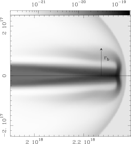
Figure 1: Density stratification of the region around the head of the jet obtained from model M1 for a $t=2000$ yr time-integration. The outer radius $r_{b}$ of the dense cocoon formed by the post-Mach disk jet material is indicated on the figure. The density is shown with a logarithmic greyscale, given by the bar on the top of the plot in g cm^-3. The two axes are labeled in cm, with the zero point corresponding to the centre of the initial jet cross section.

As an example of the results obtained from the computed jet models, in Figure 1 we show the density stratification of the jet head obtained from model M1 for a $t=2000$ yr integration time. From this Figure, we see that the dense, post-Mach disk jet material is ejected sideways, forming a cocoon which constitutes the “obstacle” which pushes the leading bow shock into the surrounding environment. Therefore, in order to compare the numerical simulations with the analytic model of §2, we associate the “radius of the obstacle” $r_{b}$ (see equation 4) with the cylindrical radius of the dense cocoon. We find that for the three computed models, the radius of the cocoon has oscillations of $\sim 20$% around a $r_{b}=10^{17}$ cm value. We therefore adopt this value in order to compare the X-ray luminosities predicted from the numerical simulations with the analytic model of §2.

Figure 2 shows the time-dependent X-ray luminosity of the heads of the jets computed from models M1, M2 and M3. The luminosities have been computed as follows. The frequency-dependent emission coefficient has been calculated using the Chianti data set and software (Dere et al. 2001), under the assumption of coronal ionization equilibrium and with solar abundances. This emission coefficient has then been integrated over energies ranging from 0.3 to 10 keV (in order to simulate Chandra observations), and over all of the volume of the computational domains of the jet models.

In Figure 2, we also show the values of $L_{x}$ obtained from our analytic model (see equations 7-9). For models M1 and M2, we obtain good agreement (within a factor of $\sim 2$) between the predictions from the numerical simulations and the analytic model.

For model M3, the $L_{x}$ values obtained from the numerical simulation range from a factor of $\sim 4$ to a factor of $\sim 10$ times the analytic prediction (see figure 2). This larger difference between the numerical and analytic predictions might be due to the fact that the cooling distance of model M3 is highly unresolved (see above).

We then conclude that the X-ray luminosities obtained from the numerical simulations and from the analytic model are in reasonably good agreement.

4 The X-ray luminosities of three bright HH objects

4.1 HH 2

This object has been marginally detected with Chandra by Pravdo et al. (2001), who estimated a (redenning corrected) X-ray luminosity of $L_{x}\approx{1.3\times 10^{-4}}L_{\odot}$. The detected emission is associated with the HH 2H condensation.

HST images of HH 2H (Schwartz et al. 1993) show that this condensation has a high intensity, elongated structure extending more or less perpendicular to the outflow axis. The lateral extension of this structure is of $\approx 2^{\prime\prime}.5$, which corresponds to a physical size of $\approx{1.7\times 10^{16}}$ cm (at a distance of 460 pc). We therefore have $r_{b}\approx{8.5\times 10^{15}}$ cm.

For the shock velocity and pre-shock density, we adopt the values estimated for HH 2H by Hartigan et al. (1987). Following these authors, we set $v_{bs}=150$ km s^-1 and $n_{0}=500$ cm^-3.

From equation (8) we then obtain $L_{x}={1.4\times 10^{-4}}L_{\odot}$. Therefore, the prediction obtained from our analytic model is in surprisingly good agreement with the HH 2H luminosity determined by Pravdo et al. (2001).

4.2 HH 154

HH 154 is a chain of aligned knots leading away from the L 1551 IRS 5 source. Favata et al. (2002) deduce that the X-ray emission that they detect comes from the high excitation knot D, for which they deduce (from previously published optical line ratios and line profiles) a $v_{bs}\approx 200$ km s^-1 bow shock velocity. Favata et al. (2002) and Fridlund & Lizeau (1994, 1998) deduce an $\approx 500$ cm^-3 density for the region upstream of knot D, and estimate that the density downstream of the knot has to be lower than this value by a factor of $\sim 15$ (taking the mean of the 10-20 range quoted by Fridlund & Lizeau 1998 for this factor). Therefore, we set $n_{0}\approx 100$ cm^-3. Finally, from the HST images of Fridlund & Lizeau (1998), we see that knot D has a diameter of $\approx 3^{\prime\prime}.3$, corresponding to $r_{b}={7.5\times 10^{15}}$ cm (at a distance of 150 pc).

With these parameters, from equation (8) we obtain $L_{x}={1.0\times 10^{-4}}L_{\odot}$. This luminosity is in uncannilly good agreement with the ${8\times 10^{-5}}L_{\odot}$ X-ray luminosity which Favata et al. (2002) deduced from their XMM-Newton observations.

4.3 HH 80/81

The HH objects with the highest excitation spectra are HH 80 and 81. These objects (discovered by Reipurth & Graham 1988) are associated with a thermal radio jet which shows proper motions of up to $\sim 1400$ km s^-1 (Martí et al. 1998).

HST images (Heathcote et al. 1998) show that HH 81 has an angular size of $\approx 3^{\prime\prime}.5$, corresponding to a physical size of $\approx{8.9\times 10^{16}}$ cm (at a distance of 1700 pc). We therefore adopt $r_{b}={4.5\times 10^{16}}$ cm. We also adopt the $v_{bs}\approx 700$ km s^-1 and $n_{0}\approx 400$ cm^-3 values deduced from the line widths and H$\alpha$ luminosity of HH 81 by Heathcote et al. (1988). Using these values, from equation (9) we obtain $L_{x}=0.46\,L_{\odot}$.

In order to estimate whether or not this object can be detected with Chandra, we have to calculate the energy flux $F_{HH~{}81}$ that would arrive at Earth. We use the distance of 1700 pc and the $A_{V}=2.33$ (corresponding to a $N_{H}\approx{3.0\times 10^{21}}$ cm^-2 neutral H column density) determined by Heathcote et al. (1998). If we consider the extinction at 1 keV, we obtain $F_{HH81}\approx{2.5\times 10^{-12}}$ erg s^-1 cm^-2, and if we use the extinction at 0.5 keV, we obtain $F_{HH81}\approx{7.5\times 10^{-15}}$ erg s^-1 cm^-2

Interestingly, the lower estimate that we have obtained for the flux that would be observed from HH 81 is an order of magnitude higher than the flux observed by Pravdo et al. (2001) for HH 2. Therefore, we conclude that HH 81 is a very good candidate for future Chandra observations.

5 Conclusions

We have derived a simple, analytic model for predicting the X-ray luminosity of HH bow shocks. We have tested this model against HH jet numerical simulations, showing that it is applicable for bow shocks with shock velocities in the $120\to 600$ km s^-1 range.

We have then applied the analytic model to obtain predictions of the X-ray luminosities of HH 2H, HH 154D and HH 81, and obtain the following results :

• the luminosity predicted for HH 2H is in good agreement with the Chandra observation of this object by Pravdo et al. (2001),

• the luminosity predicted for HH 154D is in good agreement with the XMM-Newton observation of this object by Favata et al. (2002),

• the X-ray luminosity predicted for HH 81 is a factor of $\sim 1000$ larger than the one of HH 2.

Because of the very large difference in X-ray luminosities predicted for HH 81 and for HH 2, even though HH 81 is a factor of $\sim 3$ more distant and more highly extinguished than HH 2, we expect it to be brighter than HH 2 by a factor of 10 to 100.

Figure 2: X-ray luminosity in the 0.3-10 keV energy range computed from models M1, M2 and M3 as a function of integration time. The horizontal lines represent the (time-independent) X-ray luminosity predicted for the appropriate parameters from the analytic model described in §2.