Early acceleration and adiabatic matter perturbations
in a class of dilatonic dark-energy models

Abstract

We estimate the growth of matter perturbations in a class of recently proposed dark-energy models based on the (loop-corrected) gravi-dilaton string effective action, and characterized by a global attractor epoch in which dark-matter and dark-energy density scale with the same effective equation of state. Unlike most dark-energy models, we find that the accelerated phase might start even at redshifts as high as $z\approx 5$ (thus relaxing the coincidence problem), while still producing at present an acceptable level of matter fluctuations. We also show that such an early acceleration is not in conflict with the recently discovered supernova SN1997ff at $z\approx 1.7$. The comparison of the predicted value of $\sigma_{8}$ with the observational data provides interesting constraints on the fundamental parameters of the given model of dilaton-dark matter interactions.

I Introduction

Independent cosmological observations have recently pointed out the existence of a significant fraction of critical density in the form of unclustered matter, possibly characterized by a negative pressure rie ; perl ; lee ; net . Such a component of the cosmic fluid, conventionally denoted dark energy, is believed to drive the accelerated evolution of our present Universe, as suggested by the study of the Supernovae Ia (SNIa) Hubble diagram. While the simplest explanation of the dark-energy component is probably a cosmological constant, it might be neither the most motivated, nor the best fit to the data.

The existence of a (presently dominating) dark-energy component raises at least three important questions: a) what is the physical origin of such a new component? b) why its energy density today is just comparable to the matter energy density? c) did the acceleration start only very recently in the cosmological history?

The first question refers to the fundamental physical mechanism able to generate a cosmic and universal dark-energy distribution. So far, most models of dark energy have adopted a purely phenomenological approach, even if a few proposal concerning the possible role of the dark-energy field in the context of fundamental physics have already appeared fri ; wet90 ; albre ; MG01 ; GPV01 ; pie .

The other questions concern two distinct (although possibly related) aspects of the so-called “coincidence problem” Ste . The first aspect refers to the density of the dark-energy and of the dark-matter component. Since in most models the two components have different equations of state, they scale with time in a different way, and their densities should be widely different for essentially all the cosmological history: by contrast, current data are strongly pointing at a comparable proportion of the two components just at the present epoch.

The second aspect of the coincidence problem may arise if the epoch of accelerated evolution started only very recently, say at $z\approx 1$. There are reasons to suspect that this may be the case because, in most models, the growth of structures is forbidden after the beginning of the accelerated expansion, so that the acceleration cannot be extended too far into the past. It has also been recently claimed that the supernova SN1997ff super ; super1 at $z\approx 1.7$ provides an additional indication that the acceleration is a relatively recent phenomenon.

A promising approach for a possible simultaneous answer to the above questions has been recently provided by a dilatonic interpretation of the dark energy based on the infinite bare-coupling limit of the superstring effective action GPV01 , whose cosmological solutions are characterized by a late-time global attractor where dark-matter and (dilatonic) dark-energy densities have an identical scaling with time. A very similar cosmological scenario has been studied also in amtoc ; bias . The respective amount of dark-matter and dark-energy density is eventually determined by the fundamental constants of the model, and it is expected to be of the same order, so that their ratio keeps frozen around unity for the whole duration of such an asymptotic regime. In such a context, the today approximate equality of dark-matter and dark-energy density would be no longer a coincidence of the present epoch, but a consequence of the fact that our Universe has already entered the asymptotic regime (actually, for a region of parameter space allowed by observations, it is also possible that the ratio of dark-energy to dark-matter density is close to unity not only in the asymptotic regime, but already after the equivalence epoch). Finally, the cosmic field responsible for the observed large-scale acceleration would be no longer introduced ad hoc, being identified with a fundamental ingredient of superstring/M-theory models of high-energy physics.

In this paper we will focus our discussion on the possible constraints imposed by structure formation on the above model of dilatonic dark energy, by studying the growth of matter perturbations in the two relevant post-equivalence epochs: a first decelerated epoch, dubbed dragging phase, and a second accelerated epoch, dubbed freezing phase. We will then reconstruct the behavior of the cosmological gravitational potential, evaluate the Sachs-Wolfe and integrated Sachs-Wolfe contributions to the spectrum of CMB anisotropies, and estimate the present level of matter fluctuations (in particular, the so-called variance $\sigma_{8}$, smoothed out over spheres of radius 8 Mpc $h^{-1}$). Finally, we will compare it with observations.

The results that we find are interesting, and might help answering the third question posed at the beginning of this section: among the range of parameters compatible with a phenomenologically acceptable $\sigma_{8}$ we find indeed values allowing a long epoch of acceleration, starting as far in the past as at $z\approx 5$. By contrast, the models of dark energy uncoupled to dark matter, with frozen (or slowly varying) equation of state, cannot accelerate before $z\approx 1$ . It seems appropriate to anticipate here that the production of an acceptable level of fluctuations even in the case of an early start of the accelerated epoch is due to two concurrent factors: the first is that, during the freezing phase, perturbations do not stop growing like in other models of accelerating dark energy; the second is that the horizon at equivalence in our model shifts at larger scales with respect to a standard $\Lambda$CDM model. It is also important to stress that such an early acceleration is by no means in contrast with the recently observed supernova SN1997ff at $z\approx 1.7$.

For the model of dilatonic dark energy considered in this paper the coincidence problem can thus be alleviated by the fact that the ratio of dark-matter to dark-energy density is of order one not only at present, not only in the course of the future evolution but (at least in principle) also in the past, long before the present epoch. It should be clear, however, that this possibility could be strongly constrained by future observations of supernovae at high redshift.

The paper is organized as follows. In Sect. II we present the details of our late-time, dilaton-driven cosmological scenario, and define the (theoretical and phenomenological) parameters relevant to our computation. In Sect. III we discuss the growth of matter perturbations and compute the variance $\sigma_{8}$. In Sect. IV we impose the observational constraints on our set of parameters, and determine the maximal possible extension towards the past of the phase of accelerated evolution. We also find, as a byproduct of our analysis, interesting experimental constraints on the fundamental parameters of the string effective action used for a dilatonic interpretation of the dark-energy field. In Sect. V we compare our model with the constraints provided by the farthest observed supernova at $z\approx 1.7$. Our conclusions are finally summarized in Sect. VI.

II The model

The model we consider is based on the gravi-dilaton string effective action GSW87 which, to lowest order in the higher-derivative expansion, but including dilaton-dependent loop corrections and a non-perturbative potential, can be written in the String-frame as follows GPV01

$$S=-{1\over 2\lambda_{s}^{2}}\int d^{4}x\sqrt{-\widetilde{g}}\left[e^{-\psi(\phi)}\widetilde{R}+Z(\phi)\left(\widetilde{\nabla}\phi\right)^{2}+{2\lambda_{s}^{2}}\widetilde{V}(\phi)\right]+S_{m}(\widetilde{g},\phi,{{\textrm{matter}).}}$$ (1)

Here $\lambda_{s}$ is the fundamental string-length parameter, and the tilde refers to the String-frame metric. The functions $\psi(\phi),Z(\phi)$ are appropriate “form factors" encoding the dilatonic loop corrections and reducing, in the weak coupling limit, to the well known tree-level expressions GSW87 $Z=\exp(-\psi)=\exp(-\phi)$.

In this paper we are interested in a “late-time", post-big bang cosmological scenario, in which the dilaton is free to run to infinity rolling down an exponentially suppressed potential, and the loop form factors approach a finite limit as $\phi\rightarrow+\infty$. Assuming the validity of an asymptotic Taylor expansion Ven01 , and following the spirit of “induced-gravity" models in which the gravitational and gauge couplings saturate at small values because of the large number ($N\sim 10^{2}$) of fundamental GUT gauge bosons entering the loop corrections, we can write, for $\phi\rightarrow+\infty$,

$$e^{-\psi(\phi)}\,=\,c_{1}^{2}+b_{1}e^{-\phi}+{{\mathcal{O}}}(e^{-2\phi}),\;Z(\phi)\,=\,-c_{2}^{2}+b_{2}e^{-\phi}+{{\mathcal{O}}}(e^{-2\phi})\;,$$

$$\widetilde{V}(\phi)\,=\,V_{0}\,e^{-\phi}+{{\mathcal{O}}}(e^{-2\phi}).$$ (2)

The dimensionless coefficients $c_{1}^{2},c_{2}^{2}$ are typically of order $10^{2}$, because of their quantum-loop origin. We may note, in particular, that $c_{1}^{2}$ asymptotically controls the fundamental ratio between the (dimensionally reduced) string and Planck scales GPV01 , $c_{1}^{2}=\lambda_{s}^{2}/\lambda_{P}^{2}$, which is indeed expected to be in the range Kap85 $\lambda_{P}/\lambda_{s}\simeq 0.3-0.03$.

To complete the model we have to specify the matter action $S_{m}$ of eq. (1), containing the coupling (possibly renormalized by loop corrections) of the matter fields to the dilaton. The variation of $S_{m}$ with respect to $\phi$ defines the (String-frame) dilatonic charge density $\widetilde{\sigma}$, whose appearance is a peculiar string theory effect Gas99 , and represents the crucial difference from conventional (Brans-Dicke) scalar-tensor models of gravity.

For the cosmological scenario of this paper we shall assume, as in GPV01 , that $S_{m}$ contains radiation, baryons and cold dark matter, and that the dilatonic charge of the dark matter component switches on at sufficiently large couplings, being proportional (through a time-dependent factor $q(\phi)$) to its energy density $\widetilde{\rho}{{}_{c}}$. Also, $q(\phi)$ is assumed to approach a constant (positive) value $q_{0}$ as $\phi\rightarrow+\infty$,

$$q(\phi)=q_{0}+{{\mathcal{O}}}(e^{-q_{0}\phi}).$$ (3)

The dilatonic charge of radiation and of ordinary baryonic matter are instead exponentially suppressed in the strong coupling regime GPV01 , and this guarantees the absence of unacceptably large corrections to macroscopic gravity, since in the model we are considering the dilaton is asymptotically massless and leads to long-range scalar interactions (see however DPV02 for possible testable violations of the equivalence principle, and other non-standard effects, possibly observable in such a context).

By considering an isotropic, spatially flat metric background, and a perfect fluid model of matter sources, it is now convenient to write the cosmological equations for the action (1) directly in the Einstein frame, defined by the conformal transformation $\widetilde{g}_{\mu\nu}=c_{1}^{2}g_{\mu\nu}\exp(\psi)$. In the cosmic-time gauge (and in units $2\lambda_{P}^{2}\equiv 16\pi G=1$) the equations are GPV01

$$6H^{2}=\rho{+}\rho{{}_{\phi}},\quad 4\dot{H}+6H^{2}=-p-p_{\phi},$$ (4)

$$k^{2}(\phi)\left(\ddot{\phi}+3H\dot{\phi}\right)+k(\phi)\,k^{\prime}(\phi)\,\dot{\phi}^{2}+{V}^{\prime}(\phi)+\frac{1}{2}\left[{\psi^{\prime}(\phi)}(\rho_{b}+\rho{{}_{c}})+q(\phi)\rho{{}_{c}}\right]=0,$$ (5)

where a prime denotes differentiation with respect to $\phi$, and

$$k^{2}(\phi)=3\psi^{\prime 2}-2e^{2\psi}Z, \quad V=c_{1}^{4}e^{2\psi}\widetilde{V},\quad q(\phi)={\sigma_{c}/\rho{{}_{c}}},$$ (6)

$$\rho{{}_{\phi}}={1\over 2}k^{2}(\phi)\dot{\phi}^{2}+V(\phi), p_{\phi}={1\over 2}k^{2}(\phi)\dot{\phi}^{2}-V(\phi),$$ (7)

$$\rho{=}\rho{{}_{r}}+\rho{{}_{b}}+\rho{{}_{c}}, p=\rho{{}_{r}}/3.$$ (8)

We have explicitly separated the radiation, baryon and cold dark matter components ($\rho{{}_{r}},\rho{{}_{b}},\rho{{}_{c}}$), and introduced the (Einstein-frame) dilatonic charge per unit of gravitational mass, $q(\phi)$, which is non-vanishing (at large enough $\phi$) only for the dark-matter component. The combination of the above equations leads to the separate energy conservation equations:

$$\dot{\rho}{{}_{r}}+4H\rho{{}_{r}}=0,$$ (9)

$$\dot{\rho}{{}_{b}}+3H\rho{{}_{b}}-{1\over 2}\dot{\phi}{\psi^{\prime}}\rho{{}_{b}}=0,$$ (10)

$$\dot{\rho}{{}_{c}}+3H\rho{{}_{c}}-{1\over 2}\dot{\phi}\left({\psi^{\prime}}+q\right)\rho{{}_{c}}=0,$$ (11)

$$\dot{\rho}{{}_{\phi}}+3H(\rho{{}_{\phi}}+p_{\phi})+{1\over 2}\dot{\phi}\left[{\psi^{\prime}}(\rho_{b}+\rho{{}_{c}})+q\rho{{}_{c}}\right]=0.$$ (12)

With the above assumptions on $\psi,Z$ and $q$, and for appropriate values of the parameters of the loop functions (in particular, for a sufficiently small value of $V_{0}$), it has been shown in GPV01 that the phase of standard, matter-dominated evolution is modified by the non-minimal, direct coupling of dark matter and dilatonic dark energy. After the equivalence epoch, in particular, the Universe may enter a phase of “dragging", followed by an accelerated phase of asymptotic “freezing". For the reader’s convenience we recall here the main properties of such two phases, referring to GPV01 ; amtoc for a more detailed discussion (see also ame3 for a general study of the dynamical system).

(1) “Dragging" phase. The potential $V(\phi)$ is negligible, the evolution is decelerated, $\rho{{}_{\phi}}$ is still subdominant (as well as $\rho{{}_{b}}$), but $\rho{{}_{\phi}}$ evolves in time like the dominant component $\rho{{}_{c}}$, so that the dilaton dark energy is “dragged" along by the dark matter density.

In this phase $k(\phi)$ can be approximated by a constant, $k(\phi)=k_{1}$, and it is thus convenient to define the rescaled field $\widehat{\phi}=k_{1}\phi$ which has canonical kinetic term in the action, and which satisfies with $\rho{{}_{c}}$ the system of coupled equations

$${\ddot{\widehat{\phi}}}+3H{\dot{\widehat{\phi}}}+{1\over 2}\left(\psi^{\prime}+q\over k\right)\rho{{}_{c}}=0,$$ (13)

$$\dot{\rho}{{}_{c}}+3H\rho{{}_{c}}-{1\over 2}\left(\psi^{\prime}+q\over k\right)\rho{{}_{c}}{\dot{\widehat{\phi}}}=0,$$ (14)

We can then define the canonical effective coupling of the dilaton to dark matter by the function $\beta(\phi)$, defined by:

$$\frac{1}{\sqrt{3}}\beta(\phi)={1\over 2}{\psi^{\prime}(\phi)+q(\phi)\over k(\phi)}$$ (15)

which, in the dragging phase, is also approximated by a constant, $\beta(\phi)=\beta_{1}\ll 1$ (the conventional factor $1/\sqrt{3}$ has been introduced here to adapt the notations of this paper to previous studies of the dark-matter-scalar system ame3 ).

Using eqs. (4), (13) we find, in the dragging phase GPV01 ,

$${\dot{\widehat{\phi}}}=-4H\beta_{1}/\sqrt{3},$$ (16)

so that, from eq. (14),

$$\rho{{}_{c}}\sim H^{2}\sim\rho{{}_{\phi}}\sim a^{-(3+4\beta_{1}^{2}/3)}.$$ (17)

Because of the dragging the time evolution of the dark matter density deviates from the typical behaviour of dust sources, in such a way that $\rho{{}_{c}}$ decays slightly faster than energy density of baryons, $\rho{{}_{b}}\sim a^{-3}$. It is however unlikely that this effect may lead the Universe to a baryon-dominated phase, because this trend is soon inverted in the subsequent, freezing phase.

(2) “Freezing" phase. The asymptotic dilaton potential $V(\phi)=V_{0}\exp(-\phi)$ comes into play, the evolution (for large enough values of $q$) is accelerated, the dark matter, potential and (dilatonic) kinetic energy densities evolve in the same way, so that the ratio $\rho{{}_{\phi}}/\rho{{}_{c}}$ is frozen to an arbitrary constant value. The critical fraction of dark matter, potential and kinetic energy densities are also separately constant throughout this phase GPV01 ; ame3 .

In such a phase, asymptotically approached when $\phi\rightarrow+\infty$, one has $q(\phi)=q_{0}$, $\psi^{\prime}=0$, and the parameters $k(\phi),\beta(\phi)$ can be again approximated by constant values $k_{2},\beta_{2}$ (in general different from the previous ones), related by $k_{2}\beta_{2}=\sqrt{3}q_{0}/2$. The coupled equations for the canonically rescaled field $\widehat{\phi}=k_{2}\phi$ are modified by the presence of the potential

$${\ddot{\widehat{\phi}}}+3H{\dot{\widehat{\phi}}}+{\partial V\over\partial\widehat{\phi}}+\frac{\beta_{2}}{\sqrt{3}}\rho{{}_{c}}=0,$$ (18)

$$\dot{\rho}{{}_{c}}+3H\rho{{}_{c}}-\frac{\beta_{2}}{\sqrt{3}}\rho{{}_{c}}{\dot{\widehat{\phi}}}=0,$$ (19)

and, together with eq. (4), are solved by the following configuration GPV01 :

$$V=V_{0}e^{-\widehat{\phi}/k_{2}}\sim({\dot{\widehat{\phi}}})^{2}\sim\rho{{}_{\phi}}\sim\rho{{}_{c}}\sim H^{2}\sim a^{-6/(2+q_{0})}.$$ (20)

In units of critical energy density we find, in particular,

$$\Omega_{V}={V\over 6H^{2}}=\Omega_{k}+{q_{0}\over 2+q_{0}}, \Omega_{k}={({\dot{\widehat{\phi}}})^{2}\over 12H^{2}}={3k_{2}^{2}\over(2+q_{0})^{2}},$$

$$\Omega_{\phi}=\Omega_{V}+\Omega_{k}, \Omega_{c}=1-\Omega_{\phi}.$$ (21)

Note that, from eq. (20),

$${\ddot{a}\over aH^{2}}=1+{\dot{H}\over H^{2}}={q_{0}-1\over q_{0}+2},$$ (22)

so that the freezing phase is accelerated for $q_{0}>1$. In that case, according to eq. (20), the dark matter density tends to be strongly enhanced (as time goes on) with respect to the baryon density, which on the contrary is uncoupled to the dilaton and thus evolves in the standard way, $\rho{{}_{b}}\sim a^{-3}$. As already pointed out in GPV01 ; AT01a , it is tempting to speculate, in such a context, that the present smallness of the ratio $\rho{{}_{b}}/\rho{{}_{c}}$ could then emerge as an artifact of a long enough freezing phase, started before the present epoch.

In this paper, in order to discuss the possible bounds imposed by present observations on the above scenario, we will consider a simplified model of late-time (i.e., after-equivalence) cosmology, consisting of two phases. More precisely, we will drastically approximate the background evolution by assuming that the Universe performs a sudden transition from the radiation-dominated to the dragging phase at the equivalence epoch $a=a_{{\textrm{eq}}}$, and from the dragging to the freezing phase at the transition epoch $a=a_{f}$. We will discuss in this context the phenomenological constraints on the parameters of the string effective action, and in particular their possible consistency with an early beginning of the freezing epoch, $z_{f}=(a_{0}/a_{f})-1\gg 1$, which (as already mentioned) may be relevant for a truly satisfactory solution of the coincidence problem.

To make contact with previous results we will use here the following explicit model of dilaton potential, charge and loop corrections (already adopted in GPV01 ):

$$e^{-\psi(\phi)}\,=\,e^{-\phi}+c_{1}^{2},\quad Z(\phi)\,=\,e^{-\phi}-c_{2}^{2},\quad q(\phi)\,=q_{0}\,{e^{q_{0}\phi}\over c^{2}+e^{q_{0}\phi}},$$ (23)

$$V(\phi)\,\,=c_{1}^{4}\,\,m_{V}^{\,2}e^{2\psi}\left[\exp\,(-e^{-\phi}/\alpha_{1})-\exp\,(-e^{-\phi}/\alpha_{2})\right],\quad 0<\alpha_{2}<\alpha_{1}.$$ (24)

Here $c_{1}^{2},c_{2}^{2},c^{2}$ are numbers of order $10^{2}$, the asymptotic charge satisfies $q_{0}>1$ to guarantee a final accelerated regime, and the dilaton potential reduces asymptotically to the exponential form of eq. (2), with $V_{0}=m_{V}^{2}(\alpha_{1}-\alpha_{2})/\alpha_{1}\alpha_{2}$ (in units $2\lambda_{P}^{2}=1$). It is worth noting that the mass scale $m_{V}$, controlling asymptotically the amplitude of the potential (and thus the beginning of the freezing phase), is possibly expected to be of non-perturbative origin, and thus related to the fundamental string scale in a typical instantonic way,

$$m_{V}=\exp\left[-{2\over\beta^{*}{\alpha}_{{\textrm{GUT}}}}\right]M_{s},$$ (25)

where $\alpha_{{\textrm{GUT}}}\simeq 1/25$ is the asymptotic value of the GUT gauge coupling, and $\beta^{*}{}$ is some model-dependent loop coefficient. As noted in GPV01 , a value of $\beta^{*}$ slightly smaller than the usual coefficient of the QCD beta-function is already enough to move $m_{V}$ from the QCD scale down to the scale relevant for a realistic scenario of dark-energy domination; a typical reference value is, for instance, $\beta^{*}\simeq 0.36$, which corresponds to $m_{V}\sim H_{0}\sim 10^{-61}M_{P}$, and thus to a freezing phase starting around the present epoch.

With the above explicit forms of the loop corrections we can now compute the constant parameters for the dragging ($k_{1},\beta_{1}$) and the freezing ($k_{2},\beta_{2}$) eras. By setting $\mu_{2}=\sqrt{3}c_{1}/(\sqrt{2}c_{2})$ we find

$$k_{1}={\sqrt{3}\over\mu_{2}},\quad\beta_{1}={q_{0}\mu_{2}\over 2c^{2}},\quad k_{2}={\sqrt{3}\over\mu_{2}},\quad\beta_{2}={q_{0}\mu_{2}\over 2}.$$ (26)

The constant $\mu_{2}/\sqrt{3}$ represents the slope of the dilaton potential $V(\widehat{\phi})$ during freezing. With these definitions, $q_{0}=2\beta{{}_{2}}/\mu_{2},c^{2}=\beta{{}_{2}}/\beta{{}_{1}}$.

For our model of background we can finally express the phenomenological variables, required for the subsequent computations, in terms of the above set of parameters. From eqs. (17), (20) we get the barotropic parameter $w=(p_{tot}/\rho_{tot}{)}+1$ relative to the effective equation of state of cold dark matter,

$$w_{1}=1+{4\over 9}\beta_{1}^{2},\quad w_{2}={2\over 2+q_{0}}={\mu_{2}\over\mu_{2}+\beta{{}_{2}}},$$ (27)

in the dragging and freezing eras, respectively. Another useful parameter is $\Omega_{c}$: in the dragging phase, from eq. (16),

$$\Omega_{c}=1-\Omega_{\phi}=1-{({\dot{\widehat{\phi}}})^{2}\over 12H^{2}}=1-{4\over 9}\beta{{}_{1}}^{2}.$$ (28)

In the freezing phase, from eq. (21),

$$\Omega_{c}={2\mu_{2}^{2}+2\beta{{}_{2}}\mu_{2}-9\over 2(\beta{{}_{2}}+\mu_{2})^{2}}.$$ (29)

(this is therefore to be identified to the value observed today).

Note that the ratio of dark-energy to dark-matter density may be close to unity throughout the cosmic evolution after equivalence, if the constants $\beta_{1},\beta_{2},\mu_{2}$ are of the order of unity. In this sense, in such a model, it is even possible that a serious coincidence problem never really arises. By contrast, dark-energy models without a stationary phase in which $\rho{{}_{m}}\sim\rho{{}_{\phi}}$ (see e.g. cald ; kessence ) have to explain the today value (or order one) of ratios $\Omega_{\phi}/\Omega_{m}$ which range from extremely small values in the past to unboundedly large values in the future amtoc .

We end this section with the computation of three useful red-shift parameters $z_{e},z_{f},z_{b}$ corresponding, respectively, to the radiation-matter equivalence, to the beginning of the freezing epoch, and to the baryon epoch (associated to a possible baryon-dominated phase). From the behaviour of $\rho{{}_{\phi}}$ and $\rho{{}_{b}}$ in the freezing phase,

$$\rho{{}_{\phi}}=\rho{{}_{\phi}}(a_{0})\left(a_{0}\over a\right)^{3w_{2}},\quad\rho{{}_{b}}=\rho{{}_{b}}(a_{0})\left(a_{0}\over a\right)^{3},$$ (30)

we can determine the baryon red-shift epoch $a_{b}$, such that $\rho{{}_{\phi}}=\rho{{}_{b}}$, as follows AT01a :

$$1+z_{b}={a_{0}\over a_{b}}=\left(\Omega_{\phi}\over\Omega_{b}\right)_{0}^{\mu_{2}+\beta{{}_{2}}\over 3\beta{{}_{2}}}.$$ (31)

The present ratio $(\Omega_{\phi}/\Omega_{b})_{0}$ is a known observational input. Our model excludes the possibility of a baryon-dominated phase and thus requires, for consistency, $z_{b}>z_{f}$ (see AT01a for a dark-energy model with a baryonic epoch).

The equivalence scale can be obtained by rescaling $\rho{{}_{c}}$ and $\rho{{}_{r}}$ from $a_{e}$ down to $a_{0}$, i.e.

$$\rho{{}_{c}}(a_{0})=\rho{{}_{c}}(a_{e})\left(a_{e}\over a_{f}\right)^{3w_{1}}\left(a_{f}\over a_{0}\right)^{3w_{2}},\quad\rho{{}_{r}}(a_{0})=\rho{{}_{r}}(a_{e})\left(a_{e}\over a_{f}\right)^{4}\left(a_{f}\over a_{0}\right)^{4},$$ (32)

from which

$$1+z_{e}={a_{0}\over a_{e}}=\left[\left(\Omega_{r}\over\Omega_{c}\right)_{0}\left(a_{f}\over a_{0}\right)^{3(w_{2}-w_{1})}\right]^{1\over 3w_{1}-4},$$ (33)

where, again, $(\Omega_{r}/\Omega_{c})_{0}$ is an observational input. Similarly, we can determine the freezing epoch by rescaling the dilaton potential energy,

$$\rho{{}_{V}}(a_{f})=V_{0}e^{-\phi_{f}}=\rho{{}_{V}}(a_{0})\left(a_{0}\over a_{f}\right)^{3w_{2}}.$$ (34)

Here $\rho{{}_{V}}(a_{0})=6H_{0}^{2}\Omega_{V}$, where $\Omega_{V}$ is determined by eq. (21), and $\phi_{f}$ is the transition scale between small and large values of the dilaton charge, namely $\phi_{f}=(2/q_{0})\ln c$, from eq. (23). We thus obtain

$$1+z_{f}={a_{0}\over a_{f}} = \left[{V_{0}\over 6H_{0}^{2}\Omega_{V}}\left(\beta{{}_{1}}\over\beta{{}_{2}}\right)^{\mu_{2}\over 2\beta{{}_{2}}}\right]^{\mu_{2}+\beta{{}_{2}}\over 3\mu_{2}},$$ (35)

$$\Omega_{V} = {9+4\beta{{}_{2}}(\mu_{2}+\beta{{}_{2}})\over 4(\mu_{2}+\beta{{}_{2}})^{2}},$$ (36)

where $H_{0}$ is the value of the Hubble parameter provided by present observations.

In conclusion, we have a four-parameter model of background, spanned by two possible (related) sets of independent variables: the phenomenological variables $\{\beta{{}_{1}},\beta{{}_{2}},\mu_{2},z_{f}\}$ or, equivalently, the fundamental variables $\{c_{1}/c_{2},c^{2},q_{0},V_{0}\}$, referred to the $\phi\rightarrow+\infty$ limit of the string effective action of eq. (1). The mapping between the two sets is defined by eqs. (26) and (36). Note that two of the four parameters can be in principle determined by fitting the observational data relative to the present fraction of cold dark matter, $\Omega_{c}$, and the dark-energy equation of state, $w_{2}$: we can determine, for instance, $\mu_{2}$ and $\beta{{}_{2}}$ through eqs. (26), (29). In the following sections we will discuss the allowed regions left by various phenomenological constraints in such a parameter space.

III Constraints from structure formation

In this Section we will compute the r.m.s. dark-matter density contrast $\sigma_{8}$ for the model presented in Sect. II, combining it with the CMB angular power spectrum (at low multipoles) in order to eliminate the dependence on the normalization factor. Another analytical computation of $\sigma_{8}$ including dark energy has recently been presented in doran e schwindt , but only for models in which dark energy and dark matter are uncoupled.

Before starting the computation, let us recall some preliminary condition to be imposed (for consistency) on our model of background.

III.1 Consistency conditions on the background

As illustrated in Sect. II, the evolution of our cosmological background is characterized by two stationary ($\rho_{c}\sim\rho_{\phi}$) stages: the dragging era (labelled by the subscript $1$), and the final accelerated freezing era (labelled by $2$). This scenario can be consistently implemented provided the parameters are chosen in such a way as to satisfy the following conditions.

First, the dragging era exists, and is a saddle point of our dynamical system, only if ame3 :

$$\left|\beta_{1}\right|<{\sqrt{3}}/{2}\simeq 0.87.$$ (37)

Second, in order for the baryons not to dominate (in the past) over the dark-matter component, it is necessary to impose (as anticipated):

$$z_{b}>z_{f}.$$ (38)

Third, the final freezing phase is accelerated only if:

$$\mu_{2}<2\beta_{2}.$$ (39)

The current SNIa observations, however, require more than simply an acceleration, as shown by a recent analysis Dalal of SNIa data in models which include a freezing epoch. The result is that only models with an effective equation of state $w_{2}\approx 0.4$ (best fit) or $w_{2}<0.5$ (at one sigma) are consistent with the SNIa Hubble diagram.

In the following discussion we will reduce, for simplicity, our set of free parameters by using the observed CDM fraction of critical density, $\Omega_{c}\simeq 0.3$, as a fixed observational input. This can be used to eliminate $\mu_{2}$ through eq. (29), in such a way that we are left with three parameters only, $\beta{{}_{1}},\beta{{}_{2}}$ and $z_{f}$. In that case, the above limits on $w_{2}=\mu_{2}/(\mu_{2}+\beta_{2})$ define two reference values for $\beta_{2}$,

$$\beta_{2} = 4.02,\>{(\textrm{best fit })}$$ (40)

$$\beta_{2} = 2.35,\>{(\textrm{one sigma })},$$ (41)

which will be used in our subsequent analysis. For future reference, note that the lower limit at 95% c.l. is $\beta_{2}>1.55$. We note, finally, that pushing back in time the transition between the dragging and freezing eras, that is increasing $z_{f},$ implies a decrease of $z_{e}$. The condition

$$z_{f}\leavevmode\nobreak\ \raise 1.54996pt\hbox{$<$}\kern-7.20003pt\lower 2.40247pt\hbox{$\sim$}\leavevmode\nobreak\ 100$$ (42)

prevents the unwanted crossing of these two quantities.

All the above constraints will be imposed on our subsequent computations.

III.2 Angular power spectrum at low multipoles

In this subsection we will extend the treatment of the Sachs-Wolfe effect presented in HuW (to which we refer for the notation) in such a way as to include the case of coupled dark energy and dark matter. We shall assume a conformally flat metric, $ds^{2}=a^{2}(d\tau^{2}-dx^{i}dx_{i})$, and we shall exploit the fact that, in the absence of anisotropic stress, the two scalar potentials $\Psi$ and $\Phi$ defined in the longitudinal gauge turn out to be equal and to coincide, in the Newtonian limit, with the usual gravitational potential. The general expressions for the Sachs-Wolfe (SW) and integrated Sachs-Wolfe (ISW) parts of the angular power spectrum, for adiabatic scalar perturbations, can then be written as HuW :

$$C_{\ell}^{SW} = \frac{2}{9\pi}\int dkk^{2}\left|\Psi(k,\tau_{d})\right|^{2}j_{\ell}^{2}[k(\tau_{0}-\tau_{d})],$$ (43)

$$C_{\ell}^{ISW} = 2G^{2}_{2}(\ell)\int dk\left|{\Psi}^{\prime}(k,\tau_{\ell})\right|^{2},$$ (44)

where $G_{2}(\ell)={\Gamma[(\ell+1)/2]}/{\Gamma[(\ell+2)/2]}$, $j_{\ell}$ are the spherical Bessel functions, the prime denotes differentiation with respect to conformal time, and $\tau_{d}$ is the conformal time at decoupling, while $\tau_{\ell}=\tau_{0}-(\ell+1/2)/k$ (notice that the above expression for the ISW coefficient has been already integrated over $\tau$).

Let us denote with $\delta_{k}$ the CDM density contrast for the wavemode $k$, and with $\widehat{\phi}$ and $\chi\equiv\delta\widehat{\phi}$, respectively, the values of the background scalar field and of its fluctuation. The label $0$ will denote the present time $t_{0}$, and it is to be understood that all the density parameters $\Omega_{c},\Omega_{b}$, etc. are always referred to the present time, unless otherwise stated. Finally, all perturbation variables will be expressed in terms of their Fourier components. The potential $\Psi$ is then determined by the relativistic Poisson equation (in units $16\pi G=1$)

$$\Psi(a)=-\frac{3}{2k^{2}}H_{0}^{2}\Omega_{c}\delta_{k}(a_{0})s(k,a)-\frac{1}{4k^{2}}{\chi}^{\prime}{\widehat{\phi}}^{\prime}-\frac{3aH}{4k^{2}}\chi{\widehat{\phi}}^{\prime}-\frac{a^{2}}{4k^{2}}{\chi}\frac{dV}{d{\widehat{\phi}}},$$ (45)

where we have introduced the (possibly $k$-dependent) function $s(k,a)$, which accounts for the time-evolution of the dark matter and of its density contrast, according to the equations

$$\rho_{c}(a) = \rho_{c}(a_{0})f(a),$$ (46)

$$\delta_{k}(a) = \delta_{k}(a_{0})D(k,a),$$ (47)

$$s(k,a) = D(k,a)f(a)\left(\frac{a}{a_{0}}\right)^{2}.$$ (48)

The quantities appearing in the r.h.s. of eq. (45) are evaluated in the synchronous gauge, while the potential $\Psi$ is calculated in the longitudinal gauge HuW , since this helps extending the validity of the Poisson equation to all scales. Note that we have dropped from the Poisson equation the contribution of the dark-matter velocity fluctuations, since it can be shown that they are negligible bias . The baryon contribution has been neglected as well. Defining the matter power spectrum $P(k)=|\delta_{k}(a_{0})|^{2}$, it follows that

$$C_{\ell}^{SW} = \frac{1}{2\pi}H_{0}^{4}\Omega_{c}^{2}(1+\Sigma)\int\frac{dk}{k^{2}}P(k)|s(k,a_{d})|^{2}j_{\ell}^{2}[k(\tau_{0}-\tau_{d})],$$ (49)

$$C_{\ell}^{ISW} = \frac{9}{2}H_{0}^{4}\Omega_{c}^{2}G^{2}_{2}(\ell)(1+\Pi)\int\frac{dk}{k^{4}}P(k)\left|s^{\prime}[k,a(\tau_{\ell})]\right|^{2}.$$ (50)

The functions $\Sigma$ and $\Pi$ represent corrections due to the scalar field contribution. In the next few paragraphs we will neglect these effects, concentrating the attention only on the dark-matter part of the power spectrum, while the scalar contribution will be reconsidered at the end of our calculation. The convenience of this procedure will become apparent later on.

Focusing our attention on the background evolution after the epoch of matter-radiation equivalence, we can now specify the evolution of the CMB energy density by setting

$$f(a) = (a/a_{0})^{-3w_{2}},\qquad a>a_{f}$$ (51)

$$= (a_{f}/a_{0})^{-3w_{2}}(a/a_{f})^{-3w_{1}},\qquad a<a_{f}.$$ (52)

where $w_{1,2}$ were defined in eqs. (27). For what concerns the growth of matter perturbations, since we are interested in the low-multipole branch of the spectrum, it is reasonable to consider only scales that reenter the horizon after equivalence (and before freezing, as in the accelerated stage no reenter is possible). The growth of $\delta_{k}$ has been derived in bias as a function of the parameters $\beta{}$ and $\mu$ of the dragging and freezing epochs. It turns out that the evolution is the same for all modes:

$$D(k,a) = (a/a_{0})^{m_{2}},\quad a>a_{f}$$

$$= (a/a_{f})^{m_{1}}(a_{f}/a_{0})^{m_{2}},\quad a<a_{f},$$

where

$$m_{1}=1+\frac{4}{3}\beta^{2}_{1},\quad m_{2}={\Delta-10\beta_{2}-\mu_{2}\over 4\left(\beta_{2}+\mu_{2}\right)},$$ (53)

and

$$\Delta^{2}=-108+44\beta_{2}\mu_{2}+32\beta^{3}_{2}\mu_{2}+25\mu^{2}_{2}+\beta^{2}_{2}\left(32\mu^{2}_{2}-44\right)$$ (54)

(in the dragging phase the same exponent $m_{1}$ describes the growth of perturbations both inside and outside the horizon). Considering scales with $k<k_{d}$, where the subscript $d$ stands for decoupling, the relevant function for the computation of the ordinary SW effect can thus be parametrized by a $k$-independent function as follows:

$$s(a_{f})=(a_{d}/a_{f})^{m_{1}-3w_{1}}(a_{f}/a_{0})^{m_{2}-3w_{2}}(a_{d}/a_{0})^{2}=(a_{f}/a_{0})^{\alpha_{2}}.$$ (55)

where $\alpha_{2}\equiv m_{2}-3w_{2}+2$ (note that $\alpha_{1}\equiv m_{1}-3w_{1}+2=0$).

Some comments are now in order, concerning the evolution of perturbations described by the above equations. First we notice that in the dragging phase $m_{1}>1$, i.e. that the perturbations growth is faster than in a standard CDM model. This is due to an extra pull on dark matter arising from the dark-energy coupling, that act as an additional (scalar) gravity force bias . Secondly, the growth in the accelerated freezing regime does not vanish asymptotically, like in other dark-energy models. This is again an effect of the dark energy-dark matter coupling and of the fact that the dark-matter density is not driven to zero by the acceleration. Finally, since the baryons are decoupled from the dilaton, they evolve differently, and a bias between the baryons and the dark-matter distribution is expected. The constraints from this effect have been discussed in ref. bias .

It is important to stress that the matter power spectrum, calculated today for scales $k<k_{e}$, where $k_{e}$ is the scale that reenter the horizon at equivalence,

$$k_{e}=a_{e}H_{e}=a_{e}H_{0}\left[(a_{f}/a_{0})^{-3w_{2}}(a_{e}/a_{f})^{-3w_{1}}\right]^{1/2},$$ (56)

does not change respect to the primordial shape

$$P(k)=Ak^{n},$$ (57)

where $A$ is the usual normalization factor (see e.g. ref. KT ). This is due to a peculiarity of the dragging phase, i.e. to the fact that the perturbation growth is identical inside and outside the horizon, just like in the case of standard CDM models (although, as already mentioned, the growth rate $m_{1}$ is larger than unity). The dragging phase, in addition, leads to a time-independent gravitational potential (again, like in standard CDM models), and thus it does not contribute to the ISW effect, which is entirely produced in the subsequent freezing phase.

From the integration of eq. (49), with $\Sigma=0$ we then easily obtain

$$C_{\ell}^{SW}=\frac{\gamma^{1-n}}{16}AH_{0}^{n+3}\Omega_{c}^{2}s^{2}(a_{f})G(\ell\,,n),$$ (58)

where

$$G(\ell\,,n)=\frac{\Gamma(3-n)\Gamma((2\ell+n-1)/2)}{\Gamma((4-n)/2)^{2}\Gamma((2\ell+5-n)/2)},$$ (59)

and where the factor $\gamma$ appears by eliminating $\tau_{0}$ (from the result of the SW integral) in terms of the present Hubble scale $H_{0}$, according to the definition

$$\tau_{0}=\int\frac{da}{a^{2}H}=\frac{2}{a_{0}H_{0}}\gamma.$$ (60)

This integral can be finally estimated by considering the separate contributions from the two phases of our model, and we obtain:

$$\gamma=\frac{1}{2\lambda_{2}}\left[1+\frac{3\Delta w\left(a_{f}/a_{0}\right)^{\lambda_{2}}}{2\lambda_{1}}\right],\;\lambda_{1}=\frac{3}{2}w_{1}-1,\;\lambda_{2}=\frac{3}{2}w_{2}-1,\;\Delta w=w_{2}-w_{1}$$ (61)

(the usual result for the standard cosmological model is instead $\gamma=1$).

It is appropriate to reconsider at this point the scalar-field corrections to the SW effect, represented by $\Sigma$. The scalar field fluctuations which are outside the horizon during the dragging phase grow proportionally to the CDM density contrast (see ame3 ; AT01a ). Since $\rho{{}_{c}}\sim\rho{{}_{\phi}}$, it is found that $\Sigma$ is a constant, and depends only on $\beta{{}_{1}}$ as follows:

$$\Sigma=\frac{64\sqrt{\frac{\pi}{3}}\beta^{2}_{1}(3+\beta^{2}_{1})(15+4\beta^{2}_{1})}{405+252\beta^{2}_{1}-336\beta^{4}_{1}+64\beta^{6}_{1}}$$ (62)

(the contribution coming from the scalar-field potential has been neglected, since in the dragging phase the dilaton kinetic energy is dominant with respect to $V$).

For what concerns the ISW effect, the scalar field contribution on sub-horizon scales is negligible AT01a , and we can consistently set $\Pi=0.$ If we define the variable $y=k\tau_{0}$, and we use the result that, in the accelerated epoch,

$$s(a)=(a/a_{0})^{\alpha_{2}},$$ (63)

then we are lead to

$$C_{\ell}^{ISW}=\frac{9}{2}A\Omega_{c}^{2}G^{2}_{2}(\ell)H_{0}^{n+3}\alpha_{2}^{2}\int^{\infty}_{y_{min}}dyy^{n-4}a(\ell,\,y)^{2\alpha_{2}-2\lambda_{2}}.$$ (64)

The lower limit of integration,

$$y_{min}=\frac{\left(\ell+\frac{1}{2}\right)}{1-r},\quad r=\frac{\tau_{f}}{\tau_{0}}=\frac{(a_{f}/a_{0})^{\lambda_{2}}}{2\gamma\lambda_{1}},$$ (65)

has been obtained by imposing $\tau_{\ell}>\tau_{f}$, since only in the second (freezing) stage there is a significant ISW contribution. The time-dependence of the freezing scale-factor, on the other hand, can be parametrized by

$$a=a_{0}\left[\lambda_{2}\left(H_{0}\tau+B\right)\right]^{1/\lambda_{2}},$$ (66)

where

$$B=\left(\frac{a_{f}}{a_{0}}\right)^{\lambda_{2}}\left(\frac{1}{\lambda_{2}}-\frac{1}{\lambda_{1}}\right).$$ (67)

By using all the above results the ISW integral can be finally performed and, in the case $n=1$, the result is

$$C_{\ell,ISW}=\frac{9}{4}A\Omega_{c}^{2}G^{2}_{2}(\ell)H_{0}^{4}\alpha_{2}\frac{\left[(B+2\gamma)\lambda_{2}\right]^{2\frac{\alpha_{2}}{\lambda_{2}}}+\left[(B+2\gamma r)\lambda_{2}\right]^{2\frac{\alpha_{2}}{\lambda_{2}}-1}\cdot\left[4\gamma\alpha_{2}(r-1)-(B+2\gamma r)\lambda_{2}\right]}{\gamma^{2}(2\ell+1)^{2}(2\alpha_{2}-\lambda_{2})}.$$ (68)

For a generic, primordial spectral index with $n\not=1$ a much more complicated (but still analytic) expression may be obtained.

In conclusion, the dimensionless, angular power-spectrum at low multipoles $\left(\ell\leq 10\right)$ can be approximated by

$$C_{\ell}=C_{\ell,SW}+C_{\ell,ISW}=AF,$$ (69)

where, for $n=1$,

$$F\left(\ell;a_{f},\,\beta_{1},\,\beta_{2},\,\mu_{2}\right)=H_{0}^{4}\Omega_{c}^{2}\Bigg{[}\frac{1}{4\pi\ell(\ell+1)}\left(\frac{a_{f}}{a_{0}}\right)^{2\alpha_{2}}\left(1+\Sigma\right)$$

$$+\frac{9}{4}G^{2}_{2}(\ell)\alpha_{2}\frac{\left[(B+2\gamma)\lambda_{2}\right]^{2\frac{\alpha_{2}}{\lambda_{2}}}+\left[(B+2\gamma r)\lambda_{2}\right]^{2\frac{\alpha_{2}}{\lambda_{2}}-1}\cdot\left[4\gamma\alpha_{2}(r-1)-(B+2\gamma r)\lambda_{2}\right]}{\gamma^{2}(2\ell+1)^{2}(2\alpha_{2}-\lambda_{2})}\Bigg{]}.$$ (70)

The variable $C_{\ell}^{*}$, representing the experimentally observed angular power spectrum, measured in units of $(\mu K)^{2}$, can thus be finally written in the form

$$C_{\ell}^{*}={T_{0}^{2}\ell(\ell+1)AF\over 2\pi},$$ (71)

where $T_{0}=2.726\times 10^{6}\mu$K.

III.3 Calculation of $\sigma_{8}$

The (dimensionless) variance of the CMB density fluctuations, in spheres of radius $R_{8}=8h^{-1}$ Mpc, where $h=H_{0}/(100{\textrm{kmsec}}^{-1}{\textrm{Mpc}}^{-1})$, is defined by KT

$$\sigma_{8}^{2}=\frac{1}{2\pi^{2}}\int P(k)W_{8}^{2}(k)k^{2}dk=\frac{A}{2\pi^{2}}R_{8}^{-(3+n)}I_{1},$$ (72)

where $W_{8}(k)$ is the spherical top-hat window function of radius $R_{8}$, and

$$I_{1}=\int x^{2+n}T^{2}(x)W^{2}(x)dx.$$ (73)

Note that we are using the full power spectrum corrected by the transfer function $T(k)$, i.e. $P(k)=Ak^{n}T^{2}(k)$, since in the definition of $\sigma_{8}$ it is necessary to include also scales with $k>k_{e}$.

It is important to stress, at this point, that the above transfer function is identical to the one of the usual $\Lambda$CDM model. During the dragging phase, in fact, the perturbation growth does not depend on the wavenumber, while during the freezing phase only sub-horizon perturbations have to be taken into account, so that no distortion of the power spectrum occurs after the equivalence epoch. Therefore, the transfer function only expresses the usual correction to the primordial spectrum due to the different growth of perturbations in the radiation epoch (those entering the horizon before equivalence are depressed with respect to those entering later). Since, in our model, the cosmological evolution before equivalence is standard, we can safely adopt the transfer function of a $\Lambda$CDM model for which the wavenumber $k_{e}$ crossing the horizon at equivalence is the same as in our model. For a $\Lambda$CDM model with present density $\Omega_{c(\Lambda cdm)}$ one has, in particular,

$$k_{e(\Lambda cdm)}=a_{0}H_{0}\Omega_{c(\Lambda cdm)}\sqrt{\frac{2}{\Omega_{r}}}.$$ (74)

By equating to $k_{e(\Lambda cdm)}$ the value of $k_{e}$ determined in our model (see eq. 56), we thus obtain the effective density parameter

$$\Omega_{c(\Lambda cdm)}=\left(\Omega_{r}\over 2\right)^{1\over 2}\left(a_{f}\over a_{0}\right)^{-{3\Delta w\over 2}}\left(a_{e}\over a_{0}\right)^{2-3w_{1}\over 2}$$ (75)

to be used for the determination of the equivalent transfer function (we shall of course restrict our analysis to the case $\Omega_{c(\Lambda cdm)}<1$). For the final numerical integration of eq. (73) we shall use the $\Lambda CDM$ transfer function proposed in Hu e Su 96 .

Combining eq. (71) and eq. (72), in order to eliminate the normalization factor $A$, we finally obtain

$$\sigma^{2}_{8}=\frac{C_{\ell}^{*}I_{1}}{\pi T_{0}^{2}R^{4}_{8}\ell(\ell+1)F},$$ (76)

where $I_{1}$ depends on $\Omega_{c\,(\Lambda cdm)}$. The observed $C^{*}_{\ell}$ has been obtained by fitting the COBE data as in Bunn . The comparison of eq. (76) with the experimental value of $\sigma_{8}$,

$$\sigma_{8}=(0.56\pm 0.1)\Omega^{-0.47}_{c},$$ (77)

taken from data on clusters abundances vialid , will eventually give the sought-for constraint on the parameters of the dilaton model introduced in Sect. II.

IV Results

In order to implement the constraints imposed by $\sigma_{8}$ we shall first eliminate $\mu_{2}$ from our set of parameters (as already anticipated), by using eq. (29) and fixing the CDM density at the value $\Omega_{c}=0.3$, suggested by present observation (see e. g. lahav ). Also, we shall assume for the baryon density the value predicted by standard nucleosynthesis burles , $\Omega_{b}=0.02\,h^{-2}$, and we set $h=0.65$.

The value of $\beta{{}_{2}}$, at given $\mu_{2}$, should be unambiguously determined by $q_{0}$, and then by the observed value of the cosmic acceleration through eqs. (22) and (26). However, in view of the present experimental uncertainties, we have accepted here an open range of possibilities and we have illustrated the constraints at two (rather different) values of $\beta{{}_{2}}$: $\beta_{2}=2.35$ (the minimum value allowed at one sigma by SNIa Dalal ), and $\beta{{}_{2}}=4.02$ (the best fit to the SNIa data Dalal )). These two reference values will be used in all the following discussion.

We shall first illustrate the $\sigma_{8}$ constraint in Fig. 1 by plotting the curves corresponding to the experimental values (77) (with a $3$ sigma error band) in the plane $\{z_{f},\,\beta_{1}\}$ with $\beta_{2}$ fixed . The upper curves (and the darker regions) corresponds to lower values of $\sigma_{8}.$ In this figure (and in the next one) the white region has been excluded because the transfer function parameter $\Omega_{c(\Lambda cdm)}$ becomes larger than unity. The dashed horizontal lines represent the upper bound on $z_{f}$ imposed by the baryon constraint (38). The allowed region is below the dashed line, and within the upper and lower white curves. In the left panel of Fig. 1 we have used $\beta_{2}=2.35$, and we obtain that the maximum past-extension of the accelerated regime is

$$z_{f}\leq z_{b}\simeq 5.07.$$ (78)

In the right panel, for $\beta{{}_{2}}=4.02$, we obtain $z_{f}\leq z_{b}\simeq 3.47.$ At the two-sigma lower limit, $\beta_{2}=1.55$, the acceleration extends to $z_{f}\simeq 8.$

By contrast, it is easy to see that in dark-energy models of more conventional type, i.e. uncoupled to dark matter, with frozen equation of state $w_{\phi}$ and matter density $\Omega_{m}$, the acceleration starts at the redshift

$$z_{acc}=[(3w_{\phi}-2)(\Omega_{m}-1)/\Omega_{m}]^{1/(3-3w_{\phi})}-1.$$ (79)

This value, for all $w_{\phi}<2/3$ (i.e. for a present accelerated regime), is always smaller than unity if $\Omega_{m}=0.3\pm 0.1$. Therefore, a (future) unambiguous measurement of the expansion rate at $z>1$ could be a powerful method to distinguish between coupled and uncoupled models of dark energy.

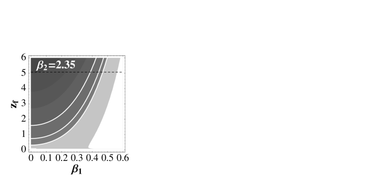
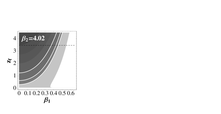
Figure 1: Curves at constant $\sigma_{8}$ (from eq. (76)), and $\beta{{}_{2}}$ fixed at the values 2.35 (top) and $4.02$ (bottom). The allowed region is below the dashed line, and within the upper and lower white curves, corresponding to the limiting values of eq. (77).

The plots of Fig. 1 refer to our “phenomenological” set of parameters, and in particular to the duration of the freezing epoch (possibly relevant to the solution of the coincidence problem). The $\sigma_{8}$ constraint provides however interesting information also on the set of “fundamental” parameters of the string effective action (1), used for our model of dilatonic dark energy.

By eliminating $c_{1}/c_{2}=\sqrt{2/3}\mu_{2}$, and fixing $q_{0}$, i.e. $\beta{{}_{2}}$, as before, we can plot indeed the $\sigma_{8}$ constraint in the plane spanned by the variables $c^{2}$ and $V_{0}$. The result is shown in Fig. 2, again for $\beta{{}_{2}}=2.35$ (left panel) and for $\beta{{}_{2}}=4.02$ (right panel). We have restored the required Planck length factors, and given the potential $V_{0}$ in units of ${\textrm{eV}}^{4}$. The allowed region is within the upper and lower white curves, as before. The lower bound on $c^{2}$ derived from $\beta{{}_{1}}$, at fixed $\beta{{}_{2}}$, is satisfied for all the range of values illustrated in the picture.

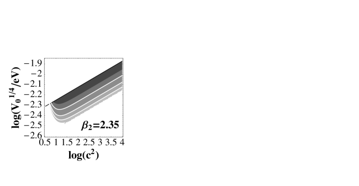
Figure 2: Curves at constant $\sigma_{8}$, and $\beta{{}_{2}}$ fixed at the values 2.35 (top) and $4.02$ (bottom). The allowed region is below the straight line representing the consistency bound $z_{f}<z_{b}$, and within the upper and lower white curves corresponding to the limiting values of eq. (77).

We note that the values of parameters used in GPV01 for a particular numerical integration of the string cosmology equations are well compatible with the above bounds. It is also important to stress that, since the value of $c^{2}$ is naturally expected in the range $10^{2}$–$10^{3}$ GPV01 , the allowed mass scale of the dilaton potential, $V_{0}^{1/4}$, turns out to be fixed in a rather narrow region around ($10^{-2}$–$10^{-3}$) eV, even in the case of an early start of the freezing epoch. This result confirms that, as already pointed out in GPV01 , a realistic dark-energy scenario seems to require a rather high degree of accuracy in determining the scale of the dilaton potential. This (fine-tuning?) aspect of the potential is however a common problem of all scalar-field models of dark energy.

It should be mentioned, to conclude this section, that we have performed an additional observational test of our class of dilatonic dark-energy models by comparing with the COBE data the slope of the low-multipole $C_{\ell}$ spectrum induced by the SW and ISW effect. Using a simple Gaussian likelihood distribution we have concluded that, at the confidence level of two sigma, the predicted slopes are compatible with the data for all the allowed region of parameter space, so that no (significant) additional constraints are generated.

V The farthest supernova

As a last check on the viability of the present dilatonic dark-energy model we have considered the constraints imposed by the most distant Type Ia supernova super known so far, SN1997ff, for which a very recent assessment of lensing magnification has increased the apparent magnitude by $0.34\pm 0.12$ mag super1 . This leads to a final distance modulus (i.e. to a difference of apparent and absolute magnitude) of $m-M=45.49\pm 0.34$ mag.

Using the definition adopted in super , this result can be expressed in the following way. The luminosity distance is

$$d_{L}=(1+z)\int_{0}^{z}\frac{dz^{\prime}}{H(z^{\prime})},$$ (80)

from which one defines

$$\Delta(m-M)=5[\log_{10}(d_{L}(z))-\log_{10}(d_{L\circ}(z))],$$ (81)

where $d_{L\circ}(z)=z(z+2)/(2H_{0})$ is the luminosity distance for Milne’s model, i.e. an hyperbolic empty universe ($\Omega_{m}=\Omega_{\Lambda}=0$). For the supernova SN1997ff one obtains $\Delta(m-M)\approx-0.15\pm 0.34$ at $z\approx 1.755$, in good agreement with a $\Lambda$CDM model characterized today by $\Omega_{m}=0.35,\Omega_{\Lambda}=0.65$ super1 . For such a model, the Universe at $z=1.755$ is already well within the decelerated epoch, which starts around $z=0.548$ (see eq. 79).

This does not imply, however, that all models which are accelerated at large $z$ are ruled out (even without mentioning the still unclear experimental uncertainties of such a supernova detection). Let us calculate indeed the luminosity-distance along a stationary regime $\rho_{m}\sim\rho_{\phi}$, for a spatially flat geometry. Neglecting for the moment the baryon contribution, the Friedmann equation is

$$H^{2}=H_{0}^{2}\left[\Omega_{m}(a/a_{0})^{-3w}+\Omega_{\phi}(a/a_{0})^{-3w}\right]=H_{0}^{2}(a/a_{0})^{-3w},$$

where, in particular, $w=w_{2}$ (see eq. 27) for our freezing regime. The corresponding luminosity-distance (for $w\not=2/3)$ is:

$$d_{L}=(1+z)\int_{0}^{z}\frac{dz^{\prime}}{H(z^{\prime})}=\frac{2(1+z)}{(2-3w)H_{0}}\left[(1+z)^{-\frac{3w}{2}+1}-1\right].$$ (82)

For an accelerated evolution with $w<2/3$ (i.e., in our case, $q_{0}>1$), and for large $z$, we have $d_{L}\sim z^{2-3w/2}$, while for Milne’s cosmology $d_{L}\sim z^{2}.$ It follows that, at large $z$ and for any $w>0$, the Milne model always provides larger distances (and thus larger apparent magnitudes) than a model of stationary evolution. As a consequence, a negative value of $\Delta(m-M)$, referred to Milne, does not necessarily corresponds to deceleration.

For a more precise illustration of this important point we have plotted in Fig. 3 the distance modulus $\Delta(m-M)$ for the accelerated freezing phase of our dilatonic dark-energy model. We have numerically integrated the luminosity-distance functions, including baryons, for the two particular values $\beta_{2}=2.35,\beta_{2}=4.02$ already used in the previous figures (it may be useful to recall that, when $\Omega_{c}$ is fixed to $0.3$, these two values of $\beta{{}_{2}}$ correspond to $w_{2}=0.5$ and $w_{2}=0.4$, respectively). It can be seen from the picture that, in both cases, the curves representing the cosmic evolution of our model, although deeply inside the accelerating regime, remain well within one sigma from the (lensing-corrected) SN1997ff data, while providing, at the same time, a reasonable fit of the binned data of all the other supernovae.

Figure 3: The distance modulus $m-M$, referred to Milne’s cosmology, for a $\Lambda$CDM model (dashed curve) and for dilatonic dark-energy model during the freezing epoch, for two values of $\beta_{2}$ (thick curves when baryons are included, thin curves without baryons). The points at $z<1$ represent the binned data from all the high-redshift Ia supernovae known so far. The datum plotted at $z=1.755$ represents the lensing-corrected SN1997ff . All data are derived from super ; super1 .

VI Conclusion

In this paper we have considered a phenomenological model of dark-energy-dark-matter interactions based on the infinite bare-coupling limit of the superstring effective action. The dilaton, rolling down an exponentially suppressed potential, plays the role of the cosmic field responsible for the observed acceleration, and drives the Universe towards a final configuration dominated by a comparable amount of kinetic, potential and CDM energy density.

The effective dilatonic coupling to dark matter switches on at late enough times (i.e., large enough bare coupling), and affects in a significant way the post-equivalence cosmological evolution. The time-dilution of the dark-matter density, in particular, is first slightly enhanced (during the dragging phase) and then considerably damped (during the freezing phase) with respect to the standard $a^{-3}$ decay law. The large-angle fluctuation scales relevant to the observed CMB anisotropies reenter the horizon during the dragging epoch, and exit the horizon again during the freezing epoch. In spite of this unconventional evolution, the growth of the matter-density perturbations may be large enough to match consistently present observations.

The predicted value of the (smoothed out) density contrast $\sigma_{8}$, compared with data obtained from cluster abundance, defines a significant allowed region in the parameter space of the given class of dilatonic dark-energy models. The analysis of such an allowed region provides two main results.

The first is that the bounds on the past-time extension of the accelerated (freezing) epoch are significantly weaker than in conventional dark-energy models (uncoupled to dark matter, with frozen equation of state). The establishment of the freezing regime, in our class of dilatonic models, is allowed long before the present epoch (up to $z\simeq 5$), thus providing (in principle) a further relaxation of the coincidence problem, by extending the present cosmological configuration not only in the far future, but also towards the past.

The possibility of very early ($z>1$) accelerated evolution is indeed a typical signature of such a class of dilatonic models, useful in principle to discriminate it from other (uncoupled) dark energy models, hopefully on the grounds of future observational data. It is important to stress, to this respect, that the farthest type Ia supernova so far observed is at $z\simeq 1.7$, and is perfectly compatible with an accelerated Universe already at that epoch, provided the data of the magnitude-redshift diagram are consistently fitted by the accelerated kinematics of dilatonic models.

The second results concerns the parameters of the (non-perturbative) dilaton potential appearing in the strong-bare-coupling regime of the string effective action. The dilaton mass scale $V_{0}$, for an efficient and realistic dark energy scenario, appears in such a context to be tightly anchored to a value very near to the present Hubble curvature scale. A small deviation of $V_{0}$ from the required value is enough to remove the predictions of the dilatonic model from the region of parameter space allowed by the $\sigma_{8}$ data.

This means that, under the assumption that the dilatonic models discussed in this paper provide the correct explanation of the observed cosmic acceleration, the measurements of the density contrast $\sigma_{8}$, besides their obvious astrophysical importance, would also acquire an interesting high-energy significance for providing an indirect (parameter-dependent) measurements of the dilaton mass scale.

We note, finally, that astrophysical observations may provide several additional constraints on dilatonic dark-energy models. For instance, the clustering evolution of sources at high redshifts may constrain directly the freezing growth exponent $m_{2}$; as already mentioned, the baryon bias that develops during freezing is also observable, at least in principle bias ; finally, further constraints can be derived from a computation of the full multipole spectrum of the CMB radiation (see e.g. aqtp for a recent study of the CMB constraints on coupled dark-energy models with power-law potentials). Preliminary results seem to confirm the conclusions of this paper, but a detailed discussion of these new constraints is postponed to a future work.

- (1) A. G. Riess et al, Astron. J. 116, 1009 (1998).
- (2) S. Perlmutter et al, Ap. J. 517, 565 (1999).
- (3) A. T. Lee et al., Ap. J. 561, L1 (2001).
- (4) C. B. Netterfield et al., astro-ph/0104460.
- (5) J. Frieman, C. T. Hill, A. Stebbins and I. Waga, Phys. Rev. Lett. 75, 2077 (1995).
- (6) C. Wetterich, Astronomy and Astrophys. 301, 321 (1995).
- (7) A. Albrecht, F. Burgess, F. Ravndal, and C. Skordis, astro-ph/0107573.
- (8) M. Gasperini, Phys. Rev. D 64, 043510 (2001).
- (9) M. Gasperini, F. Piazza and G. Veneziano, Phys. Rev. D65, 023508 (2001).
- (10) M. Pietroni, hep-ph/0203085.
- (11) P. Steinhardt, in Critical problems in Physics, edited by by V. L. Fitch and D. R. Marlow (Princeton University Press, Princeton, NJ, 1997).
- (12) A. Riess et al. Ap. J. 560, 49 (2001).
- (13) N. Benitez et al., astro-ph/0207097.
- (14) L. Amendola and D. Tocchini-Valentini, Phys. Rev. D64, 043509 (2001).
- (15) L. Amendola & D. Tocchini-Valentini, astro-ph/0111535.
- (16) M. B. Green, J. Schwartz and E. Witten, Superstring Theory (Cambridge Univ. Press, Cambridge, England, 1987).
- (17) G. Veneziano, , JHEP 0206, 051 (2002).
- (18) V. Kaplunovsky, Phys. Rev. Lett. 55, 1036 (1985).
- (19) M. Gasperini, Phys. Lett. B470, 67 (1999).
- (20) T. Damour, F. Piazza and G. Veneziano, gr-qc/0204094; hep-th/0205111.
- (21) L. Amendola, Phys. Rev. D62, 043511 (2000).
- (22) D. Tocchini-Valentini and L. Amendola, Phys.Rev. D65, 063508 (2002)
- (23) R. R. Caldwell, R. Dave and P. J. Steinhardt, Phys. Rev. Lett. 80, 1582 (1998).
- (24) C. Armendariz-Picon, V. Mukhanov and P. J. Steinhardt, Phys. Rev. Lett. 85, 4438 (2000).
- (25) M. Doran, J. M. Schwindt and C. Wetterich, Phys. Rev. D64, 123520 (2001).
- (26) N. Dalal et al., Phys. Rev. Lett. 87, 141302 (2001).
- (27) W. Hu and M. White, Astron. Astrophys. 315, 33 (1995).
- (28) E.W. Kolb and M. S. Turner, The Early Universe (Addison-Wesley, 1990).
- (29) W. Hu and N. Sugiyama, Ap. J. 471, 542 (1996).
- (30) E. F. Bunn and M. White, Ap.J. 480, 6 (1997).
- (31) P. T. P. Viana and A. R. Liddle, MNRS 303, 535 (1999); M. Girardi, S. Borgani, G. Giuricin, F. Mardirossian and M. Mezzetti, Ap. J. 506, 45 (1998).
- (32) O. Lahav et al., astro-ph/0112162.
- (33) S. Burles, K. M. Nollett and M. S. Turner, Ap. J. 552, L1 (2001).
- (34) L. Amendola, C. Quercellini, D. Tocchini-Valentini and A. Pasqui, astro-ph/0205097.