Gravity-driven Turbulence in Galactic Disks

Abstract

High-resolution, 2-D hydrodynamical simulations with a large dynamic range are performed to study the turbulent nature of the interstellar medium (ISM) in galactic disks. The simulations are global, where the self-gravity of the ISM, realistic radiative cooling, and galactic rotation are taken into account. In the analysis undertaken here, feedback processes from stellar energy source are omitted. We find that the velocity field of the disk in a non-linear phase shows a steady power-law energy spectrum over three-orders of magnitude in wave number. This implies that the random velocity field can be modeled as fully-developed, stationary turbulence. Gravitational and thermal instabilities under the influence of galactic rotation contribute to form the turbulent velocity field. The Toomre effective $Q$ value, in the non-linear phase, ranges over a wide range, and gravitationally stable and unstable regions are distributed patchily in the disk. These results suggest that large-scale galactic rotation coupled with the self-gravity of the gas can be the ultimate energy sources that maintain the turbulence in the local ISM. We find that our models of turbulent rotating disks are consistent with the velocity dispersion of an extended HI disk in the dwarf galaxy, NGC 2915, where there is no prominent active star formation. Numerical simulations show that the stellar bar in NGC 2915 enhances the velocity dispersion, and it also drives spiral arms as observed in the HI disk.

1 INTRODUCTION

Observational and theoretical studies have suggested that there are supersonic hydrodynamical or magneto-hydrodynamical turbulent motions in molecular clouds and also in various phases of the ISM (McCray & Snow, 1979; Larson, 1981; Quiroga, 1983; Balbus & Hawley, 1991; Goldreich & Sridhar, 1995, 1997; Franco & Carramiñana, 1999). A number of numerical studies showed, however, that the turbulence in the clouds decays as $t^{-\eta}$, with $\eta\sim 1$ (Mac Low et al., 1998; Ostriker, Stone, & Gammie, 2001). The dissipation time of the turbulence is of the order of the flow crossing time or smaller, even in the presence of strong magnetic fields (Stone, Ostriker, & Gammie, 1998). These numerical experiments suggest that energy input is necessary to maintain the turbulent motion in the molecular clouds. Some energy sources originating in stellar activity have been proposed: stellar winds from young stars (Norman & Silk, 1980), photoionization (McKee, 1989), and supernova explosions (McKee & Ostriker, 1977). However, these processes can not be the main energy sources for keeping the turbulent motion in molecular clouds that do not harbor stellar activities (Williams & Blitz, 1998). In this case, external shocks caused by distant stellar energy release may produce vortices in the clouds (Kornreich & Scalo, 2000).

In differentially rotating disks with a magnetic field, the magneto-rotational instability (Balbus & Hawley, 1991) is a probable cause for the turbulent motion. Sellwood & Balbus (1999) have studied the MHD turbulence in extended HI disks, applied their model to the extended HI disk of NGC 1058, and have showed that the observed uniform velocity dispersion may be modeled by the MHD-driven turbulence.

In terms of the origin of the non-self-gravitating, pure hydrodynamical turbulence, on the other hand, Balbus, Hawley and Stone (1996) have claimed, on the basis of theoretical and numerical studies, that Keplerian disks are linearly and non-linearly stable. They rejected self-sustained hydrodynamical turbulence with outward angular momentum transport, because the turbulence cannot gain energy from the differential rotation. However, Kato & Yoshizawa (1997) suggested a steady hydrodynamical turbulence in Keplerian disks, which are caused by the pressure-strain tensor. Richard & Zahn (1999) have re-analiezed laboratory experiments of the Couette-Taylor flow, and concluded that turbulence may be sustained by differential rotation when $d\Omega/dR<0$. Godon & Livio (1999) showed that purely hydrodynamical perturbations can develop initially into either sheared disturbances or coherent vortices (see also Papaloizou & Pringle 1985). However, the perturbations decay and do not evolve into a self-sustained turbulence.

Another important mechanism that generates turbulence in a rotating disk is self-gravitational, local or global instability of the gas (Goldreich & Lynden-Bell, 1965a, b). Although there are some simulations of self-gravitating, turbulent gas in a local shearing box (e.g. V$\acute{\rm{a}}$zquez-Semadeni et al. 1995; Gammie 2001), the local approximation would not be adequate to study the nature of self-gravity dominated turbulence (Balbus & Papaloizou, 1999). The global hydrodynamical simulations given by Laughlin, Korchagin & Adams (1998) have revealed spiral unstable modes in the differentially rotating disk, but the development of self-sustained turbulence was not observed.

In the this paper, we study the gravity-driven turbulence in galactic disks using two-dimensional, global hydrodynamical simulations. We solve the basic hydrodynamical equations and the Poisson equation numerically, taking into account realistic radiative cooling. We use the same numerical technique discussed by Wada & Norman (1999,2001) (hereafter WN99, WN01), in which kpc-scale dynamics of the multi-phase ISM can be followed with a sub-pc resolution. WN99 and WN01 suggested that a gravitationally unstable and thermally unstable disk can evolve into a globally quasi-stable disk with quasi-stationary turbulent velocity field. Here we perform simulations with a higher spatial resolution, and make a detailed analysis of the turbulent structure.

In §2, we briefly summarize the numerical method and models, and in §3, we show that turbulent energy spectra are achieved over a wide dynamic range (from kpc to pc) in the direct numerical experiments. In order to study the effects of pure turbulence in the disk, we here ignore the energy feedback due to supernovae and stellar winds from massive stars (Norman & Ferrara, 1996). In §4, we discuss what is required for realistic models of the ISM, and we apply our model to the HI disk of the dwarf galaxy, NGC 2915. Extended HI disks are particularly relevant objects to compare with our models, because they are not significantly affected by the star formation (Dickey, Hanson, & Helou, 1990; Meurer et al., 1996). We summarize our results in §5.

2 NUMERICAL METHODS AND MODELS

The numerical methods are the same as those described in WN99 and WN01. Here we summarize them briefly. We solved the following equations numerically in two-dimensions:

$$\frac{\partial\Sigma_{g}}{\partial t}+\nabla\cdot(\Sigma_{g}\mbox{\boldmath${v}$}) = 0,$$ (1)

$$\frac{\partial\mbox{\boldmath${v}$}}{\partial t}+(\mbox{\boldmath${v}$}\cdot\nabla)\mbox{\boldmath${v}$}+\frac{\nabla p}{\Sigma_{g}} = -\nabla\Phi_{\rm ext}-\nabla\Phi_{\rm sg},$$ (2)

$$\frac{\partial E}{\partial t}+\frac{1}{\Sigma_{g}}\nabla\cdot[(\Sigma_{g}E+p)\mbox{\boldmath${v}$}] = \Gamma_{\rm UV}-\Sigma_{g}\Lambda(T_{\rm g}),$$ (3)

$$\nabla^{2}\Phi_{\rm sg} = 4\pi G\Sigma_{g}\delta(z)$$ (4)

where, $\Sigma_{g},p,\mbox{\boldmath${v}$}$ are surface density, pressure, and velocity of the gas, the specific total energy $E\equiv|\mbox{\boldmath${v}$}|^{2}/2+pH/[(\gamma-1)\Sigma_{g}]$ with $\gamma=5/3$ and a scale height $H$. The potential has two parameters, $a$ (scale parameter called the ‘core radius’) and $v_{\rm max}$ (the maximum rotation speed), and is expressed as

$$\Phi_{0}(R)=\frac{c^{2}}{a{(R^{2}+a^{2})}^{1/2}}\ ,$$ (5)

where $c$ is given as $c\equiv v_{\rm max}{(27/4)}^{1/4}a$, with $v_{\rm max}=150$ km s^-1 and $a=$0.2 and 2 kpc.

We also assume a cooling function $\Lambda(T_{g})$ $(10<T_{g}<10^{8}{\rm K})$ with Solar metallicity and a heating due to photoelectric heating, $\Gamma_{\rm UV}$. A constant scale height ($H=100$ pc) is assumed to calculate the cooling rate. We assume a uniform UV radiation field, equal to the the local Galactic UV field (Gerritsen & Icke, 1997). However, the UV heating does not significantly affect the dynamics of the ISM.

The hydrodynamic part of the basic equations is solved by AUSM (Advection Upstream Splitting Method), (Liou & Steffen, 1993). We achieve third-order spatial accuracy with MUSCL (van Leer, 1977). The limiter function is chosen to satisfy the TVD (Total Variation Diminishing) condition. In this scheme, an explicit numerical viscous term is not required and shocks are captured sharply. We used $4096^{2}$ equally spaced Cartesian grid points covering a 2 kpc $\times$ 2 kpc region around the galactic center. We also run models using $1024^{2}$ and $2048^{2}$ grid points to evaluate how numerical resolution affects the results.

The Poisson equation is solved to calculate the self-gravity of the gas using the FFT and the convolution method (Hockney & Eastwood, 1981). The second-order leap-frog method is used for the time integration. We adopt implicit time integration for the cooling term.

The initial condition is an axisymmetric and rotationally supported disk assuming the Toomre’$Q$ parameter, $Q=1.2$. Random density and temperature fluctuations are added at each grid cell in the initial disk. These fluctuations are less than 1 % of the unperturbed values and have an approximately white noise (flat power spectrum) distribution.

3 RESULTS

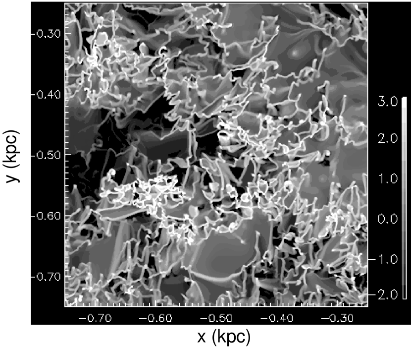
Figure 1: Density distribution of the gas in $1/16$ of the whole calculating region (2 kpc $\times$ 2 kpc) at $t=48.2$. $(x,y)=(0,0)$ is the galactic center. The gray scale represents log-scaled density ($M_{\odot}$ pc^-2).

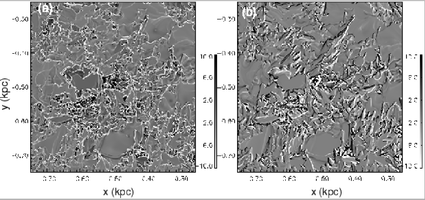
Figure 2: (a) Divergence of the velocity field ($\nabla\cdot\mbox{\boldmath${v}$}$) in the same area of Fig. 1. (b) Same as (a), but for $z$-component of rotation, i.e. $(\nabla\times\mbox{\boldmath${v}$})_{z}$. The unit is km s^-1 pc^-1.

As described in WN01, thermal and gravitational instabilities grow non-linearly over the whole of the disk in a few dynamical time scales. The whole system shows a quasi-stable state after $t\sim 20$ Myr (2 rotational periods at $R=0.2$ kpc). As shown in Fig. 1, which is a density field of a part of the disk (500 pc $\times$ 500 pc, i.e. 1/16 of the entire simulated region), a complicated network of clumps and filaments as well as low density voids are formed. The density ranges from $10^{-4}$ to $10^{6}$ $M_{\odot}$ pc${}^{-2}\,$. The velocity field in the same region in Fig. 1 is also very complicated as shown in Fig. 2a and 2b, in which $\nabla\cdot\mbox{\boldmath${v}$}$ and $(\nabla\times\mbox{\boldmath${v}$})_{z}$ are plotted. Comparing to Fig. 1 and 2, we see that regions of converging velocity roughly coincide with dense filaments, and positive and negative vortices are also associated with the filaments. This shows that local shearing motions are generated along the filaments. One should note that this turbulent velocity field is maintained in a rotating, self-gravitating gas disk without any explicit energy inputs, such as supernovae or any other artificial driving forces.

In order to understand the nature of the turbulent velocity field statistically, we calculate the energy spectra, $E(k)$ from the velocity field, where $k$ is the wave number. We decompose the velocity field into two components, i.e. $\mbox{\boldmath${v}$}=\mbox{\boldmath${v}$}_{\rm comp}+\mbox{\boldmath${v}$}_{\rm sol}$, where $\mbox{\boldmath${v}$}_{\rm comp}$ is the compressible velocity field and $\mbox{\boldmath${v}$}_{\rm sol}$ is the incompressible (or solenoidal) field (Passot, Pouquet, & Woodward, 1988). The two components are defined from $\nabla\cdot\mbox{\boldmath${v}$}_{\rm sol}=0$ and $\nabla\times\mbox{\boldmath${v}$}_{\rm comp}=0$, and solenoidal and compressible energy spectra, $E_{s}(k)$ and $E_{c}(k)$ are calculated from $\mbox{\boldmath${v}$}_{\rm sol}$ and $\mbox{\boldmath${v}$}_{\rm comp}$, respectively. Figure 3a shows the evolution of the compressible energy spectrum, $E_{c}(k)$. One finds that the compressible part of the velocity field reaches a quasi-steady state in a few rotational periods, where the spectrum shows a double power-law shape with a ‘knee’ at $k\sim 300$ ($\lambda\sim 7$ pc). The kinetic energy is mainly driven at wavenumbers around $k_{i}\sim 200-300$. The turbulence inversely cascades to a larger scale ($k\lesssim 100$), and simultaneously it also cascades to smaller scales. The input wave number, $k_{i}$, corresponds to about 10 pc, which is the scale of the initial gravitational instability in the cool phase after the initial cooling. The inverse cascade implies a hierarchical growth of the gravitational instability in the disk. The energy spectrum of the solenoidal component $E_{s}(k)$ similarly evolves as that $E_{c}(k)$ does (Fig. 3b), but it has more power especially on the large scale ($k\lesssim 10$ or $\lambda\gtrsim 200$ pc) because of the galactic rotation. The appearance of the ‘hump’ at $k\sim 200$ at $t=1$ Myr and the following evolution suggest that eddies are generated on the same scale as the gravitational instability, and they propagate toward large and small scales. The rotational energy on a larger scale cascades downward at $k\sim 10$. This process is just like evolution of the gravitational instability in a rotating disk (Goldreich & Lynden-Bell, 1965a, b). We discuss this below.

A stationary power-law regime in the energy spectrum of the system implies a fully-developed turbulence, and its power-law index represents some statistical aspects of the turbulence. Before discussing the power-law indices and the range of the inertial cascade, we first check the simulation for numerical artifacts. Since the turbulence of the ISM is a phenomenon over a wide dynamic range, one should be careful about fitting the numerically obtained spectrum with a power-law. We are using a non-adaptive Eulerian grid, therefore the results on smaller scales can be affected by the numerical resolution. We therefore check the dependence of the turbulent spectrum on the resolution by using $2048^{2}$ and $1024^{2}$ grid points as well as the $4096^{2}$ grid points (i.e. 0.49 pc resolution). In Fig. 4, $E(k)=E_{s}(k)+E_{c}(k)$ for three cases using $4096^{2},2048^{2},$ and $1024^{2}$ grid points at $t=20.2$ are plotted. We find that 1) the three runs coincide at $k\lesssim 100$ within a factor of two, 2) the slopes of the ‘inertial ranges’ are the same $d{\rm ln}E(k)/d{\rm ln}k\sim-0.8$, and 3) the power-law indices of the ‘dissipation regions’ in the all three models approach to $\sim-5.2$. The positions of the ‘knees’ are shifted by about factor of two, therefore the inertial range is increased by a factor of two if we use twice the number of grid points. Therefore, we can safely conclude that the slope of the inertial range is not strongly affected by the spatial resolution.

In fully developed Kolmogorov incompressible turbulence, the steady power-law energy spectrum indicates a steady energy flow from large scales toward smaller scales. In two-dimensional, incompressible, hydrodynamical turbulence, stationary spectra are found to be proportional to $k^{-3}$ for $k>k_{f}$ (enstrophy, (i.e. squared vorticity) cascade regime) and to $k^{-5/3}$ for $k<k_{f}$ (energy ‘inverse’ cascade regime), where $k_{f}$ is the forcing wavenumber (Kraichnan, 1967). This inverse energy cascade is also observed in numerical simulations of a weakly compressible 2-D turbulence (Dahlburg et al., 1990). The evolution of the spectrum in Fig. 3a look consistent with the Kraichnan’s picture, with $k_{f}\sim 200$, although our spectrum is shallower ($d{\rm ln}E_{s}(k)/d{\rm ln}k\sim-1$) in the inertial range than the Kraichnan’s prediction.

In Fig. 5, the final energy spectra ($t=48$ Myr), $E(k)$, $E_{s}(k)$, and $E_{c}(k)$ for the model using $4096^{2}$ grid points are plotted. $E_{c}(k)$ has a power-law part $E_{c}(k)\propto k^{-0.8}$ between $k\sim 20$ and 200, and $E_{s}(k)\propto k^{-1}$ between $k\sim 10$ and 200. It is known that for shock-dominated, fully-developed turbulence, $E(k)\propto k^{-2}$, and for a weakly shocked turbulence, $E_{c}(k)\propto k^{-1.5}$ are expected (Passot, Pouquet, & Woodward, 1988). The present spectrum is shallower than these values, and it implies that the structure of velocity field is not determined only by shocks. However, it is not clear whether this difference originates from the complexity of the present system, i.e. a non-uniform, rotating, self-gravitating, and radiative turbulence. Even so, it is interesting that the resultant spectra in this complicated system show stationary power laws over inertial ranges as seen in the much simpler systems - uniform, non-selfgravitating, and non-radiative turbulence. Note that the slope will change if the simulations are generalized to include energy feedback from supernovae, which cause strong shocks in the ISM (WN01).

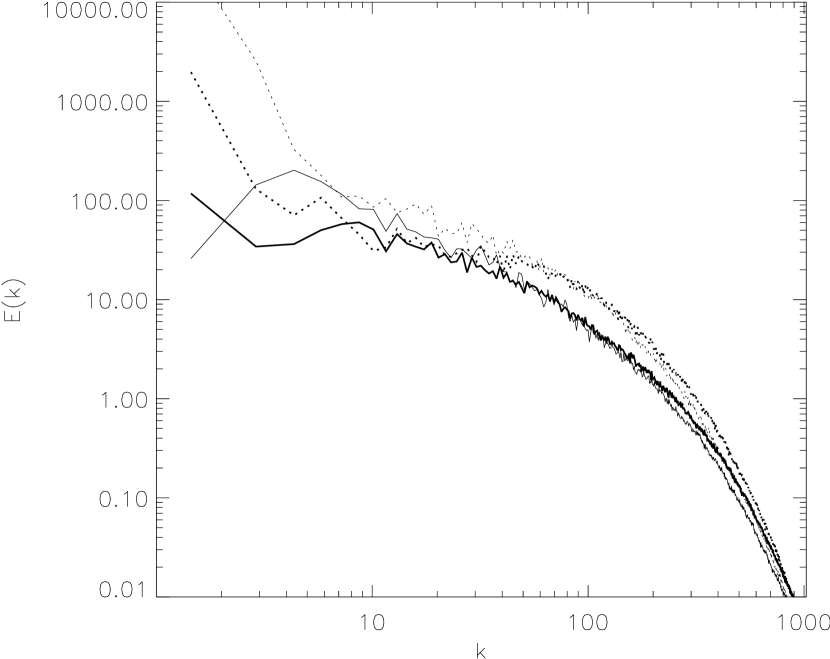
Figure 6: Energy spectra in two models with different rotation curves. The thick and thin solid lines are $E_{c}(k)$ and $E_{s}(k)$ for the ridge rotation (the core radius, $a=2$ kpc). The two dotted lines are the same, but for the differential rotation ($a=0.2$ kpc). The number of grid points are $2048^{2}$.

Next, we show energy spectra for two models with different rotation curves, i.e. rigid and differential rotation curves ($a=2$ and $a=0.2$ kpc) in Fig. 6. The plot shows that the spectra of the rigid rotation model on large scales ($k<10$) are smaller than those of the differential rotation model by a factor $10-100$. On the other hand, the difference of the spectra between the two models are a factor $2-3$ on small scales ($k>10$). Interestingly, the spectra of the inertial range in the rigid rotation model are steeper ($d{\rm ln}E(k)/d{\rm lnk}\sim-1.5$). It is reasonable that energy extracted from the galactic rotation is more effective when there is a shear field. We discuss this more quantitatively below.

The above numerical results suggest that the ISM in galaxies is dynamic, but in a statistical sense, it is in a ‘quasi-steady state’, whose velocity field resembles fully developed turbulence over a wide dynamic range (at least three orders of magnitude). The expected velocity dispersions are $\sim 10$ km s^-1 and 0.1 km s^-1 for 100 pc and 1 pc scales, respectively. There are two obvious energy sources that can maintain the turbulence in this system: the shear-driven by the galactic rotation and local tidal field due to the self-gravity of the gas. Besides these, local pressure gradients can also contribute to generate the turbulence. This is because that the turbulent ISM is no longer in pressure equilibrium (WN01, Gazol et al. 2001). As shown by the energy spectra (Fig. 5), the rotational energy is dominated by that on a large scale ($>200$ pc). On the other hand, turbulence is first driven by the self-gravity of the gas on a scale of 10–20 pc as seen in Fig. 3. These energy inputs are in equilibrium with the energy transport due to turbulent decay and losses due to the radiative cooling.

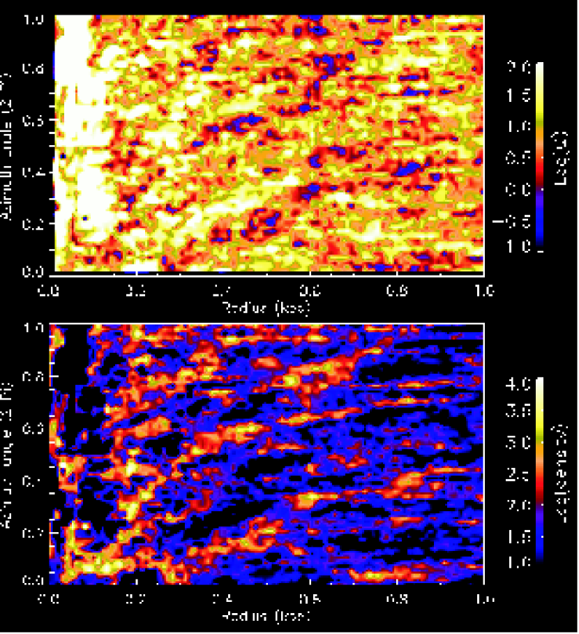
Figure 8: Two-dimensional distribution of the effective $Q(r,\phi)$ (upper panel) and the density $\Sigma_{g}(r,\phi)$ (lower panel) at $t=48$ Myr of the high resolution model ($4096^{2}$ zones). All quantities to calculate the effective $Q$, i.e. the epicyclic frequency, surface density and velocity dispersion are averaged in 100 $\times$ 60 sub-regions.

In order to see the effect of the gravitational instability on the generation of the turbulence, we calculate the effective Toomre stability parameter $Q\equiv\kappa\sigma_{e}/\pi G\Sigma_{g}$, where the effective velocity dispersion, $\sigma_{e}$, is defined by $\sigma_{e}^{2}\equiv\sigma^{2}+c_{s}^{2}$ with the velocity dispersion $\sigma$ and the sound velocity $c_{s}$, the average surface gas density $\Sigma_{g}$ and, the epicyclic frequency, $\kappa$. All quantities are averaged in local subregions (1 kpc$/\Delta R=100$ and $2\pi/\Delta\phi=60$). Fig. 7 shows the volume-weighted distribution functions of the $Q(R,\phi)$ for three different snapshots. It is notable that $Q$ is distributed over a wide range, i.e. four-orders of magnitudes. At $t=12.6$ Myr, a large fraction of the volume is in the unstable ($Q<1$) state. Note that, although the $Q<1$ implies that the axisymmetric mode is linearly unstable, the disk can be unstable to non-axisymmetric modes even with $Q>1$. The peaks shift to larger values for later times, which means the disk is stabilized. At $t=44.2$ Myr, the median is $Q\sim 5$, and the regions where $Q\ll 1$ and $Q\gg 1$ coexist. This situation is clearly seen in Fig. 8, which shows the 2-D distribution of $Q(R,\phi)$ and $\Sigma_{g}(R,\phi)$ at $t=44.2$ Myr. The distribution of the stable (yellow-white) and unstable regions (dark red-blue-black) are very patchy. It is obvious that the unstable regions correspond to high density regions, which are seen in the density map colored red-yellow. The disk is more unstable in the outer region ($R\gtrsim 0.5$ kpc) than in the inner region. The density map shows some global spiral structures, which can be also seen in the $Q$ map. The inhomogeneous distribution of $Q$ appears in the initial a few rotations, and then they evolve into larger structure. This evolution represents the development of the inhomogeneous structure in density, and the evolution of $E(k)$ as shown in Fig. 3 is consistent with this result. The most unstable wave length $\lambda_{m}$ in the differentially rotating disk is $\lambda_{m}\equiv 2\pi^{2}G\Sigma_{g}/\kappa^{2}\sim$3–30 pc. This is consistent with the typical size of the unstable regions seen in Fig. 8, which is less than about 50 pc. The sizes of the unstable regions are larger than those of the ’dissipational region’ seen in the energy spectra (Fig. 5), therefore the patchy structure is not strongly affected by the numerical resolution. The ISM in the $Q<1$ regions are expected to be collapsed, but this does not mean that all gas components in each unstable region eventually turn into one high density clump. In fact, there are substructures in the unstable regions, therefore due to the local angular momentum, the pressure gradient, and the Coriolis force, the collapse cannot be monotonic. As a result, the gravitational contraction causes the local velocity dispersion and shock heating, then the regions are stabilized. On the other hand, the stable regions can become unstable due to mass inflow and radiative cooling. Therefore the local structure of the stable and unstable regions are time-dependent, but the entire patchy structure seen in Fig. 8 does not change, which is consistent with fact that the energy spectra do not evolve significantly once the system reach the quasi-steady state.

The above results imply that the origin of the turbulent motion in the multi-phase, differentially rotating disk is gravitational instability. What we observe here is just like the ‘local’ gravitational instabilities in a rotating disk as discussed by Goldreich & Lynden-Bell (1965a,b), although the gas disks here have much more complicated multi-phase structures. The turbulence is driven by the gravitational instabilities, and probably it is also supplied by energy extracted from the galactic rotation. This is the same mechanism that drives the MHD turbulence. As discussed by Sellwood & Balbus (1999), the energy supply rate is given by $-T_{R\phi}d\Omega/d\ln R$, where the stress tensor is expressed using Alfven velocity $\mbox{\boldmath${u}$}_{A}$ and gravitational velocity $\mbox{\boldmath${u}$}_{G}$ as $T_{R\phi}=\langle\rho(u_{R}u_{\phi}-u_{AR}u_{A\phi}+u_{GR}u_{G\phi})\rangle$ (see also Lynden-Bell & Kalnajis 1972). Therefore, even if there is no magnetic field, the gravitational stress tensor works to extract energy from the galactic rotation.

The energy supply rate due to the gravitational instability per unit mass can be estimated as ${\dot{\varepsilon}}\sim\langle u_{GR}u_{G\phi}\rangle\Omega\sim G(\Sigma_{g}/H)\lambda^{2}\Omega\sim 5\Omega\,({\rm km\,s}^{-1})^{2}(\Sigma_{g}/10M_{\odot}{\rm pc}^{-2})(\lambda/100{\rm pc})^{2}(H/100\,{\rm pc})^{-1}$ (where $\lambda$ is a scale length of the turbulence) and $H$ is the scale height of the disk. The time scale of the energy supply, i.e. $v_{\rm rot}^{2}/{\dot{\varepsilon}}\sim(150\,{\rm km}\,{\rm s}^{-1})^{2}/5\Omega\sim 700\tau_{\rm rot}$, where $\tau_{\rm rot}$ is the rotational period, is long enough compared to the galactic life time. In other words, the turbulence can be sustained using a small fraction of the galactic potential energy. The dependence of the energy supply rate on the wavelength can be derived roughly as ${\dot{\varepsilon}}\sim G\Sigma_{g}/H\lambda^{2}\cdot Rd\Omega/dR\propto\lambda^{1/2}$ for the Kepler rotation ($\Omega\propto R^{-3/2}$) or ${\dot{\varepsilon}}\propto\lambda^{2}\Omega$ for the rigid rotation. Since the turbulent energy dissipation rate per unit mass should have the same dependence on the turbulent scale as the energy supply rate does, $v_{\rm turb}^{2}/(\lambda/v_{\rm turb})=v_{\rm turb}^{3}/\lambda\propto\lambda^{1/2}$, or $\propto\lambda^{2}$. As a result, we expect that $E(k)\propto k^{-1}$ for the Kepler rotation, or $E(k)\propto k^{-2}$ for the rigid rotation. That is, the power spectrum is steeper in the rigid rotation case than in the differentially rotating case as we see in Fig. 6. One should note that the turbulence extracts energy from the galactic rotation through self-gravity, and the galactic global shear is not a necessary condition to sustain the turbulence.

In addition to the local instability in self-gravitating disks, interactions with the non-axisymmetric disturbance, such as spiral density waves, can be a mechanism to redistribute energy from the background shear to the local disturbance through the $\langle u_{R}u_{\phi}\rangle$ term in the stress tensor (Lynden-Bell & Kalnajs, 1972; Papaloizou & Savonije, 1991; Laughlin, Korchagin & Adams, 1998). This has an analogy with the swing amplification of spiral density waves in differentially rotating, stellar disks (Julian & Toomre, 1966; Sellwood & Carlberg, 1984). As seen in Fig. 8, global spiral density waves evolve in the inhomogeneous disks after a few rotational times.

4 DISCUSSION

4.1 Towards more realistic modeling of the ISM

Modeling the ISM on a galactic scale is a challenging problem in numerical astrophysics. It is required that realistic simulations include many elementary processes, such as various radiative cooling/heating processes, thermal conduction, interaction between the magnetic field and the ISM, self-gravity of the gas, energy feedback from supernovae, etc. Moreover, the simulations should be ultimately three-dimensional and global, that is the whole galactic disk should be solved. In this sense, our model and any other past numerical simulations of the ISM are still highly idealized (see a review by V$\acute{\rm{a}}$zquez-Semadeni 2002). Our model is global, and realistic radiative cooling and self-gravity of the gas are taken into account, but the magnetic field, which is important for the evolution of the interstellar turbulence (see references in §1), is ignored. Therefore we should be careful to apply the present results to the real ISM. On the other hand, most MHD simulations of the ISM adopt the local shearing box approximation. There are many local 2-D models, e.g. self-gravitating ISM with radiative cooling (Vazquez-Semadeni et al. 1996), and self-gravitating ISM with isothermal or adiabatic equation of state (Kim & Ostriker, 2001; Gammie, 2001). Some models in 3-D consider radiative cooling and supernova feedback (Korpi et al., 1999), but most of them are local, non-selfgravitating, and an isothermal equation of state (EOS) is assumed (Mac Low, 1999). There was some global, 3-D MHD simulations with polytropic EOS calculated for the galactic central region, but they ignored self-gravity of the gas (e.g. Machida, Hayashi, & Matsumoto 2000). Using self-gravitating, global hydrodynamical simulations with radiative cooling, on the other hand, Wada (2001) showed that the ISM in the galactic central region has the complicated filamentary, multi-phase structure as seen in the 2-D simulations presented here. The results in the present paper and the past attempts are complementary, and they should be improved with more consistent numerical modeling of the ISM in the future.

Finally we would like to comment on plausibility of the 2-D approximation for the ISM. The real ISM in a galactic disk should behave as three-dimensional turbulence below the scale height of the cold gas ($\sim 100$ pc). Since the turbulence is driven by local gravitational instability, we expect that the ISM in 3-D behaves like 2-D turbulence on larger scales, therefore the inertial range of $d{\rm ln}E(k)/d{\rm ln}k\sim-1$ would also appear for $k\lesssim 40$ in 3-D ($k\lesssim 200$ in 2-D). For $k\gtrsim 40$, the energy spectrum would be Kolmogorov-like, i.e. $E(k)\propto k^{-5/3}$, or if it is shock-dominated, $E(k)\propto k^{-2}$ would be expected. In a real ISM on a smaller scale, the main energy sources would be magneto-hydrodynamical instability and/or energy feedback from stars as well as the energy decay from larger scales. Transition from 2-D to 3-D turbulence and its effect on the energy spectra are now important problems that can be addressed in studies of the gas dynamics in galactic disks, This would be clarified utilizing three-dimensional, global simulations of the ISM with magnetic field on a galactic scale.

One might wonder if the spatial resolution in our simulation is meaninglessly fine (i.e. $\sim 0.5$ pc), if we apply the model to the real ISM whose scale height is $\sim 100$ pc. However, as shown in Fig. 4, the transition from the inertia range to the ‘dissipative’ part is affected by the numerical resolution. The maximum wave length of the inertia range is about 10 times larger than the grid size. Therefore even for 2-D simulations, the spatial resolution should be much finer than the assumed scale heigh of the disk.

4.2 Origin of Velocity Dispersion in the HI Disk of NGC 2915

The HI disk in the dwarf galaxy, NGC 2915, extends to over five times the Holmberg radius, and there is no active star formation observed outside the central region. Therefore, this galaxy is relevant to our study of the dynamics of the turbulent gas disk without the influence of the stellar energy feedback. Meurer, Mackie, & Carignan (1994) and Meurer et al. (1996) observed NGC 2915 ($D=5.3$ Mpc, $M_{B}=-15.9$ mag, $R_{\rm Ho}=2.93$ kpc) using the ATCA (Australia Telescope Compact Array) with a linear resolution is 640 pc and the AAT (Anglo-Astrallia Telescope). The total mass of the HI disk is $9.6\times 10^{8}M_{\sun}$ and $R_{\rm HI}=14.9$ kpc. The integrated star-formation rate is 0.05 $M_{\sun}$ yr^-1, and most of the star-formation is near the center of the galaxy. The HI intensity map shows that there are spiral arms extending well beyond the optical extent. The isovelocity contours show that the disk is rotating with a small amount of non-circular motion. The line-of-sight velocity dispersion of the HI is $\sim 20-40$ km s^-1 inside the optical radius, and it is $\sim 8$ km s^-1 in the extended HI disk. The central question is what causes this large velocity dispersion in the extended HI disk?

We apply the same numerical method in §2 to model the HI disk in NGC 2915 to obtain the radial distribution of the velocity dispersion in a non-star forming disk. We scale the potential model (eq.(5)) and the gas disk to represent the HI disk of NGC 2915. Two rotation curves are assumed for an axisymmetric component of the external potential: 1) the potential derived from the HI rotation curve (Model A in Fig. 16 of Meurer et al. 1996), where the core radius $a$ in eq.(5) is 4 kpc, and 2) models with a smaller core radius ($a=2$ kpc). The latter model was chosen, because the HI rotation curves derived from tracing peak intensities of position-velocity maps do not necessarily represent true mass distribution of the galaxies, especially for the central part (Sofue et al., 1999). Sofue et al. (1999) claimed that the true central rotation curves tend to be steeper than those implied from the peak intensities in PV maps.

NGC 2915 has a central optical bar. The observed spiral patterns could be resonance-driven structures by this central bar. The velocity dispersion in the disk is generally enhanced by the non-axisymmetric potential and its resonances. The pattern speed of the bar can be directly measured (Tremaine & Weinberg, 1984), and it is $\Omega_{p}=8.0\pm 2.4$ km s^-1 kpc^-1 (Bureau et al., 1999). In order to investigate the effects of the central bar, we also performed runs with a non-axisymmetric potential (bar-potential) with the same pattern speed as observed (Bureau et al. 1999), and where the length of the bar is taken to be equal to the core radius $a$. The non-axisymmetric part of the potential is assumed to be in the form $\Phi_{1}(R,\phi,t)=\varepsilon(R)\Phi_{0}\cos 2(\phi-\Omega_{\rm p}t)\ ,$ where $\varepsilon(R)$ is given as $\varepsilon(R)=\varepsilon_{0}{aR^{2}}/{(R^{2}+a^{2})^{3/2}}.$ The parameter $\varepsilon_{0}$ represents the strength of the bar (Wada & Koda, 2001). The gas is initially distributed in an axisymmetric, 15 kpc radius disk with a exponential-like surface density profile to resemble the observed HI distribution (Fig. 15 in Meurer et al. 1996). We have run models with parameters as $6\leq\Omega_{p}\leq 11$ km s^-1 kpc^-1, $0.05\leq\epsilon_{0}\leq 0.15$, and $a=2$ and 4 kpc.

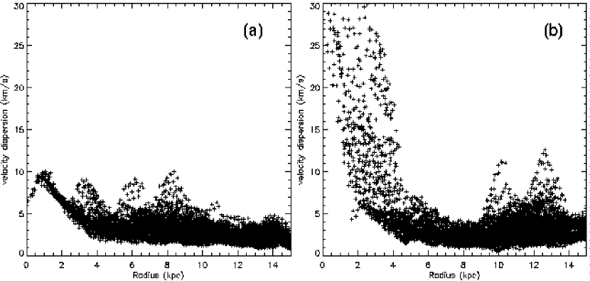
Figure 9: Radial distribution of the velocity dispersion for (a) axisymmetric model $A$, and (b) bar model $B$ for the extended HI disk of NGC 2915.

The velocity dispersions of an axisymmetric model $A$ ($a=4$ kpc) at $t=5.4$ Gyr are plotted as a function of the radius in Fig. 9a. The velocity field is sampled at every 20 grid points (i.e. 292 pc) for $x$ or $y$-directions, and they are averaged in the same size as the observed beam size to calculate the dispersion. We find that the dispersion is about a factor 4 smaller than the observed value (20-40 km s^-1) at $R<2$ kpc, a factor 2 smaller than the observed 8 km s^-1 at $R>2$ kpc. The velocity dispersions of a bar model $B$ ($a=2$ kpc, $\varepsilon_{0}=0.1,\Omega_{p}=8$ km s^-1 kpc^-1) is plotted in Fig. 9b. The central velocity dispersion in this model is $\sim 20-30$ km s^-1, and the it is about 3–4 km s^-1 in the outer disk. The central velocity dispersion is comparable with the observed value, but the dispersion in the outer disk is still factor 2 smaller than observations.

Fig. 10 shows $E(k)$ for the two models $A$ and $B$. Both spectra show double power-law shapes, $E(k)\propto k^{-1}$ and $k^{-1.5}$ in $10\lesssim k\lesssim 100$ for models $A$ and $B$, respectively. The slope of the axisymmetric model is comparable to that in Fig. 5. The steeper slope in the bar model would be due to stronger shocks caused by the bar. The spectra also shows that the bar model has a factor of 2-10 larger energy than the axisymmetric model in the most scales.

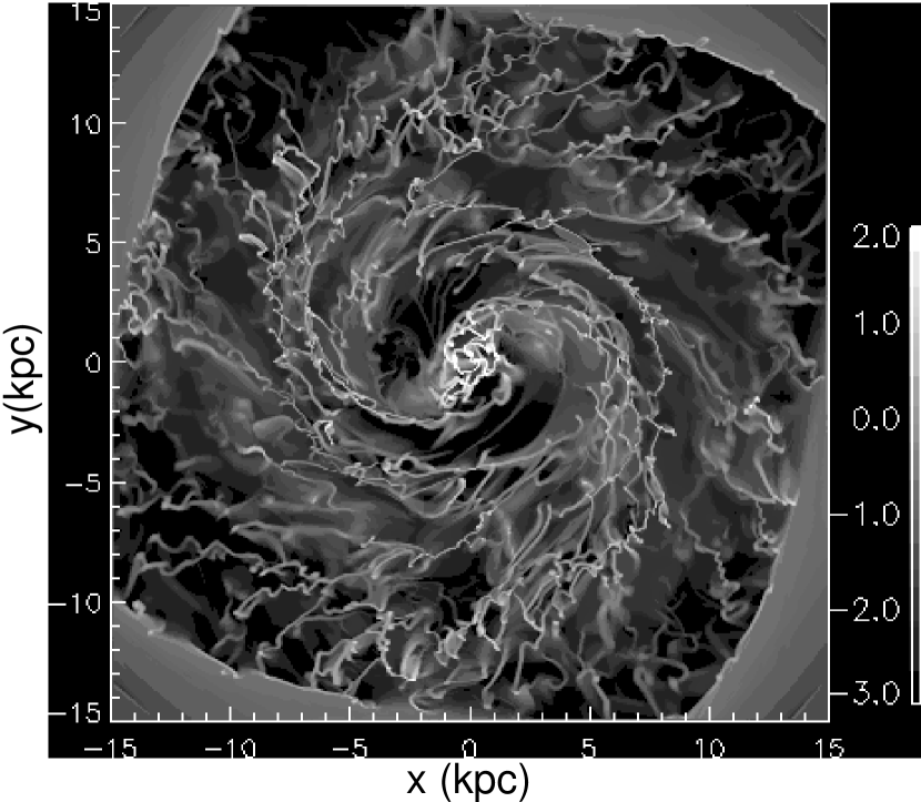
Figure 11: Density distribution of model $B$. The two major spirals are formed due to the outer Lindblad resonance, which is caused by the central stellar bar of the pattern speed 8 km s^-1 kpc^-1.

In Fig. 11 and 12, we plot the density and PV maps of the bar model $B$. Two major spiral arms, which are formed from many spirals and clumps, are evident as well as an inhomogeneous compact disk. The PV diagram shows a large velocity dispersion at $R<3$ kpc, which corresponds to the clumpy nuclear disk.

The Toomre’s $Q$ parameter estimated by the observations is 5–9 (Meurer et al., 1996). However, this does not mean that there are no local gravitationally unstable regions in the HI disk. The beam size in the observations is much larger than the typical size of the unstable regions. Therefore, we can observe the global stability of the HI disk, but probably the local instability is observed as the velocity dispersion in the beam size.

After exploring the parameter space ($\epsilon_{0},\,\Omega_{p}$, and $a$), we conclude that a set of parameters, i.e. $\epsilon_{0}\sim 0.1,\Omega_{p}\sim 8$ km s^-1 kpc^-1, and $a\sim 2$ kpc, reasonably reproduces the observed radial distribution of the velocity dispersion, and the HI morphology. However, the observed value of the velocity dispersion in the extended disk is about factor two larger than that in the best-fit model $B$. This might be due to the limitation of our model (§4.1), or because of the following reasons. Fig. 10 suggests that stronger bars can enhance the velocity dispersion in the disk by about factor of two. If the observed velocity dispersion is a result of hidden gravitational instability in the HI disk, the dispersion could be larger in a more massive disk. That is, the observed HI mass does not necessarily represent the total mass of the gas in the galaxy. There might be a component of high density, compact molecular clouds in the extended HI disk, which could be observed by the next-generation radio interferometer, ALMA.

5 SUMMARY

Dynamics and structure of the interstellar medium (ISM) in galactic disks are numerically studied, using high-resolution, 2-D hydrodynamical simulations with a large dynamic range. In §3, we showed that the velocity fields of the ISM in a steady-state show turbulent-like spectral energy distributions which are natural consequences of the non-linear development of gravitational instabilities of the ISM. The energy spectra are obtained over three-orders of magnitude in the wave number. The model using $4096^{2}$ grid points shows that the spectrum for the compressible and incompressible (solenoidal) part of the velocity field in the inertia ranges are fitted approximately as $E(k)\propto k^{-1.5}$ and $k^{-1}$, respectively. We found that the turbulent energy spectra are achieved in a few dynamical time-scales, and they subsequently remain in a quasi-steady state. We do not include energy feedback from supernovae or other external driving forces to produce and maintain turbulence. The turbulence is self-maintained over the wide dynamic range. From analyzing the temporal evolution of the energy spectra and the density structure, we suspect that energy input from self-gravitational interaction of the ISM and the galactic rotation drives the turbulence balancing the turbulent energy decay and the radiative cooling.

In §4, we compared our global ISM models with HI observations of NGC 2915. A large velocity dispersion ($\sim 8$ km s^-1) is observed in the extended HI disk of NGC 2915, even though there is no active star formation. We found that the observed velocity dispersion and its radial distribution in NGC 2915 can be quantitatively understood as the gravity-driven turbulence, but the galactic potential requires an additional non-axisymmetric potential with a rotation speed of $\Omega_{p}\sim 8$ km s^-1 kpc^-1 or the total gas mass should be larger than the observed HI mass.

Figure 3: (a) Evolution of energy spectrum for the compressible part of the velocity field, $E_{c}(k)$ is plotted for $t=0.2,1,2,3,4,8,16$, and 36 Myr. (b) Same as (a), but for the solenoidal part, $E_{s}(k)$.

Figure 4: Energy spectra, $E(k)=E_{s}(k)+E_{c}(k)$, for the three same models at $t=20.2$, but with different spatial resolutions: $4096^{2}$ (thick solid curve), $2048^{2}$ (thin solid curve), and $1024^{2}$ grid points are used (dotted curve). The six thin solid lines represent power-law whose slopes are -0.8 and -5.2.

Figure 5: Energy spectra, $E(k)$ (dotted line), $E_{s}(k)$ (dashed line), and $E_{c}(k)$ (solid line) of the high resolution model ($4096^{2}$ grid points are used) at $t=$ 48 Myr. The two thin solid lines represent power-laws of $k^{-1.5}$ and $k^{-0.8}$.

Figure 7: Histogram of the ’effective’ Toomre’s $Q$ parameter at $t=$ 12.6 (triangles), 25.6 (asterisks), and 44.2 Myr (crosses) of the high resolution model ($4096^{2}$ zones).

Figure 10: Energy spectra for the axisymmetric model $A$ (thin line) and for the bar model $B$ (thick line).

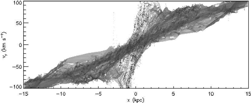
Figure 12: Position-Velocity ($x-v_{y}$) diagram of model $B$. The central high velocity components originate in the central clumpy disk seen in Fig. 11.

References

- Balbus, Hawley, & Stone (1996) Balbus, S. A., Hawley, J. F., & Stone, J. M. 1996, ApJ, 467, 76
- Balbus & Hawley (1991) Balbus, S. A. & Hawley, J. F. 1991, ApJ, 376, 214
- Balbus & Papaloizou (1999) Balbus, S. A. & Papaloizou, J. C. B. 1999, ApJ, 521, 650
- Bureau et al. (1999) Bureau, M., Freeman, K. C., Pfitzner, D. W., & Meurer, G. R. 1999, AJ, 118, 2158
- Dahlburg et al. (1990) Dahlburg, J. P., Dahlburg, R. B., Gardner, J. H., & Picone, J. M. 1990, Phys. Fluid, 2, 1481
- Dickey, Hanson, & Helou (1990) Dickey, J. M., Hanson, M. M., & Helou, G. 1990, ApJ, 352, 522
- Franco & Carramiñana (1999) Franco, J. & Carramiñana, A. 1999, Interstellar Turbulence, Cambridge Univ. Press, Cambridge
- Gazol et al. (2001) Gazol, A., Vázquez-Semadeni, E., Sánchez-Salcedo, F. J., & Scalo, J. 2001, ApJ, 557, L121
- Gammie (2001) Gammie, C. F. 2001, ApJ, 553, 174
- Gerritsen & Icke (1997) Gerritsen, J. P. E., Icke, V., 1997, A&Ap, 325, 972
- Godon & Livio (1999) Godon, P. & Livio, M. 1999, ApJ, 521, 319
- Goldreich & Lynden-Bell (1965a) Goldreich, P. & Lynden-Bell, D. 1965a, MNRAS, 130, 97
- Goldreich & Lynden-Bell (1965b) Goldreich, P. & Lynden-Bell, D. 1965b, MNRAS, 130, 125
- Goldreich & Sridhar (1995) Goldreich, P. & Sridhar, S. 1995, ApJ, 438, 763
- Goldreich & Sridhar (1997) Goldreich, P. & Sridhar, S. 1997, ApJ, 485, 680
- Hockney & Eastwood (1981) Hockney, R. W., Eastwood, J. W. 1981, Computer Simulation Using Particles (New York : McGraw Hill)
- Julian & Toomre (1966) Julian, W. H. & Toomre, A. 1966, ApJ, 146, 810
- Kato & Yoshizawa (1997) Kato, S. & Yoshizawa, A. 1997, PASJ, 49, 213
- Kim & Ostriker (2001) Kim, W. & Ostriker, E. C. 2001, ApJ, 559, 70.
- Kornreich & Scalo (2000) Kornreich, P. & Scalo, J. 2000, ApJ, 531, 366
- Korpi et al. (1999) Korpi, M. J., Brandenburg, A., Shukurov, A., & Tumominen, I. 1999, A&A, 350, 230
- Kraichnan (1967) Kraichnan, R. H. 1967, Phys. Fluids, 10, 1417
- Larson (1981) Larson, R. B. 1981, MNRAS, 194, 809
- Laughlin, Korchagin & Adams (1998) Laughlin, G., Korchagin, V., Adams, F.C., 1998, ApJ, 504, 945
- Liou & Steffen (1993) Liou, M., Steffen, C., 1993, J.Comp.Phys., 107,23
- Lynden-Bell & Kalnajs (1972) Lynden-Bell, D. & Kalnajs, A. J. 1972, MNRAS, 157, 1
- Mac Low et al. (1998) Mac Low, M., Klessen, R. S., Burkert, A., & Smith, M. D. 1998, Physical Review Letters, 80, 2754
- Mac Low (1999) Mac Low, M., ApJ 524, 169
- Machida, Hayashi, & Matsumoto (2000) Machida, M., Hayashi, M. R., & Matsumoto, R. 2000, ApJ, 532, L67.
- McCray & Snow (1979) McCray, R. & Snow, T. P. 1979, ARA&A, 17, 213
- McKee (1989) McKee, C. F. 1989, ApJ, 345, 782
- McKee & Ostriker (1977) McKee, C. F. & Ostriker, J.P. 1977, ApJ,218,148
- Meurer, Mackie, & Carignan (1994) Meurer, G. R., Mackie, G., & Carignan, C. 1994, AJ, 107, 2021
- Meurer et al. (1996) Meurer, G. R., Carignan, C., Beaulieu, S. F., & Freeman, K. C. 1996, AJ, 111, 1551
- Norman & Ferrara (1996) Norman, C. A., & Ferrara, A., 1996, ApJ, 467, 280
- Norman & Silk (1980) Norman, C. A., & Silk, J. 1980, ApJ, 238, 158
- Ostriker, Stone, & Gammie (2001) Ostriker, E. C., Stone, J. M., & Gammie, C. F. 2001, ApJ, 546, 980
- Passot, Pouquet, & Woodward (1988) Passot, T., Pouquet, A., & Woodward, P. 1988, A&A, 197, 228
- Papaloizou & Pringle (1985) Papaloizou, J. C. B. & Pringle, J. E. 1985, MNRAS, 213, 799
- Papaloizou & Savonije (1991) Papaloizou, J. C. B. & Savonije, G. J. 1991, MNRAS, 248, 353
- Quiroga (1983) Quiroga, R. J. 1983, Ap&SS, 93, 37
- Richard & Zahn (1999) Richard, D. & Zahn, J. 1999, A&A, 347, 734.
- Sellwood & Carlberg (1984) Sellwood, J. A. & Carlberg, R. G. 1984, ApJ, 282, 61
- Sellwood & Balbus (1999) Sellwood, J. A. & Balbus, S. A. 1999, ApJ, 511, 660
- Sofue et al. (1999) Sofue, Y., Tutui, Y., Honma, M., Tomita, A., Takamiya, T., Koda, J., & Takeda, Y. 1999, ApJ, 523, 136
- Stone, Ostriker, & Gammie (1998) Stone, J. M., Ostriker, E. C., & Gammie, C. F. 1998, ApJ, 508, L99
- Tremaine & Weinberg (1984) Tremaine, S. & Weinberg, M. D. 1984, ApJ, 282, L5
- van Leer (1977) van Leer, B., 1977, J.Comp.Phys., 32, 101
- Vazquez-Semadeni et al. (1995) Vzquez-Semadeni, E., Pasot, T. & Pouquet, A. 1995, ApJ, 441, 702
- Vazquez-Semadeni et al. (1996) Vzquez-Semadeni, E., Pasot, T. & Pouquet, A. 1996, ApJ, 473, 881
- Vazquez-Semadeni (2002) Vzquez-Semadeni, E. 2002, in “Seeing Through the Dust: The Detection of HI and the Exploration of the ISM in Galaxies”, eds. R.Taylor, T. Landecker, & A. Willis, ASP, San Francisco, in press (astro-ph/0201072)
- Wada (2001) Wada, K. 2001, ApJ, 559, L41
- Wada & Koda (2001) Wada, K. & Koda, J. 2001, PASJ, 53, 1163
- Wada & Norman (1999) Wada, K. & Norman, C. A. 1999, ApJ, 516, L13 (WN99)
- Wada & Norman (2001) Wada, K. & Norman, C. A. 2001, ApJ, 547, 172 (WN01)
- Williams & Blitz (1998) Williams, J. P. & Blitz, L. 1998, ApJ, 494, 657