ISO-SWS calibration and the accurate modelling of cool-star atmospheres

Vega, Sirius, $\beta$ Leo, $\alpha$ Car and $\alpha$ Cen A belong to a sample of twenty stellar sources used for the calibration of the detectors of the Short-Wavelength Spectrometer on board the Infrared Space Observatory (ISO-SWS). While general problems with the calibration and with the theoretical modelling of these stars are reported in Decin et al. (2002), each of these stars is discussed individually in this paper. As demonstrated in Decin et al. (2002), it is not possible to deduce the effective temperature, the gravity and the chemical composition from the ISO-SWS spectra of these stars. But since ISO-SWS is absolutely calibrated, the angular diameter ($\theta_{d}$) of these stellar sources can be deduced from their ISO-SWS spectra, which consequently yields the stellar radius (R), the gravity-inferred mass (M_g) and the luminosity (L) for these stars. For Vega, we obtained $\theta_{d}$$=3.35\pm 0.20$ mas, R$=2.79\pm 0.17$ R_⊙, M${}_{g}=2.54\pm 1.21$ M_⊙ and L$=61\pm 9$ L_⊙; for Sirius $\theta_{d}$$=6.17\pm 0.38$ mas, R$=1.75\pm 0.11$ R_⊙, M${}_{g}=2.22\pm 1.06$ M_⊙ and L$=29\pm 6$ L_⊙; for $\beta$ Leo $\theta_{d}$$=1.47\pm 0.09$ mas, R$=1.75\pm 0.11$ R_⊙, M${}_{g}=1.78\pm 0.46$ M_⊙ and L$=15\pm 2$ L_⊙; for $\alpha$ Car $\theta_{d}$$=7.22\pm 0.42$ mas, R$=74.39\pm 5.76$ R_⊙, M${}_{g}=12.80^{+24.95}_{-6.35}$ M_⊙ and L$=14573\pm 2268$ L_⊙ and for $\alpha$ Cen A $\theta_{d}$$=8.80\pm 0.51$ mas, R$=1.27\pm 0.08$ R_⊙, M${}_{g}=1.35\pm 0.22$ M_⊙ and L$=1.7\pm 0.2$ L_⊙. These deduced parameters are confronted with other published values and the goodness-of-fit between observed ISO-SWS data and the corresponding synthetic spectrum is discussed.

Appendix A Comparison between different ISO-SWS and synthetic spectra (coloured plots)

In this section, Fig. LABEL:acenvers – Fig. LABEL:acar, Fig. LABEL:bleovers – Fig. LABEL:vega of the accompanying article are plotted in colour in order to better distinguish the different observational or synthetic spectra.

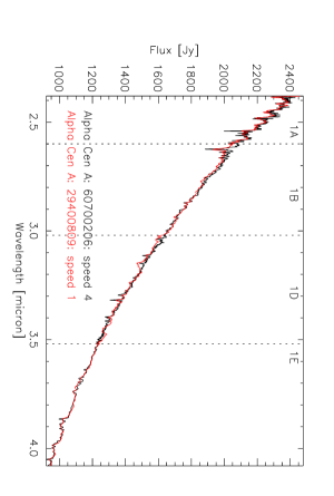
Figure 1: Comparison between the AOT01 speed-4 observation of $\alpha$ Cen A (revolution 607) and the speed-1 observation (revolution 294). The data of the speed-1 observation have been multiplied by a factor 1.16.

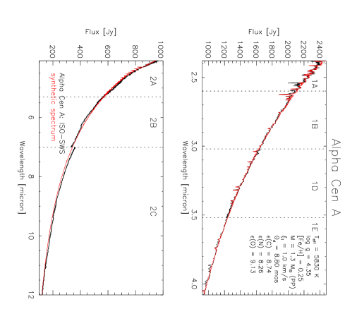
Figure 2: Comparison between band 1 and band 2 of the ISO-SWS data of $\alpha$ Cen A (black) and the synthetic spectrum (red) with stellar parameters T_eff = 5830 K, $\log$ g = 4.35, M = 1.3 M_⊙, [Fe/H] = 0.25, $\xi_{t}$ = 1.0 km s^-1, $\varepsilon$(C) = 8.74, $\varepsilon$(N) = 8.26, $\varepsilon$(O) = 9.13 and $\theta_{d}$ = 8.80 mas.

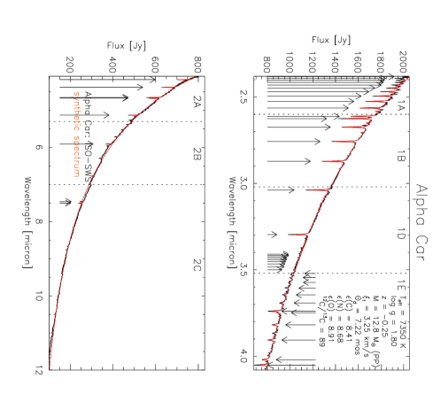
Figure 3: Comparison between band 1 and band 2 of the ISO-SWS data of $\alpha$ Car (black) and the synthetic spectrum (red) with stellar parameters T_eff = 7350 K, $\log$ g = 1.80, M = 12.8 M_⊙, [Fe/H] = $-0.25$, $\xi_{t}$ = 3.25 km s^-1, $\varepsilon$(C) = 8.41, $\varepsilon$(N) = 8.68, $\varepsilon$(O) = 8.91 and $\theta_{d}$ = 7.22 mas. Hydrogen lines are indicated by arrows.

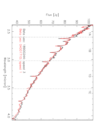
Figure 4: Comparison between the AOT01 speed-3 observation of $\beta$ Leo (revolution 189) and the speed-1 observation (revolution 040). The data of the speed-1 observation have been multiplied by a factor 1.05.

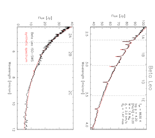
Figure 5: Comparison between band 1 and band 2 of the ISO-SWS data of $\beta$ Leo (black) and the synthetic spectrum (red) with stellar parameters T_eff = 8630 K, $\log$ g = 4.20, M = 1.8 M_⊙, [Fe/H] = 0.20, $\xi_{t}$ = 2.0 km s^-1 and $\theta_{d}$ = 1.47 mas.

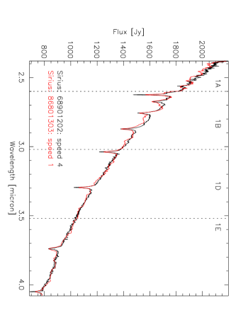
Figure 6: Comparison between the AOT01 speed-4 observation of $\alpha$ CMa (revolution 689) and the speed-1 observation (revolution 868). The data of the speed-1 observation have been multiplied by a factor 1.12.

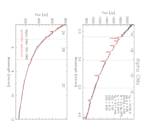
Figure 7: Comparison between band 1 and band 2 of the ISO-SWS data of $\alpha$ CMa (black) and the synthetic spectrum (red) with stellar parameters T_eff = 10150 K, $\log$ g = 4.30, M = 2.2 M_⊙, [Fe/H] = 0.50, $\xi_{t}$ = 2.0 km s^-1, $\varepsilon$(C) = 7.97, $\varepsilon$(N) = 8.15, $\varepsilon$(O) = 8.55 and $\theta_{d}$ = 6.17 mas.

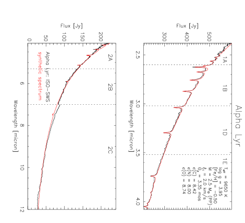
Figure 8: Comparison between band 1 and band 2 of the ISO-SWS data of $\alpha$ Lyr (black) and the synthetic spectrum (red) with stellar parameters T_eff = 9650 K, $\log$ g = 3.95, M = 2.5 M_⊙, [Fe/H] = $-0.50$, $\xi_{t}$ = 2.0 km s^-1, $\varepsilon$(C) = 8.42, $\varepsilon$(N) = 8.00, $\varepsilon$(O) = 8.74 and $\theta_{d}$ = 3.35 mas.

A

A

A

Appendix B Comments on published stellar parameters

In this appendix, a description of the results obtained by different authors using various methods is given in chronological order. One either can look to the quoted reference in the accompanying paper and than search the description in the chronological (and then alphabetical) listing below or one can use the cross-reference table (Table 1) to find all the references for one specific star in this numbered listing.

Table 1: Cross-reference table in which one can find all the numbers referring to the papers citing a particular star.

name	reference number
$\alpha$ Cen A	3, 4, 5, 10, 21, 24, 25, 27, 28, 33, 35, 38, 41, 42, 43, 46, 51, 58, 62
$\alpha$ Car	1, 2, 3, 6, 7, 8, 14, 16, 17, 18, 26, 30, 32, 33, 38, 40, 50, 51, 52, 54
$\beta$ Leo	1, 2, 19, 20, 23, 37, 45, 47, 53, 54, 55, 57, 61
$\alpha$ CMa	1. 8, 2. 11, 3. 12, 4. 15, 5. 19, 6. 20, 7. 31, 8. 33, 9. 36, 10. 44, 11. 54, 12. 56, 13. 59, 14. 60, 15. 64
$\alpha$ Lyr	8, 9, 13, 15, 19, 20, 22, 33, 34, 36, 39, 44, 45, 48, 49, 54, 55, 60, 63, 64

1. Brown et al. (1974) have used the stellar interferometer at Narrabri Observatory to measure the apparent angular diameter of 32 stars. The limb-darkening corrections were based on model atmospheres.

2. Code et al. (1976) have derived the effective temperature from the absolute flux distribution and the apparent angular diameter (Brown et al. 1974). The absolute flux distribution has been found by combining observations of ultraviolet flux with ground-based photometry.

3. Blackwell & Shallis (1977) have described the Infrared Flux Method (IRFM) to determine the stellar angular diameters and effective temperatures from absolute infrared photometry. For 28 stars (including $\alpha$ Car, $\alpha$ Boo, $\alpha$ CMa, $\alpha$ Lyr, $\beta$ Peg, $\alpha$ Cen A, $\alpha$ Tau and $\gamma$ Dra) the angular diameters are deduced. Only for the first four stars the corresponding effective temperatures are computed.

4. Using the well-known astrometric properties (e.g. parallax, visual orbit) of the binary $\alpha$ Cen, Flannery & Ayres (1978) have deduced the mass of the A and B component of the binary system. The total and individual masses should be accurate to about 3 %, corresponding to the possible 1 % error in parallax, while the uncertainty of the mass ratio is somewhat smaller, about 2 %. The effective temperature is computed from ($B-V$) and ($V-I$) colour indices. For the luminosity different broad-band systems (including the standard $UBV$, the long-wave $RIJKLMN$ and the six-colour $UViBGRI$) and narrow-band photometric indices were used. By analysing the temperature sensitive Ca I transition, composition dependent stellar evolution models and T_eff-colour relationships, both the temperature and the (enhanced) metallicity are ascertained.

5. Kamper & Wesselink (1978) have determined the proper motion and parallax of the $\alpha$ Centauri system by using all available observations till 1971. The new mass ratio together with the period and the semi-major axis yielded then the total mass of the system and so the individual masses of $\alpha$ Cen A and $\alpha$ Cen B.

6. Linsky & Ayres (1978) have estimated the effective temperatures for the programme stars using the mean of the Johnson (1966) T_eff-($V-I$) transformations, since these are essentially independent of luminosity.

7. Luck (1979) has performed a chemical analysis of nine southern supergiant stars. He obtained spectrograms with the 1.5 m reflector of Cerro Tololo Inter-American observatory. Effective temperature, gravity and microturbulent velocity for the programme stars are determined solely in a spectroscopic way from the Fe I and Fe II lines. The equivalent widths are calculated through a model atmosphere with these stellar parameters and are then compared with the observed equivalent widths. The calculation is repeated, changing the abundance of the species under question, until a match is achieved.

8. Blackwell et al. (1980) have determined the effective temperature and the angular diameter for 28 stars using the IRFM method.

9. Several flux-constant, line-blanketed model stellar atmospheres have been computed for Vega by Dreiling & Bell (1980). The stellar effective temperature has been found by comparisons of observed and computed absolute fluxes. The Balmer line profiles gave the surface gravities, which were consistent with the results from the Balmer jump and with the values found from the radius — deduced from the parallax and the limb-darkened angular diameter — and the (estimated) mass.

10. The chemical composition of the major components of the bright, nearby system of $\alpha$ Centauri is derived by England (1980) using high-dispersion spectra. The abundances of 16 elements are found using a differential curve of growth analysis. Scaled solar LTE model atmospheres for $\alpha$ Cen A and $\alpha$ Cen B are calculated using effective temperatures from H$\alpha$ profiles and surface gravities from line profiles and ionisation equilibria.

11. In his review, Popper (1980) has discussed the problems of determining masses from data for eclipsing and visual binaries. Only individual masses of considerable accuracy, determined directly from the observational data, are treated.

12. Several flux-constant, line-blanketed model stellar atmospheres have been computed for Sirius by Bell & Dreiling (1981). The stellar effective temperature has been found by comparisons of observed and computed absolute fluxes. The Balmer line profiles gave the surface gravities, which were consistent with the results from the Balmer jump and with the values found from the radius — deduced from the parallax and the limb-darkened angular diameter — and the (estimated) mass.

13. Sadakane & Nishimura (1981) derived abundances for various elements from observations in the visual and near ultraviolet spectra ranges. Their investigation yielded metal deficiencies of up to 1.0 dex; iron was found to be underabundant by 0.60 dex, if a solar iron abundance of $\varepsilon$(Fe)$=7.51$ is assumed.

14. Desikachary & Hearnshaw (1982) have taken a weighted mean of seven determinations from Johnson and Strömgren photometry, absolute spectrophotometry, intensity interferometry and infrared fluxes. The surface gravity was provided by fits to the H$\gamma$ and H$\delta$-line profiles as well as to Strömgren ($b-y$) and $c_{1}$ indices. Luck & Lambert (1985) quoted that using their parameters (T_eff = 7500 K and $\log$ g = 1.5) reproduces the observed Balmer line profiles about as well as Desikachary and Hearnshaw’s alternative pairing of T_eff = 7350 K and $\log$ g = 1.8. Four échelle spectrograms were obtained with a resolution varying between 0.07 $\rm\AA$ and 0.10 $\rm\AA$. The microturbulent velocity was measured from 33 Fe I lines on the saturated part of the curve of growth ($-5.0\leq\log(W/\lambda)\leq-4.40$). No evidence for depth-dependence of the microturbulence was found in Canopus. The model atmosphere grid computed by Kurucz (1979) was used for this analysis. Hydrostatic and ionisation equilibrium equations are solved and the line formation problem in LTE is treated to obtain the equivalent widths of lines of a given element and hence the abundance.

15. Lambert et al. (1982) have obtained carbon, nitrogen, and oxygen abundances from C I, N I and O I high-excitation permitted lines. These results are based on model atmospheres and observed spectra. The effective temperature and gravity found by Dreiling & Bell (1980) and Bell & Dreiling (1981) were used to independently determine the metallicity and microturbulent velocity.

16. Boyarchuk & Lyubimkov (1983) have used published high-dispersion spectroscopic data in order to analyse Canopus. The effective temperature and gravity are determined by using the Balmer lines H$\gamma$ and H$\delta$, the energy distribution in the continuum and the ionisation equilibrium for V, Cr and Fe. Using the Fe I lines yields a microturbulence of 4.5 km s^-1, while a microturbulence of 6.0 km s^-1 was derived from the Ti II, Fe II and Cr II lines. At that moment, Boyarchuk and Lyubimkov could not explain this phenomenon, but later on, in 1983, Boyarchuk and Lyubimkov could explain this as being due to non-LTE effects.

17. Lyubimkov & Boyarchuk (1984) have used the model found by Boyarchuk & Lyubimkov (1983) to determine the abundances of 21 elements in the atmosphere of Canopus. The microturbulence derived from the Fe I lines was used. By comparison with evolutionary calculations, the mass, radius, luminosity, and age are found. It is demonstrated that the extension of the atmosphere is small compared to the radius.

18. Luck & Lambert (1985) have acquired data for Canopus with the ESO Coudé auxiliary telescope and Reticon equipped echelle spectrograph, with a resolution of 0.05 $\rm\AA$. The equivalent widths were determined by direct integration of the line profiles. Both photometry and a spectroscopic analysis are used for the determination of the atmospheric parameters. Broad-($UBVRIJK$) and narrow-($uvby$) band photometry were available for Canopus. Using different colour-temperature relations, T_eff and $\log$ g were determined in different ways. The uncertainties in these (photometric) values are estimated to be $\pm 50$ K in T_eff and $\pm 0.2$ dex in $\log$ g. Spectroscopic estimates of T_eff, $\log$ g and $\xi_{t}$ are proceeded using the classical requirements: (1) T_eff is set by requiring that the individual abundances from the Fe I lines are independent of the lower excitation potential; (2) the requirement that the individual abundances of the Fe I lines show no dependence on line strength provides $\xi_{t}$; (3) $\log$ g is determined by forcing the Fe I and Fe II lines to give the same abundance. The formal uncertainties in spectroscopic parameter determinations are typically $\pm 200$ K in T_eff, $\pm 0.3$ dex in $\log$ g and $\pm 0.5$ km s^-1 in $\xi_{t}$. Although various attempts have been performed, the scatter on the iron abundance determined from the Fe I lines remained quite high (0.26 dex). The photometric values of T_eff range from 7320 to 7900 K, with the spectroscopic value being 7500 K. From the ($b-y/c_{1}$) colour, a surface gravity of 1.80 is ascertained, while the spectroscopic determination yields a value of 1.50. Finally, the abundances for C, N, and O have been determined by spectrum synthesis using the spectroscopic atmospheric values, with the N abundance being computed from a non-LTE analysis. They quoted that the N-abundance of Desikachary & Hearnshaw (1982) is rather uncertain due to their LTE analysis and the use of blended or very weak lines. Although Luck & Lambert (1985) have performed a non-LTE analysis to determine to $\varepsilon$(N), they do not have taken NLTE-effects into account in the determination of the spectroscopic atmospheric parameters.

19. Moon (1985) has found a linear relation between the visual surface brightness parameter $F_{\nu}$ and the ($b-y$)₀ colour index of $ubvy\beta$ photometry for spectral types later than G0. Using this relation, tables of intrinsic colours and indices, absolute magnitude and stellar radius are given for the ZAMS and luminosity classes Ia - V over a wide range of spectral types.

20. From empirically calibrated $uvby\beta$ grids, Moon & Dworetsky (1985) have determined the effective temperature and surface gravity of a sample of stars. The authors divided the temperature range into three region (T_eff $\leq 8500$ K, T_eff $\geq 11000$ K and the region in between these two temperature values) and have given for every region one grid. Comparison with fundamental measurements of T_eff and $\log$ g (Code et al. 1976) shows an excellent agreement, while Balona’s formula (Balona 1984) for B stars gives values with a mean difference of $110\pm 360$ K for the temperature and $0.22\pm 0.15$ dex for the gravity. A program for the analysis of photometric data based on these grids has been presented by Moon & Dworetsky (1985). Napiwotzki et al. (1993) quoted however that they have noted discrepancies between the values of T_eff and $\log$ g derived from the published grid and the values derived from the polynomial fits used in the program of Moon & Dworetsky (1985). Therefore Napiwotzki et al. (1993) have completely rewritten this program.

21. Using the absolute parallax and the observed apparent magnitudes, Demarque et al. (1986) have calculated the absolute magnitudes and masses for the components of $\alpha$ Cen A and $\alpha$ Cen B.

22. Based on high-dispersion spectra covering the wavelength range 3050 – 6850 Å, a model-atmosphere analysis of the Fe I/Fe II spectrum of Vega has been carried out by Gigas (1986) taking into account departures from LTE. The parameters T_eff$=9500$ K and $\log{\rm{g}}=3.9$ derived by Lane & Lester (1984) have been adopted. The microturbulence has been derived in the usual way by varying $\xi_{t}$ until all iron lines yielded (almost) the same metal abundance independent of the equivalent width. After various test calculations it has been found that the best fit is given by a microturbulent velocity decreasing with optical depth.

23. Lester et al. (1986) have performed a calibration of the effective temperature and gravity using the Strömgren $ubvy\beta$ indices based on the line-blanketed LTE stellar atmospheres from Kurucz (1979). The indices have been placed on the standard systems using the ultraviolet and visual energy distributions of the secondary spectrophotometric standards. For these standard stars, the effective temperature and surface gravity have been determined by finding the model atmosphere which best matched the observed visual and ultraviolet energy distribution. They have shown that the common practice of using a single standard star to effect the transformation of the computed indices to the standard system produces systematic errors.

24. From a limited set of high-quality data, Smith & Lambert (1986) have determined the physical parameters of $\alpha$ Cen A and $\alpha$ Cen B. Therefore a conventional analysis based on LTE model atmospheres derived from the Holweger-Müller solar atmosphere has been used. From the data they have constructed a series of logarithmic abundance against effective temperature diagrams, each diagram corresponding to fixed values of microturbulence and surface gravity. The region or ‘neck’ where these lines converge indicates the values of the effective temperature and the metallicity.

25. Soderblom (1986) has compared high-resolution and high signal-to-noise observations of H$\alpha$ in the Sun, $\alpha$ Cen A and $\alpha$ Cen B to models in order to derive temperatures. These temperatures were then used to calculate the radii of these stars from the luminosity values given by Flannery & Ayres (1978).

26. di Benedetto & Rabbia (1987) used Michelson interferometry by the two-telescope baseline located at CERGA. Combining this angular diameter with the bolometric flux F_bol (resulting from a directed integration using the trapezoidal rule over the flux distribution curves, after taking interstellar absorption into account) they found the effective temperature, which was in good agreement with results obtained from the lunar occultation technique. di Benedetto (1998) calibrated the surface brightness-colour correlation using a set of high-precision angular diameters measured by modern interferometric techniques. The stellar sizes predicted by this correlation were then combined with bolometric-flux measurements, in order to determine one-dimensional (T, $V-K$) temperature scales of dwarfs and giants. Both measured and predicted values for the angular diameter are listed.

27. Abia et al. (1988) have obtained high-resolution, high signal-to-noise spectra of 23 disk stars. Values for the effective temperature were derived from photometric indices ($b-y$) and ($R-I$). The mean of these values, given by these two photometric indices, was used as effective temperature. For $\alpha$ Cen A, the value given by Soderblom (1986) was used. The $\log$ g values were derived from the ($b-y$) and $c_{1}$ indices. A microturbulence parameter of $1.5$ km s^-1 was adopted for all the stars for which the value was not found in the literature. Two parallel approaches were used to determine the abundances: method (a) in which the equivalent width of lines were fitted to curves of growth derived from the model atmosphere adopted for each star, and method (b) in which the synthetic spectra were fitted to the observed lines by interactive fitting using a high-resolution graphics terminal. In no case did the two methods disagree by more than $0.03$ dex in the derived abundances.

28. Edvardsson (1988)determined logarithmic surface gravities from the analysis of pressure broadened wings of strong metal lines. Comparisons with trigonometrically determined surface gravities give support to the spectroscopic results. Surface gravities determined from the ionisation equilibria of Fe and Si are found to be systematically lower than the strong line gravities, which may be an effect of errors in the model atmospheres, or departures from LTE in the ionisation equilibria. When the effective temperature of $\alpha$ Cen A derived by Smith et al. (1986) would be used, instead of the used 5750 K, the deduced gravity should only change by an amount $\leq+0.04$ dex.

29. Fracassini et al. (1988) have made a catalogue of stellar apparent diameters and/or absolute radii, listing 12055 diameters for 7255 stars. Only the most extreme values are listed. References and remarks to the different values of the angular diameter and radius may be found in this catalogue. Also here these angular diameter values are given in italic mode when determined from direct methods and in normal mode for indirect (spectrophotometric) determinations.

30. Russell & Bessell (1989) have derived initial estimates for the physical parameters of their programme stars from photometry in the medium-bandwidth $ubvy$ Strömgren system. For Canopus the physical parameters derived by Boyarchuk & Lyubimkov (1983) were then used (T_eff= 7400 K, $\log$ g = 1.9) to derive the abundances from spectroscopic observations made with the 1.88m telescope in Canberra. Therefore the analysis program WIDTH6 — a derivative of Kurucz’s ATLAS5 code (Kurucz 1970), using the classical assumptions of LTE, hydrostatic equilibrium and a plane-parallel atmosphere — was used. The mass was derived from evolutionary models and the absolute visual magnitude has been determined from the observed, visual magnitude, the visual interstellar extinction and the distance modulus. Using the bolometric corrections, the bolometric magnitude has been determined, which then yields, in conjunction with the effective temperature, the radius of the star.

31. Sadakane & Ueta (1989) have analysed the high-resolution spectral atlas of Sirius published by Kurucz & Furenlid (1979). Using as effective temperature T_eff$=10000$ K and surface gravity $\log{\rm{g}}=4.30$ the abundances of 19 ions were determined by use of the WIDTH6 program of Kurucz. By requiring that the abundance is independent of the equivalent width, the microturbulence was obtained.

32. Spite et al. (1989) have used an ESO-CES spectrograph spectrum of Canopus. The temperature was adopted from Luck & Lambert (1985). The surface gravity was determined by forcing the Fe I and the Fe II lines to yield the same abundance. The microturbulence was derived from the Fe I lines and was assumed to apply to all species. Using these parameters the metallicity was ascertained.

33. Volk & Cohen (1989) determined the effective temperature directly from the literature values of angular-diameter measurements and total-flux observations (also from literature). The distance was taken from the Catalog of Nearby Stars (Gliese 1969) or from the Bright Star Catalogue (Hoffleit & Jaschek 1982).

34. An elemental abundance analysis of Vega has been performed by Adelman & Gulliver (1990) using high signal-to-noise 2.4 Å mm^-1 Reticon observations of the region $\lambda\lambda$4313 – 4809. The effective temperature and surface gravity were adopted from Kurucz (1979). The program WIDTH6 of Kurucz (1993) was used to deduce the abundances of metal lines from the measured equivalent widths and adopted model atmospheres. The adopted value for the microturbulence is the mean of all the Fe I and Fe II values.

35. Furenlid & Meylan (1990) have used high-dispersion Reticon spectra to perform a differential analysis between the Sun and $\alpha$ Cen. The model atmosphere analysis was carried out using the WIDTH6 program by Kurucz. The program was used in an iterative mode, where abundances, effective temperature, surface gravity and microturbulence are treated as free parameters, and the measured equivalent-width values together with the appropriate atomic constants are the fixed input parameters. Four specific criteria define a consistent solution: the derived abundances must be independent of (1) the excitation potential of the lines; (2) the equivalent-width values of the lines; (3) the optical depth of formation of the lines; and (4) the level of ionisation of elements with lines in more than one stage of ionisation.

36. Based on high-resolution Reticon spectra Lemke (1990) has derived abundances of C, Si, Ca, Sr, and Ba for 16 sharp lined, main sequence A stars. Strömgren photometry was converted into effective temperature and gravity by means of the calibration of Moon & Dworetsky (1985). From these parameters, model atmospheres were computed with the ATLAS6 code of Kurucz. Equivalent widths were measured by direct integration of the data. A program computed the quantity $\log{gf\varepsilon}$ in such a way that computed and observed equivalent widths agree. Optionally, NLTE departure coefficients for calcium and barium could be taken into account.

37. Malagnini & Morossi (1990) have used spectrophotometric data (in the wavelength range from 3200 Å to 10000 Å) and trigonometric parallaxes to determine the stellar parameters. Using the Kurucz (1979) models, they have performed a fitting procedure which permits to obtain, simultaneously, accurate estimates not only of the effective temperature and apparent angular diameter, but also for the $E(B-V)$ excess for T_eff $>9000$ K. From the angular diameter and the parallax, the stellar radius is computed and so the luminosity is determined. To derive the mass and the surface gravity, they have compared the stellar position in the H-R diagram with theoretical evolutionary tracks. An uncertainty of 0.15 dex is derived for $\log$ g. By taking into account contributions from different sources to the total error, the average uncertainty affecting the stellar effective temperature, radius, and luminosity is on the order of 2 %, 16 % and, 35 % respectively.

38. McWilliam (1990) based his results on high-resolution spectroscopic observations with resolving power 40000. The effective temperature was determined from empirical and semi-empirical results found in the literature and from broad-band Johnson colours. The gravity was ascertained by using the well-known relation between g, T_eff, the mass M and the luminosity L, where the mass was determined by locating the stars on theoretical evolutionary tracks. So, the computed gravity is fairly insensitive to errors in the adopted L. High-excitation iron lines were used for the metallicity [Fe/H], in order that the results are less spoiled by non-LTE effects. The author refrained from determining the gravity in a spectroscopic way (i.e. by requiring that the abundance of neutral and ionised species yields the same abundance) because ‘A gravity adopted by demanding that neutral and ionised lines give the same abundance, is known to yield temperatures which are $\sim 200$ K higher than found by other methods. This difference is thought to be due to non-LTE effects in Fe I lines.’. By requiring that the derived iron abundance, relative to the standard 72 Cyg, were independent of the equivalent width of the iron lines, the microturbulent velocity $\xi_{t}$ was found.

39. Venn & Lambert (1990)have determined the chemical composition of three $\lambda$ Bootis stars and the “normal” A star Vega. Equivalent widths derived from the spectra — obtained using the Reticon camera at the coudé focus of the 2.7 m telescope at the McDonald Observatory — were converted to abundances using the program WIDTH6 (Kurucz 1993). The effective temperature and gravity found from a detailed study by Dreiling & Bell (1980) have been adopted. For the microturbulent velocity, they used the value of 2 km s^-1 of Lambert et al. (1982).

40. Achmad et al. (1991) used several sets of equivalent widths available in the literature. More than 2000 lines are then used in a least-square iterative routine in which T_eff, $\log$ g, $\xi_{t}$ and [Fe/H] are determined simultaneously. The results are compared with those of other authors. No significant variation of $\xi_{t}$ with depth is found.

41. Chmielewski et al. (1992) have used Reticon spectrograms of $\alpha$ Cen A and $\alpha$ Cen B to determine their stellar parameters. Like demonstrated by Cayrel et al. (1985) the wings of the hydrogen H_α line profile can be used to provide the effective temperature relative to the sun. Using the mass found by Demarque et al. (1986), the gravity was calculated from the effective temperature, the mass, the visual magnitude and the bolometric correction. A microturbulent velocity parameter of 1 km s^-1 was adopted. Using a curve of growth the iron and nickel abundances were determined.

42. Engelke (1992) has derived a two-parameter analytical expression approximating the long-wavelength (2 – 60 $\mu$m) infrared continuum of stellar calibration standards. This generalised result is written in the form of a Planck function with a brightness temperature that is a function of both observing wavelength and effective temperature. This function is then fitted to the best empirical flux data available, providing thus the effective temperature and the angular diameter.

43. Pottasch et al. (1992) reported on the detection of solar-like p-modes of oscillation with a period near 5 minutes on $\alpha$ Cen. Using this result, the radius is derived, which gives, in conjunction with the effective temperature, the stellar luminosity.

44. Hill & Landstreet (1993) have used spectra obtained with the coudé spectrograph of the Dominion Astrophysical Observatory 1.2 m telescope. The parameters for the model atmospheres for the spectrum synthesis were chosen using $uvby{\rm{H}}\beta$ photometry. As error bars on these atmospheric parameters the values as derived by Lemke (1990) were taken. The model atmospheres were then obtained by interpolating in T_eff and $\log$ g within the grid of plane-parallel, line-blanketed, LTE model atmospheres published by Kurucz (1979). These atmospheres assume a depth-independent microturbulence of 2 km s^-1 and a solar composition. The spectrum synthesis is performed by a new program, which searches for the values of the microturbulence, the radial velocity, $v\sin{i}$, and selected abundances by minimising the mean square difference between the observed and synthetic spectrum.

45. Napiwotzki et al. (1993) have performed a critical examination of the determination of stellar temperatures and surface gravity by means of the Strömgren $uvby\beta$ photometric system in the region of main-sequence stars. In particular, the calibrations of Moon & Dworetsky (1985), Lester et al. (1986) and Balona (1984) are discussed. For the selection of temperature standards, only those stars were included for which an integrated-flux temperature was available. The temperatures had to be based on measurements of the absolute integrated flux which include both the visual and ultraviolet region. The angular diameter had to be determined by using the V magnitude or by using the method proposed by Malagnini et al. (1986), who fitted model spectra to observed spectra by varying T_eff, $\log$ g and $\theta_{d}$. Results from the IRFM method were excluded due to systematic errors which seem to destroy the reliability of the results obtained by the IRFM method. Napiwotzki et al. (1993) quoted that the resulting IRFM temperatures are too low by 1.6 – 2.8 %, corresponding to angular diameters which are too large by 3.5 – 5.9 %. In the tables with literature values for $\beta$ Leo and Vega the mean value of the quoted integrate-flux temperatures is listed. The photometric temperature values are then checked against the integrate-flux temperature values. For the gravity calibration, the authors have determined the surface gravity by fitting theoretical profiles of hydrogen Balmer lines (Kurucz 1979) to the observations. These spectroscopic gravities were then compared with gravities derived from photometric calibrations. From their results, they recommended the Moon and Dworetsky calibration, if corrected for gravity deviation. The final statistical error of the temperature determination ranges from 2.5 % for stars with T_eff $\leq 11000$ K up to 4 % for T_eff $\geq 20000$ K, while the accuracy for the gravity determinations ranges from $\sim 0.10$ dex for early A stars to $\sim 0.25$ dex for hot B stars.

46. Popper (1993) has determined the masses of G – K main-sequence stars by observations of detached eclipsing binaries of short period with the CCD-echelle spectrometer. A mass of 1.14 M_⊙ was found for $\alpha$ Cen A, which results in a gravity of $\log{\rm{g}}=4.3$ when a radius-value found in the literature is used.

47. Smalley & Dworetsky (1993) have presented a detailed investigation into the methods of determining the atmospheric parameters of stars in the spectral range A3 – F5. A comparison is made between atmospheric parameters derived from Strömgren $uvby\beta$ photometry, from spectrophotometry, and from Balmer line profiles. The photometric results found by Relyea & Kurucz (1978), Moon & Dworetsky (1985), Lester et al. (1986), and Kurucz (1991) are confronted with each other. All the various photometric calibrations give generally the same T_eff and $\log$ g to within $\pm 200$ K and $\pm 0.2$ dex respectively. The model $m_{0}$ colours (which are sensitive to the metal abundance) do however not adequately reproduce the observed values due to inadequacies in the opacities of the Kurucz (1979) models. Another reason for poorer results of any of the existing grids of model atmospheres to reproduce $m_{0}$ is the fact that this index is also quite sensitive to the onset of convection which affects any prediction of $m_{0}$ for stars later than about A5. Experiments with different treatments of convection point towards convection as the remaining major source of uncertainty for the determination of fundamental parameters from photometric calibrations using model atmospheres in this temperature region of the HR diagram (Smalley & Kupka 1997).

    By fitting optical and ultraviolet spectrophotometric fluxes, the authors have derived the values of T_eff and $\log$ g. These spectroscopic values for T_eff and $\log$ g, corresponding to two different metallicities, are the first two values listed for $\beta$ Leo. Using the new Kurucz (1991) model fluxes instead of the Kurucz (1979) model fluxes, yields T_eff-values which differ by only $\pm 100$ K, but the gravity is higher by typically 0.2 – 0.3 dex. The obtained spectrophotometric values for T_eff and $\log$ g are in good agreement with the results from the $uvby\beta$ photometry, but are systematically lower than the spectrophotometric T_eff and $\log$ g given by Lane & Lester (1984). The reason for this discrepancy was found to be an insufficient allowance for the metal abundance by Lane & Lester (1984). A third method was based on medium-resolution spectra of H$\beta$ and H$\gamma$ line profiles in order to obtain the T_eff for the 52 A and F stars. These results for two different metallicities are the last two values listed for $\beta$ Leo. These results are in good agreement with the photometric T_eff and $\log$ g values. The authors have concluded that the values of T_eff and $\log$ g determined from photometry are extremely reliable and not significantly affected by the metallicity.

48. The abundances of five iron-peak elements (chromium through nickel) are derived by Smith & Dworetsky (1993) by spectrum-synthesis analysis of co-added high-resolution IUE spectra. The effective temperature and gravity were derived from calibrations of Strömgren and Geneva photometric systems based on spectroscopically normal stars and solar-metallicity model atmospheres. Further constraints on the effective temperature and surface gravity of the programme stars were obtained by fitting the predictions of Kurucz (1979) solar-metallicity model atmospheres to de-reddened spectrophotometric scans and H$\gamma$ profiles of the programme stars taken primarily from the literature. The adopted atmospheric parameters are mean values from the photometric and ‘best-fit’ spectroscopic analyses. The microturbulence parameter was taken from fine analyses of visual-region spectra in the literature. Elemental abundances were then determined by interactively fitting the observations with LTE synthetic spectra computed using the Kurucz (1979) models.

49. Castelli & Kurucz (1994) have compared blanketed LTE models for Vega computed both with the opacity distribution function method and the opacity-sampling method. The stellar parameters (T_eff, $\log$ g and [Fe/H]) were fixed by comparing the observed ultraviolet, visual, and near infrared flux with the computed one and by comparing observed and computed Balmer profiles. A microturbulent velocity of 2 km s^-1 was assumed. The model parameters for Vega depend on the amount of reddening and on the helium abundance.

50. The effective temperature, surface gravity and mass of Harris & Lambert (1984) were used by El Eid (1994). He noted a correlation between the ¹⁶O/¹⁷O ratio and the stellar mass and the $\mathrm{{}^{12}C/^{13}C}$ ratio and the stellar mass for evolved stars. Using this ratio in conjunction with evolutionary tracks, El Eid has determined the mass.

51. Gadun (1994) has used model parameters and equivalent widths of Fe I and Fe II lines for $\alpha$ Cen, $\alpha$ Boo, and $\alpha$ Car found in literature. It turned out that the Fe I lines were very sensitive to the temperature structure of the model and that iron was over-ionised relative to the LTE approximation due to the near-ultraviolet excess $J_{\nu}-B_{\nu}$. Since the concentration of the Fe II ions is significantly higher than the concentration of the neutral iron atoms, the iron abundance was finally determined using these Fe II lines. It is demonstrated that there is a significant difference in behaviour of $\xi_{t}$ from the Fe I lines for solar-type stars, giants, and supergiants. The microturbulent velocity decreases in the upper photospheric layers of solar-type stars, in the photosphere of giants (like Arcturus) $\xi_{t}$ has the tendency to increase and in Canopus, a supergiant, a drastic growth of $\xi_{t}$ is seen. This is due to the combined effect of convective motions and waves which form the base of the small-scale velocity field. The velocity of convective motions decreases in the photospheric layers of dwarfs and giants, while the velocity of waves increases due to the decreasing density. In solar-type stars the convective motion penetrates in the line-forming region, while the behaviour of $\xi_{t}$ in Canopus may be explained by the influence of gravity waves. The characteristics of the microturbulence determined from the Fe II lines differ from that found with Fe I lines. These results can be explained by 3D numerical modelling of the convective motions in stellar atmospheres, where it is shown that the effect of the lower gravity is noticeable in the growth of horizontal velocities above the stellar ‘surface’ (in the region of Fe I line formation). But in the Fe II line-forming layers the velocity fields are approximately equal in 3D model atmospheres with a different surface gravity and same T_eff. Both values for $\xi_{t}$ derived from the Fe I and Fe II lines are listed. If the microturbulence varies, the values of $\xi_{t}$ are given going outward in the photosphere.

52. Hill et al. (1995) have taken the equivalent widths for Canopus from Desikachary & Hearnshaw (1982), Luck & Lambert (1985) and Spite et al. (1989). As a first approach, the effective temperature was estimated from a ($B-V$)-T_eff calibration. This first guess for the temperature was checked, when possible, by fitting the observed and computed profiles of the H$\alpha$ wings. The final T_eff-values were determined by requiring the Fe I abundances to be independent of the excitation potential of the lines. The formal uncertainty in this determination is about $\pm 200$ K. The surface gravity was adjusted to obtain the same iron abundance from weak Fe I and Fe II lines. This gives a maximum uncertainty of 0.3 dex on the gravity. The microturbulent velocity was determined by requiring the abundances derived from the Fe I lines to be independent of the line’s equivalent width. The uncertainty on $\xi_{t}$ is of the order of 0.5 km s^-1. By varying these three stellar parameters, it was seen that no dramatic changes appear upon gravity and microturbulence variation. Significant changes in [Fe/H] values take place as a result of temperature variation, but the relative elemental abundances are changed negligibly. The error in abundances is of the order of $\pm 0.1$ dex to $\pm 0.2$ dex, but the error in abundances relative to iron only ranges from $\pm 0.01$ dex to $\pm 0.1$ dex, depending on the element. The errors listed in Table 3 for $\alpha$ Car are the intrinsic errors. Taking into account the overionisation due to NLTE-effects, yields for a star with similar atmospheric parameters the same temperature, but an increase in gravity and $\xi_{t}$. Model atmospheres were interpolated in a grid using the MARCS-code of Gustafsson et al. (1975).

53. Holweger & Rentzsch-Holm (1995) have included $\beta$ Leo in their sample of normal main-sequence B9.5 – A6 stars whose infrared excess indicates the presence of a circumstellar dust disk. Using published Strömgren photometry and the calibration of Napiwotzki et al. (1993) the temperature and surface gravity was determined. The error-bars are the ones quoted by Napiwotzki et al. (1993).

54. Smalley & Dworetsky (1995) have presented an investigation into the determination of fundamental values of T_eff and $\log$ g. Using angular diameters of Brown et al. (1974) and ultraviolet and optical fluxes, the effective temperature was derived. For stars in eclipsing and visual binary systems, fundamental values for the gravity were listed. For stars with T_eff $>8500$ K, fits were also made to the H$\beta$ profiles to determine $\log$ g. The Strömgren-Crawford $uvby\beta$ photometric system provided a quick and efficient mean of estimating the atmospheric parameters of B, A, and F stars. Therefore several model atmosphere calibrations were available.

55. Sokolov (1995) has used the slope of the Balmer continuum between 3200 Å and 3600 Å in order to determine the effective temperature of B, A, and F main-sequence stars. Therefore, stars were selected from two catalogues of low-resolution spectra, observed in the wavelength region from 3100 Å to 7400 Å with a step of 25 Å. Based on a selection of temperature standards found in different literature sources, the author has determined the relationship between T_eff and the slope of the Balmer continuum. The effective temperatures determined in that way are in good agreement with results found by other authors using different methods. The statistical errors of the temperature determination range from 4 % for stars with T_eff $\leq 10000$ K up to 10 % for stars with T_eff $\geq 20000$ K.

56. Hui-Bon-Hoa et al. (1997) have investigated 11 A stars in young open clusters and three field stars by means of high-resolution spectroscopy. The effective temperature and surface gravity were determined by using the $uvby\beta$ photometry and the grids of Moon & Dworetsky (1985). The model atmosphere is then interpolated in the grids of Kurucz’ ATLAS9 models (Kurucz 1993). The microturbulent velocity is obtained by the constraint that all the lines of a same element should yield the same abundance.

57. Malagnini & Morossi (1997) have discussed the uncertainties affecting the determinations of effective temperature and apparent angular diameters based on the flux fitting method. Therefore they have analysed the influence of the indetermination of some fixed secondary parameters (i.e. surface gravity, overall metallicity and interstellar reddening) on the estimates of the fitted parameters T_eff and $\theta_{d}$. A database of visual spectrophotometric data together with a grid of theoretical models of Kurucz (1993) is used. By varying the fixed parameters, being $\log$ g, [M/H] and $E(B-V)$, by $\pm 0.5$, $\pm 0.5$ dex and $\pm 0.02$ mag respectively, the uncertainties in the determinations of T_eff and $\theta_{d}$ are found to be of the order of 2 % (median values) spanning ranges 0.6 – 5.3 % and 1 – 9 % respectively. The authors concluded that these uncertainties must be taken into account by those scientists who use the effective temperatures, based on the flux fitting method, in their analysis of high-resolution spectra in order to avoid systematic errors in their results on chemical abundances of individual elements.

58. Neuforge-Verheecke & Magain (1997) have performed a detailed spectroscopic analysis of the two components of the binary system $\alpha$ Centauri on the basis of high-resolution and high signal-to-noise spectra. The temperatures of the stars have been determined from the Fe I excitation equilibrium and checked from the H$\alpha$ line wings. In each star, the microturbulent velocity, $\xi_{t}$, is determined so that the abundances derived from the Fe I lines are independent of their equivalent widths and the surface gravity is ascertained by forcing the Fe II lines to indicate the same abundance as the Fe I lines. The abundances are adjusted until the calculated equivalent width of a line is equal to the observed one.

59. Rentzsch-Holm (1997) has determined nitrogen and sulphur abundances in 15 sharp-lined ‘normal’ main sequence A stars from high-resolution spectra obtained with the Coudé spectrograph (CES) of the ESO 1.4 m telescope. Stellar parameters were adopted from Lemke (1990). Using the ATLAS9 model atmospheres of Kurucz (1993), detailed non-LTE calculations are performed for each model atmosphere.

60. di Benedetto (1998) calibrated the surface brightness-colour correlation using a set of high-precision angular diameters measured by modern interferometric techniques. The stellar sizes predicted by this correlation were then combined with bolometric-flux measurements, in order to determine one-dimensional ($T$, $V-K$) temperature scales of dwarfs and giants. Both measured and predicted values for the angular diameter are listed.

61. Using Strømgren photometry, Gardiner et al. (1999) estimated $\beta$ Leo to be slightly overabundant, ${\rm{[Fe/H]}}=+0.2$ dex. From their research, one may conclude that the determination of the effective temperature and gravity for $\beta$ Leo from Balmer line profiles (as done by Smalley & Dworetsky 1995) seems to be rather uncertain, since $\beta$ Leo is located close to the maximum of the Balmer line width as a function of the effective temperature and the Balmer lines are very sensitive to $\log{\rm{g}}$ in this region.

62. Instead of disjoint determinations of the visual orbit, the mass ratio and the parallax, Pourbaix et al. (1999) have undertaken a simultaneous adjustment of all visual and spectroscopic observations for $\alpha$ Cen. This yielded for the first time an agreement between the astrometric and spectroscopic mass ratio. The orbital parallax differs from all previous estimates, the Hipparcos one being the closest to their value.

63. Near-infrared (2.2 $\mu$m) long baseline interferometric observations of Vega are presented by Ciardi et al. (2001). The stellar disk of the star has been resolved and the limb-darkened stellar diameter and the effective temperature are derived. The derived value for the angular diameter agrees well with the value determined by Brown et al. (1974), $\theta_{d}$$=3.24\pm 0.07$ mas.

64. On the basis of high-resolution echelle spectra obtained with the Coudé Echelle Spectrograph attached to the 2.16 m telescope at the Beijing Astronomical Observatory Qiu et al. (2001) have performed an elemental abundance analysis of Sirius and Vega. For the effective temperature, they adopted the values obtained by Moon & Dworetsky (1985) based on $uvby\beta$ photometry. The empirical method to determine the surface gravity by requiring that Fe I and Fe II give the same abundance has been employed. The microturbulence has been derived in the usual way by requiring that all the iron lines yield the same abundance independent of the line strength. Usually, they have taken the initial model metallicity from previous published analyses. They then have iterated the whole procedure to give the convergence value to be the model overall metallicity. Model atmospheres generated by te ATLAS9 code (Kurucz 1993) were used in the abundance analysis. The resulting abundance pattern was then compared with other published values.

References

- Abia et al. (1988) Abia, C., Rebolo, R., Beckman, J. E., & Crivellari, L. 1988, A&A, 206, 100
- Achmad et al. (1991) Achmad, L., de Jager, C., & Nieuwenhuijzen, H. 1991, A&A, 249, 192
- Adelman & Gulliver (1990) Adelman, S. J. & Gulliver, A. F. 1990, ApJ, 348, 712
- Balona (1984) Balona, L. A. 1984, MNRAS, 211, 973
- Bell & Dreiling (1981) Bell, R. A. & Dreiling, L. A. 1981, ApJ, 248, 1031
- Blackwell et al. (1980) Blackwell, D. E., Petford, A. D., & Shallis, M. J. 1980, A&A, 82, 249
- Blackwell & Shallis (1977) Blackwell, D. E. & Shallis, M. J. 1977, MNRAS, 180, 177
- Boyarchuk & Lyubimkov (1983) Boyarchuk, A. A. & Lyubimkov, L. S. 1983, Astrophysics, 18, 228
- Brown et al. (1974) Brown, R. H., Davis, J., & Allen, L. R. 1974, MNRAS, 167, 121
- Castelli & Kurucz (1994) Castelli, F. & Kurucz, R. L. 1994, A&A, 281, 817
- Cayrel et al. (1985) Cayrel, R., Cayrel de Strobel, G., & Campbell, B. 1985, A&A, 146, 249
- Chmielewski et al. (1992) Chmielewski, Y., Friel, E., Cayrel de Strobel, G., & Bentolila, C. 1992, A&A, 263, 219
- Ciardi et al. (2001) Ciardi, D. R., van Belle, G. T., Akeson, R. L., et al. 2001, ApJ, 559, 1147
- Code et al. (1976) Code, A. D., Bless, R. C., Davis, J., & Brown, R. H. 1976, ApJ, 203, 417
- Decin et al. (2002) Decin, L., Vandenbussche, B., Waelkens, C., et al. 2002, A&A, in press, (Paper II)
- Demarque et al. (1986) Demarque, P., Guenther, D. B., & van Altena, W. F. 1986, ApJ, 300, 773
- Desikachary & Hearnshaw (1982) Desikachary, K. & Hearnshaw, J. B. 1982, MNRAS, 201, 707
- di Benedetto (1998) di Benedetto, G. P. 1998, A&A, 339, 858
- di Benedetto & Rabbia (1987) di Benedetto, G. P. & Rabbia, Y. 1987, A&A, 188, 114
- Dreiling & Bell (1980) Dreiling, L. A. & Bell, R. A. 1980, ApJ, 241, 736
- Edvardsson (1988) Edvardsson, B. 1988, A&A, 190, 148
- El Eid (1994) El Eid, M. F. 1994, A&A, 285, 915
- Engelke (1992) Engelke, C. W. 1992, AJ, 104, 1248
- England (1980) England, M. N. 1980, MNRAS, 191, 23
- Flannery & Ayres (1978) Flannery, B. P. & Ayres, T. R. 1978, ApJ, 221, 175
- Fracassini et al. (1988) Fracassini, M., Pasinetti-Fracassini, L. E., Pastori, L., & Pironi, R. 1988, Bulletin d’Information du Centre de Donnees Stellaires, 35, 121
- Furenlid & Meylan (1990) Furenlid, I. & Meylan, T. 1990, ApJ, 350, 827
- Gadun (1994) Gadun, A. S. 1994, Astronomische Nachrichten, 315, 413
- Gardiner et al. (1999) Gardiner, R. B., Kupka, F., & Smalley, B. 1999, A&A, 347, 876
- Gigas (1986) Gigas, D. 1986, A&A, 165, 170
- Gliese (1969) Gliese, W. 1969, Veröffentlichungen des Astronomishen Rechen-Instituts Heidelberg, 22, 1
- Gustafsson et al. (1975) Gustafsson, B., Bell, R. A., Eriksson, K., & Nordlund, Å. 1975, A&A, 42, 407
- Harris & Lambert (1984) Harris, M. J. & Lambert, D. L. 1984, ApJ, 285, 674
- Hill & Landstreet (1993) Hill, G. M. & Landstreet, J. D. 1993, A&A, 276, 142
- Hill et al. (1995) Hill, V., Andrievsky, S., & Spite, M. 1995, A&A, 293, 347
- Hoffleit & Jaschek (1982) Hoffleit, D. & Jaschek, C. 1982, The Bright Star Catalogue (The Bright Star Catalogue, New Haven: Yale University Observatory (4th edition), 1982)
- Holweger & Rentzsch-Holm (1995) Holweger, H. & Rentzsch-Holm, I. 1995, A&A, 303, 819
- Hui-Bon-Hoa et al. (1997) Hui-Bon-Hoa, A., Burkhart, C., & Alecian, G. 1997, A&A, 323, 901
- Kamper & Wesselink (1978) Kamper, K. W. & Wesselink, A. J. 1978, AJ, 83, 1653
- Kurucz (1993) Kurucz, R. 1993, ATLAS9 Stellar Atmosphere Programs and 2 km/s grid. Kurucz CD-ROM No. 13. Cambridge, MA: Smithsonian Astrophysical Observatory
- Kurucz (1970) Kurucz, R. L. 1970, SAO Special Report, 308
- Kurucz (1979) —. 1979, ApJS, 40, 1
- Kurucz (1991) Kurucz, R. L. 1991, in Stellar Atmospheres: Beyond Classical Models, Proceedings of the Advanced Research Workshop., 441
- Kurucz & Furenlid (1979) Kurucz, R. L. & Furenlid, I. 1979, Smithsonian Astrophys. Obs. Spec. Rept., 387
- Lambert et al. (1982) Lambert, D. L., Roby, S. W., & Bell, R. A. 1982, ApJ, 254, 663
- Lane & Lester (1984) Lane, M. C. & Lester, J. B. 1984, ApJ, 281, 723
- Lemke (1990) Lemke, M. 1990, A&A, 240, 331
- Lester et al. (1986) Lester, J. B., Gray, R. O., & Kurucz, R. L. 1986, ApJS, 61, 509
- Linsky & Ayres (1978) Linsky, J. L. & Ayres, T. R. 1978, ApJ, 220, 619
- Luck (1979) Luck, R. E. 1979, ApJ, 232, 797
- Luck & Lambert (1985) Luck, R. E. & Lambert, D. L. 1985, ApJ, 298, 782
- Lyubimkov & Boyarchuk (1984) Lyubimkov, L. S. & Boyarchuk, A. A. 1984, Astrophysics, 19, 385
- Malagnini & Morossi (1990) Malagnini, M. L. & Morossi, C. 1990, A&AS, 85, 1015
- Malagnini & Morossi (1997) —. 1997, A&A, 326, 736
- Malagnini et al. (1986) Malagnini, M. L., Morossi, C., Rossi, L., & Kurucz, R. L. 1986, A&A, 162, 140
- McWilliam (1990) McWilliam, A. 1990, ApJS, 74, 1075
- Moon (1985) Moon, T. 1985, Ap&SS, 117, 261
- Moon & Dworetsky (1985) Moon, T. T. & Dworetsky, M. M. 1985, MNRAS, 217, 305
- Napiwotzki et al. (1993) Napiwotzki, R., Schönberner, D., & Wenske, V. 1993, A&A, 268, 653
- Neuforge-Verheecke & Magain (1997) Neuforge-Verheecke, C. & Magain, P. 1997, A&A, 328, 261
- Popper (1980) Popper, D. M. 1980, ARA&A, 18, 115
- Popper (1993) —. 1993, ApJ, 404, L67
- Pottasch et al. (1992) Pottasch, E. M., Butcher, H. R., & van Hoesel, F. H. J. 1992, A&A, 264, 138
- Pourbaix et al. (1999) Pourbaix, D., Neuforge-Verheecke, C., & Noels, A. 1999, A&A, 344, 172
- Qiu et al. (2001) Qiu, H., Zhao, G., Chen, Y. Q., & Li, Z. W. 2001, A&A, 548, 953
- Relyea & Kurucz (1978) Relyea, L. J. & Kurucz, R. L. 1978, ApJS, 37, 45
- Rentzsch-Holm (1997) Rentzsch-Holm, I. 1997, A&A, 317, 178
- Russell & Bessell (1989) Russell, S. C. & Bessell, M. S. 1989, ApJS, 70, 865
- Sadakane & Nishimura (1981) Sadakane, K. & Nishimura, M. 1981, PASJ, 33, 189
- Sadakane & Ueta (1989) Sadakane, K. & Ueta, M. 1989, PASJ, 41, 279
- Smalley & Dworetsky (1993) Smalley, B. & Dworetsky, M. M. 1993, A&A, 271, 515
- Smalley & Dworetsky (1995) —. 1995, A&A, 293, 446
- Smalley & Kupka (1997) Smalley, B. & Kupka, F. 1997, A&A, 328, 349
- Smith et al. (1986) Smith, G., Edvardsson, B., & Frisk, U. 1986, A&A, 165, 126
- Smith & Dworetsky (1993) Smith, K. C. & Dworetsky, M. M. 1993, A&A, 274, 335
- Smith & Lambert (1986) Smith, V. V. & Lambert, D. L. 1986, ApJ, 311, 843
- Soderblom (1986) Soderblom, D. R. 1986, A&A, 158, 273
- Sokolov (1995) Sokolov, N. A. 1995, A&AS, 110, 553
- Spite et al. (1989) Spite, F., Spite, M., & Francois, P. 1989, A&A, 210, 25
- Venn & Lambert (1990) Venn, K. A. & Lambert, D. L. 1990, ApJ, 363, 234
- Volk & Cohen (1989) Volk, K. & Cohen, M. 1989, AJ, 98, 1918