The Millennium Galaxy Catalogue: ${\bf 16\leq B_{\rm MGC}<24}$ galaxy counts and the calibration of the local galaxy luminosity function

Abstract

The Millennium Galaxy Catalogue (MGC) is a $37.5$ deg², medium-deep, $B$-band imaging survey along the celestial equator, taken with the Wide Field Camera on the Isaac Newton Telescope. The survey region is contained within the regions of both the Two Degree Field Galaxy Redshift Survey (2dFGRS) and the Sloan Digital Sky Survey Early Data Release (SDSS-EDR). The survey has a uniform isophotal detection limit of $26$ mag arcsec^-2 and it provides a robust, well-defined catalogue of stars and galaxies in the range $16\leq B_{\rm MGC}<24$ mag.

Here we describe the survey strategy, the photometric and astrometric calibration, source detection and analysis, and present the galaxy number counts that connect the bright and faint galaxy populations within a single survey. We argue that these counts represent the state of the art and use them to constrain the normalizations ($\phi^{*}$) of a number of recent estimates of the local galaxy luminosity function. We find that the 2dFGRS, SDSS Commissioning Data (CD), ESO Slice Project, Century Survey, Durham/UKST, Mt Stromlo/APM, SSRS2, and NOG luminosity functions require a revision of their published $\phi^{*}$ values by factors of $1.05\pm 0.05$, $0.76\pm 0.10$, $1.02\pm 0.22$, $1.02\pm 0.16$, $1.16\pm 0.28$, $1.75\pm 0.37$, $1.40\pm 0.26$ and $1.01\pm 0.39$, respectively. After renormalizing the galaxy luminosity functions we find a mean local $b_{\rm J}$ luminosity density of $\overline{j_{b_{\rm J}}}=(1.986\pm 0.031)\times 10^{8}\;h\;L_{\odot}$ Mpc^-3.

1 Introduction

Our understanding of the local universe and the local galaxy population originates primarily from the all-sky photographic Schmidt surveys and the established catalogues of bright galaxies derived from them, such as the Catalogue of Galaxies and Clusters of Galaxies (Zwicky et al., 1968), the Morphological Catalogue of Galaxies (Vorontsov-Vel’Yaminov & Arkhipova, 1974), the Uppsala General Catalogue of Galaxies (Nilson, 1973), the ESO/Uppsala Catalogue (Lauberts, 1982; Lauberts & Valentijn, 1989), the Southern Galaxy Catalogue (Corwin, de Vaucouleurs & de Vaucouleurs, 1985), the Catalogue of Principal Galaxies (Paturel et al., 1989), the Edinburgh/Durham Southern Galaxy Catalogue (Heydon-Dumbleton, Collins & MacGillivray, 1989), the APM catalogue (Maddox et al., 1990a), the Third Reference Catalogue of Bright Galaxies (de Vaucouleurs et al., 1991) and the SuperCOSMOS Sky Survey (Hambly et al., 2001). While these catalogues have provided invaluable information and insight, uncertainty remains as to their completeness, particularly for low surface brightness and compact galaxies (Disney, 1976; Sprayberry et al., 1997; Impey & Bothun, 1997; Drinkwater et al., 1999). In addition there are concerns as to the photometric accuracy (e.g. Metcalfe, Fong & Shanks, 1995), the susceptibility to scale errors (Bertin & Dennefeld, 1997), plate-to-plate variations (Cross et al., 2003) and dynamic range.

These photographic-based catalogues have been the starting point for numerous spectroscopic surveys aimed at measuring the local space density of galaxies (i.e. the local galaxy luminosity function). The space density of galaxies is our fundamental census of the local contents of space and therefore a crucial constraint for models of galaxy formation (e.g. White & Frenk, 1991; Cole et al., 2000; Pearce et al., 2001). If the imaging catalogues are in omission and/or photometrically inaccurate then regardless of the completeness of the spectroscopic surveys our insight into the galaxy population will be incomplete and most likely biased against specific galaxy types.

Over the past two decades there have been numerous estimates of the local galaxy luminosity function (e.g. EEP, Efstathiou, Ellis & Peterson 1988; Mt Stromlo/APM, Loveday et al. 1992; Autofib, Ellis et al. 1996; ESP, Zucca et al. 1997; SSRS2, Marzke et al. 1998; Durham/UKST, Ratcliffe et al. 1998; SDSS-CD, Blanton et al. 2001; 2dFGRS, Norberg et al. 2002) and of the three-parameter Schechter function used to represent it (Schechter, 1976). Typically the surveys agree broadly on the faint end slope ($\alpha$, $\Delta\alpha\approx\pm 0.15$) but show a marked variation in the characteristic luminosity ($L^{*}$, $\Delta L^{*}\approx 40$ per cent) and normalization ($\phi^{*}$, $\Delta\phi^{*}\approx 50$ per cent). The uncertainties in the Schechter parameters result in an uncertainty of $>60$ per cent in the local luminosity density, $j=\phi^{*}L^{*}\Gamma(\alpha+2)$.

This uncertainty is usually expressed as the normalization problem which has been somewhat overshadowed by the more notorious faint blue galaxy problem (Koo & Kron, 1992; Ellis, 1997). The latter describes the inability of basic galaxy number count models to predict the numbers of galaxies seen at faint magnitudes ($22<B<28$ mag) in the deep pencil beam CCD-based surveys (e.g. Tyson, 1988; Metcalfe et al., 1995, 2001). The lesser known normalization problem describes the inability of number count models to explain the galaxy counts even at bright magnitudes ($18<B<20$ mag) by as much as a factor of $2$ (see discussions in Shanks et al., 1984; Driver, Windhorst & Griffiths, 1995; Marzke et al., 1998; Cohen et al., 2003). In many ways the normalization problem is the more fundamental: while luminosity evolution, cosmology and/or dwarf galaxies can be, and have been, invoked in varying mixtures to explain the faint blue galaxy problem (e.g. Broadhurst, Ellis & Shanks, 1988; Babul & Rees, 1992; Phillipps & Driver, 1995; Ferguson & Babul, 1998), none of these can be used to resolve the normalization problem.

Figure 1: The magnitude ranges and survey areas spanned by some previous number count publications. Surveys based on photographic material are shown with a dashed line. The vertical lines show various transition regions where various effects start to dominate the galaxy counts. Key: SSS (Hambly et al., 2001), APM (Maddox et al., 1990b), SDSS-EDR (Yasuda et al., 2001), MAMA (Bertin & Dennefeld, 1997), EDSGC (Heydon-Dumbleton et al., 1989), MGC (this work), G96 (Gardner et al., 1996), J91 (Jones et al., 1991), EIS (Prandoni et al., 1999), KW01 (Kümmel & Wagner, 2001), I86 (Infante, Pritchet & Quintana, 1986), K86 (Koo, 1986), A97 (Arnouts et al., 1997), CADIS (Huang et al., 2001), M91 (Metcalfe et al., 1991), T88 (Tyson, 1988), WHDF (Metcalfe et al., 2001), M95 (Metcalfe et al., 1995), NTTDF (Arnouts et al., 1999), HDF (Williams et al., 1996).

In the past the problem was typically circumvented by renormalizing the number count models to the range $18<B<20$ mag (e.g. Driver et al., 1994; Metcalfe et al., 1995; Driver, Windhorst & Griffiths, 1995; Driver et al., 1998; Marzke et al., 1998; Metcalfe et al., 2001). The justification was that the bright galaxy catalogues, on which the luminosity function measurements are based, are shallow and therefore susceptible to local clustering. However the crucial normalization range typically occurs at the faint limit of the photographic surveys (where the photometry and completeness are more likely to be a problem) and at the bright end of the pencil beam CCD surveys (where statistics are poor). While convenient, the clustering explanation overlooks two more worrisome possibilities: gross photometric errors and/or gross incompleteness in the local catalogues. If either of these two latter explanations play a part this will have important consequences for the new-generation spectroscopic surveys, namely the 2dFGRS (Colless et al., 2001) and the SDSS (York et al., 2000). The input catalogue of the 2dFGRS is an extensively revised version of the photographic APM survey (which is known to show a peculiar steepening in its galaxy counts at bright magnitudes, Maddox et al. 1990b), with zero-point and scale-error corrections from a variety of sources including the 2MASS $K$-band survey and the data presented in this paper (see Norberg et al., 2002 for details). In the case of the SDSS – which leaps forward in terms of dynamic range, uniformity and wavelength coverage – the effective exposure time is relatively short ($54$ s) and the isophotal detection limit is comparable to that of the photographic surveys. Hence while issues of photometric accuracy should be resolved the question mark of completeness may remain.

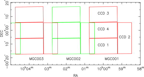
Figure 2: Outline of MGC fields 1, 2 and 3 and the arrangement of the CCDs.

To address the above problems within a single, well-defined dataset we require a survey that is reasonably deep and yet has a large enough solid angle to provide accurate and statistically significant galaxy counts over the crucial normalization range. Furthermore, the survey’s photometry must be accurate and its completeness high, i.e. it must probe to low surface brightnesses. Fig. 1 shows a number of imaging surveys in terms of their sky coverage and magnitude range. Dashed and solid lines indicate photographic and CCD-based surveys, respectively. Typically the faint surveys are CCD-based while the local surveys are photographic (with the notable and recent exception of the SDSS-EDR, Stoughton et al. 2002). While the CCD surveys make significant improvements in surface brightness and magnitude limits their sky coverage is small. It is only very recently that large CCD mosaics such as the Wide Field Camera (WFC, Irwin & Lewis, 2001) and the SDSS instrument (Gunn et al., 1998) have been constructed that now allow a large area of sky to be surveyed within a realistic time frame.

In this paper we present the Millennium Galaxy Catalogue (MGC, Sections 2–5). The MGC represents a new medium-deep, wide-angle galaxy resource, which firmly connects the local and distant universe within a single dataset (cf. Fig 1). In Section 6 we produce the galaxy number counts spanning the range $16\leq B_{\rm MGC}<24$ mag. We then focus on the normalization problem by comparing our counts over the range $16\leq B_{\rm MGC}<20$ mag to the predictions of a number of local luminosity function estimates in Section 7. Our counts provide stringent constraints on the normalization of the luminosity function and hence on the local luminosity density. Our conclusions are given in Section 8.

The 2dFGRS and SDSS will essentially supersede all previous redshift surveys and therefore it is important to verify their photometric accuracy and completeness on as large a scale as possible. We will provide a detailed comparison of the 2dFGRS and SDSS-EDR imaging catalogues with the MGC in a companion paper (Cross et al., 2003).

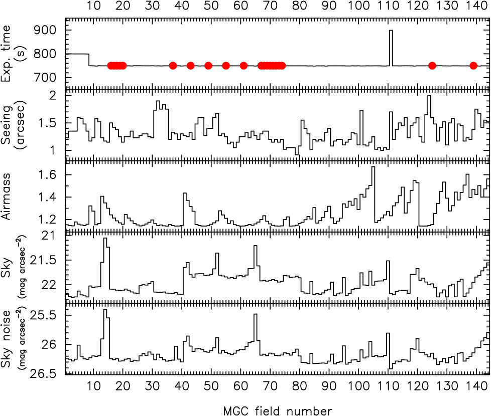
Figure 3: Summary of the data quality across the MGC survey strip. The dots in the uppermost panel indicate the location of the photometric calibration fields. The sky and sky noise parameters were calculated from the measured mode and rms of the background pixel value distribution.

A more long-term aim of the MGC project is to provide structural information on the galaxy population around the crucial normalization point ($16<B<20$ mag). It is ironic that since the advent of the Hubble Space Telescope we have a greater understanding of the morphological mix of galaxies at faint magnitudes than at bright magnitudes. For example, Driver et al. (1998) and Cohen et al. (2003) published morphological galaxy counts spanning the range $21<B_{\rm F450W}<26$ mag, yet no reliable morphological galaxy counts at brighter magnitudes exist. Consequently, no accurate local morphological luminosity functions exist (compare, for example, the conflicting results of Loveday et al. 1992 and Marzke et al. 1998) and the evolution of the different morphological types cannot be accurately constrained. The MGC will enable us to remedy this situation as it allows morphological classification and the extraction of structural parameters to $B_{\rm MGC}=20$ mag.

The data and catalogues presented in this paper are publically available at http://www.roe.ac.uk/$\sim$jol/mgc/.

2 The data

2.1 The Wide Field Camera

All data frames where taken using the Wide Field Camera (WFC). The WFC is mounted at prime focus on the $2.5\,$m Isaac Newton Telescope (INT) situated at La Palma. The WFC is a mosaic of four 4k$\times$2k thinned EEV CCDs with a smaller 2k$\times$2k Loral CCD which is used for auto-guiding. Each of the science CCDs measures $2048\times 4100$ pixels with a pixel scale of $0.333$ arcsec/pixel – this gives a total sky coverage of $0.287$ deg² per pointing. The four science chips are arranged as shown in Fig. 2. Full details of the WFC are provided at http://www.ast.cam.ac.uk/$\sim$wfcsur/technical.html (see also Irwin & Lewis, 2001).

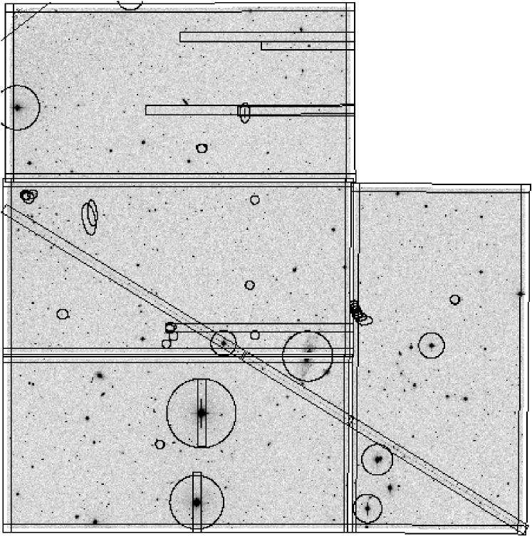
Figure 4: The data of MGC field 36. Overlaid are the exclusion regions due to CCD edges, the vignetted corner of CCD 3 (top), CCD defects, bright stars and galaxies, satellite trails and diffraction spikes (see Section 4.5.2). The exclusion regions reduce the effective area covered by this pointing from $0.260$ deg² to $0.217$ deg².

2.2 The observations

The data constituting the MGC comprise $144$ overlapping fields forming a $35$ arcmin wide equatorial strip from $9^{\rm h}58^{\rm m}28^{\rm s}$ to $14^{\rm h}46^{\rm m}45^{\rm s}$ (J2000). The observations were taken during $4$ observing runs, 1999 March 15–16, 1999 April 16–17, 1999 June 6–13 and 2000 March 26–April 4. Each field was observed for a single $750$ s exposure through a Kitt Peak National Observatory $B$ filter. Field $1$ is centered on RA $=10^{\rm h}00^{\rm m}00^{\rm s}$, Dec $=00\degr 00\arcmin 00\arcsec$ (J2000) and field $144$ is centered on RA $=14^{\rm h}46^{\rm m}00^{\rm s}$, Dec $=00\degr 00\arcmin 00\arcsec$ (J2000). Hence each field is offset from the previous by $30$ arcmin along the equatorial great circle. Fig. 2 shows the survey outline for the first three pointings. Note the substantial overlap between neighbouring fields. The survey region was chosen because it is contained within both the 2dFGRS (Colless et al., 2001) and the SDSS-EDR (Stoughton et al., 2002) regions, thus providing redshifts and colours for the brighter galaxies and allowing a detailed check of the photometry and completeness of these surveys.

All observations were taken during dark or grey time through variable conditions. The seeing ranged from $0.9$ to $2.0$ arcsec with the median seeing at $1.3$ arcsec. The air masses ranged from $1.141$ to $1.672$. Fig. 3 shows a summary of the general observing conditions across the survey.

As much of the data were collected during clear but non-photometric nights it was necessary to dedicate a single pristine photometric night (2000 March 30) to obtaining suitable calibration data at various stages along the survey strip. In total $20$ MGC fields were observed during the photometric night. Of these, six were only $100$ s exposures as they had already been observed previously. These observations were interspersed with $10$ s observations of standard stars spanning a wide range in airmass. The standard stars where taken from the Landolt (1992) standard areas SA98, SA101, SA104 and SA107.

Some science frames were later found to be of too poor a quality to be useful and these were re-observed: the first eight fields were replaced with two $400$ s exposures each and field $111$ is a single $900$ s exposure.

2.3 Data reduction and astrometry

All the preliminary data reduction – flat-fielding, bias correction and astrometric calibration – was done by the Cambridge Astronomy Survey Unit (CASU) and full details of this process are provided by Irwin & Lewis (2001). Briefly, a number of bias frames are collected each night and the median is subtracted from the data. All data (including flat-fields) are corrected for a known non-linearity. A twilight flat-field is taken during evening and morning twilight (when possible) and a median flat-field derived for that particular run is divided into each data frame. After this process an initial astrometric calibration is made to the HST Guide Star Catalogue. Finally the frames are matched to the APM catalogue which itself is calibrated onto the Tycho-2 astrometric system. Fig. 4 shows the final reduced image for one of our pointings, field 36. It illustrates problems with satellite trails, CCD defects, gaps between CCDs, etc.

Figure 5: (a) Median RA differences of doubly detected objects with $17\leq B^{\prime}_{\rm MGC}\leq 21$ mag in overlap regions. The error bars are 68 per cent ranges. (b) Frequency distribution of individual $\Delta$RA values. This distribution has a mean and rms of $-0.016$ and $0.083$ arcsec, respectively. (c) Same as (a) for Dec differences. (d) Same as (b) for $\Delta$Dec. This distribution has a mean and rms of $0.006$ and $0.084$ arcsec.

To assess the final astrometric accuracy we compared the positions of doubly detected objects in regions where neighbouring fields overlap (cf. Fig. 2). The overlap regions are of size $\sim 0.027$ deg² and each contains $\sim 60$ objects in the range $17\leq B^{\prime}_{\rm MGC}\leq 21$ mag, where detections can be easily and confidently matched. Fig. 5 shows the median positional differences for these objects for each overlap region as well as the overall $\Delta$RA and $\Delta$Dec distributions. We find that both of these distributions have an rms of $\pm 0.08$ arcsec. Note, however, that they are slightly but significantly offset from zero which is most likely due to residual radial distortions.

3 Photometric calibration

As mentioned previously, four Landolt (1992) standard star fields were observed at a range of air masses throughout the course of the photometric night. For each observation of each standard star we computed a zero-point

$$ZP_{\rm std}=B+2.5\log f,$$ (1)

where $B$ was taken from Landolt (1992) and $f$ is the flux of the star as measured from the data. We then fitted these zero-points with a double linear function in airmass ($=\sec Z$, where $Z$ is the zenith distance), and colour,

$$ZP_{\rm std}=a+a_{\rm am}\>\sec Z+a_{B-V}(B-V),$$ (2)

where $(B-V)$ is again taken from Landolt (1992). In Fig. 6 we show the data and the fit. The residuals have an rms of $0.02$ mag and show no obvious trend with airmass, colour, $B$ or time of observation. Note, however, that a systematic error of $0.01$ mag was needed to achieve an acceptable fit. From the lower panel of Fig. 6 we can see that for several stars multiple observations of the same star give consistently high or low results. This may indicate that these stars are slightly variable or that the errors on the Landolt (1992) photometry have been underestimated.

Figure 6: Upper panel: colour-corrected zero-points versus airmass. Lower panel: airmass-corrected zero-points versus colour. The solid lines show the best fit (cf. equation 2). The error bars include contributions from photon counting, sky subtraction, read-out noise and the uncertainty in $B$. A further systematic error of $0.01$ mag (added in quadrature) was needed to achieve an acceptable fit.

For each MGC field we then computed a theoretical zero-point $ZP_{\rm th}=a+a_{\rm am}\>\sec Z$, which is expected to be correct only for those fields observed during the photometric night. We extracted objects as described in Section 4 and identified duplicate detections in regions where any two images overlapped. Using only objects with $17\leq B^{\prime}_{\rm MGC}\leq 21$ mag and stellaricity $>0.5$ (cf. Section 4.5) we computed, for each overlap region, the median of the magnitude differences of the double detections, $\langle\Delta B^{\prime}_{\rm MGC}\rangle$, as well as an error on the median, $\sigma_{\langle\Delta B^{\prime}_{\rm MGC}\rangle}$. In Fig. 7(a) we show $\langle\Delta B^{\prime}_{\rm MGC}\rangle$ for all the overlap regions using the initial, theoretical zero-points.

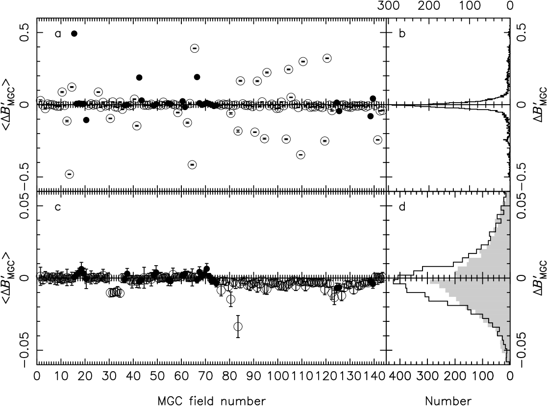
Figure 7: (a) Median magnitude differences of doubly detected objects with $17\leq B^{\prime}_{\rm MGC}\leq 21$ mag and stellaricity $>0.5$ in overlap regions, using initial zero-points. Solid points indicate overlap regions involving at least one photometric observation. The error bars are $68$ per cent ranges divided by the square root of the number of objects (on average $35$). (b) Frequency distribution of all of the individual $\Delta B^{\prime}_{\rm MGC}$ values. (c) Same as (a) using the final zero-points. Note that the scale of the $\langle\Delta B^{\prime}_{\rm MGC}\rangle$-axis is expanded by a factor of $10$ compared with (a). (d) The solid line shows the frequency distribution of the individual $\Delta B^{\prime}_{\rm MGC}$ values using the final zero-points. This distribution has a mean of $-0.002$ mag and an rms of $0.023$ mag. For comparison, the shaded histogram is the same as that shown in (b).

A linear least-squares routine was then used to adjust the zero-points of the non-photometric fields in order to minimize the quantity

$$\chi^{2}=\sum\left(\frac{\langle\Delta B^{\prime}_{\rm MGC}\rangle}{\sigma_{\langle\Delta B^{\prime}_{\rm MGC}\rangle}}\right)^{2},$$ (3)

where the sum goes over all overlap regions. The process of object extraction, matching and zero-point adjustment was then repeated until a stable solution was reached (four iterations).

Since the zero-points of the photometric fields are held fixed at their theoretical values, the above procedure assumes that the observing conditions were perfectly stable throughout the photometric night. One can derive an estimate of the real-life error on the photometric zero-points, $\sigma_{ZP}$, by comparing the scatter of $\langle\Delta B^{\prime}_{\rm MGC}\rangle$ with $\sigma_{\langle\Delta B^{\prime}_{\rm MGC}\rangle}$ for those overlap regions that only involve photometric fields. We found $\sigma_{ZP}=0.005$. Thus we modified the above calibration procedure by including the zero-points of the photometric fields in the parameters to be fitted and adding the additional constraints that they must lie ’close’ to their theoretical values. In other words we now minimize the quantity

$$\chi^{2}=\sum_{\rm all}\left(\frac{\langle\Delta B^{\prime}_{\rm MGC}\rangle}{\sigma_{\langle\Delta B^{\prime}_{\rm MGC}\rangle}}\right)^{2}+\sum_{\rm phot}\left(\frac{ZP-ZP_{\rm th}}{\sigma_{ZP}}\right)^{2},$$ (4)

where the first sum again runs over all overlap regions and the second sum runs over all photometric fields. In Fig. 7(c) we show $\langle\Delta B^{\prime}_{\rm MGC}\rangle$ for all the overlap regions using the final zero-points. Fig. 7(d) shows the histogram of the individual $\Delta B^{\prime}_{\rm MGC}$ values. The width of this distribution indicates an internal photometric accuracy of $0.023$ mag for objects in the range $17\leq B^{\prime}_{\rm MGC}\leq 21$ mag. Due to the paucity of photometric fields beyond MGC field $74$ (cf. top panel of Fig. 3) the absolute calibration in the second half of the survey is less reliable than in the first: up to field $74$ the median of the $\Delta B^{\prime}_{\rm MGC}$ distribution is $3\times 10^{-4}$ mag, which is consistent with zero, but beyond field $74$ it is $-0.004$ mag. This is needed to reconcile the photometric fields $124$ and $139$ with the photometric fields at field numbers $\leq 74$.

Given the above calibration process the relationship between an object’s $B^{\prime}_{\rm MGC}$ magnitude and its Landolt $B$ magnitude is given by:

$$B^{\prime}_{\rm MGC}=B-0.145(B-V),$$ (5)

where the error on the colour term is $\pm 0.002$.

4 Object extraction

Object extraction was performed using Extractor, which is the STARLINK adapted version of SExtractor developed by Bertin & Arnouts (1996).

4.1 Background estimation

SExtractor initially derives a background map by first defining a grid over the image and then passing a median filter (set to a size of $7\times 7$ pixel) over each pixel within the grid cell. The local sky within the grid cell is then taken as the mode or $\sigma$-clipped mean of the pixel distribution within the cell. Finally, a background map is constructed via a bicubic spline interpolation over these points. We opted for the largest possible mesh size ($256\times 256$ pixel) to minimize the smoothing out of any extended low surface brightness features.

4.2 Object detection and deblending

After convolving the image with a filter, SExtractor detects objects as groups of connected pixels above the uniform surface brightness threshold of $\mu_{\rm lim}=26$ mag arcsec^-2. Once an object has been detected SExtractor redetects the object using $30$ different detection thresholds, which are exponentially spaced between the peak flux value of the object and the detection threshold. If at any level the object breaks up into two or more disconnected subcomponents, each containing at least $10$ per cent of the total flux of the object, then the object is deblended. This multithresholding is ideally suited for galaxy extraction because no assumptions concerning the shape of the object are being made (Bertin & Arnouts, 1996).

4.3 Photometry

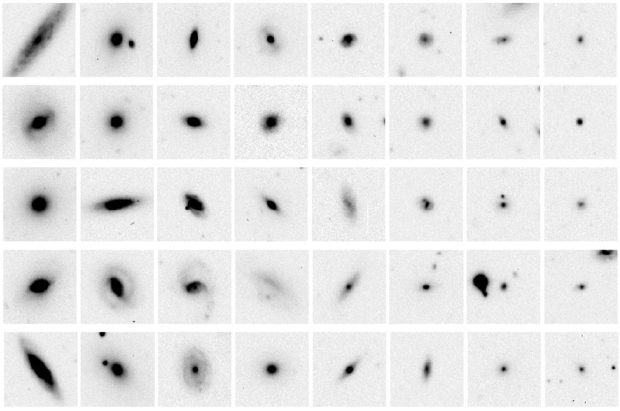
Figure 8: Random examples of the field galaxy population at $B_{\rm MGC}=16.25$ mag (left) in steps of $0.5$ mag to $B_{\rm MGC}=19.75$ mag (right) displayed from $22$ mag arcsec^-2 (black) to $3\sigma$ below the sky (white). The image sizes are $33\times 33$ arcsec².

The photometry was performed using SExtractor with a constant analysis isophote of $26$ mag arcsec^-2 to provide a uniformly processed catalogue. Four of the various types of magnitudes provided by SExtractor are included in the MGC: an isophotal magnitude (ISO), a corrected isophotal magnitude (ISOCOR), an adaptive aperture magnitude (KRON) and a best magnitude (BEST). The ISOCOR magnitude is calculated by correcting the ISO magnitude for the fraction of the flux outside the limiting isophote assuming a Gaussian profile (see Bertin & Arnouts, 1996, and references therein for details). KRON magnitudes (i.e. elliptical apertures of 2.5 Kron radii, Kron 1980) are known to underestimate the fluxes in perfect exponential profiles by $0.04$ mag and in de Vaucouleur profiles by $0.1$ mag. Nevertheless, they have been shown to be the most robust to variations in redshift, bulge-to-disc ratio, isophotal limit and seeing (Cross, 2002). The BEST magnitude is taken to be the KRON magnitude except in crowded regions where the ISOCOR magnitude is used instead. All objects are individually corrected for Galactic extinction using the dust extinction maps provided by Schlegel, Finkbeiner & Davis (1998) and adopting $A_{B_{\rm KPNO}}=4.23$. From now on we refer to the BEST magnitudes before and after extinction correction as $B^{\prime}_{\rm MGC}$ and $B_{\rm MGC}$, respectively. Fig. 8 shows a random selection of galaxies in the range $B_{\rm MGC}=16.25$ to $19.75$ mag.

4.4 Overlap regions

As a result of the substantial overlap regions (cf. Fig. 2) the catalogue contains many duplicate objects. These were used in previous sections to verify the astrometry and to calibrate the photometry. We now remove duplicate detections by imposing RA limits for each field, effectively splitting each overlap region in half. (Note that the RA limits do not apply to objects detected on CCD 3.) For a small number of objects, all lying very close to an RA limit, this procedure did not remove one of the duplicate detections, because the two detections happened to lie on either side of the limit. These cases were fixed by hand.

4.5 Classification and cleaning

At this stage the catalogue contains a total of $1\;070\;374$ objects to $B_{\rm MGC}=24$ mag. The catalogue comprises galaxies, stars and various unwanted objects and artefacts such as satellite trails, CCD defects, cosmic rays, diffraction spikes, asteroids and spurious noise detections. As a starting point for classification we used the stellaricity parameter provided by SExtractor, which is produced for each object by an artificial neural network (ANN) that has been extensively trained to differentiate between stars and galaxies (Bertin & Arnouts, 1996). The input of the ANN consists of nine object parameters (eight isophotal areas and the peak intensity) and the seeing. The output consists of a single number, called stellaricity, which takes a value of $1$ for stars, $0$ for galaxies and intermediate values for more dubious objects. Fig. 9 shows the number of objects as a function of stellaricity and $B^{\prime}_{\rm MGC}$. At $B^{\prime}_{\rm MGC}\la 20$ mag the stellaricity distribution is clearly bimodal with almost all values at the extremes and so star–galaxy separation is trivial. At fainter magnitudes the star–galaxy separation requires more effort. Hence we now define two catalogues: MGC-BRIGHT, which contains all objects with $B_{\rm MGC}<20$ mag, and MGC-FAINT which contains the rest.

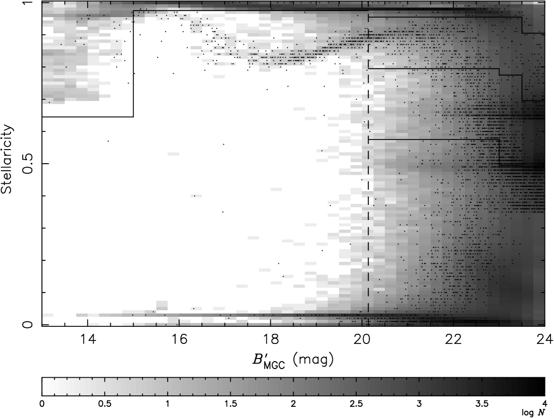
Figure 9: Number of all detected objects as a function of stellaricity and $B^{\prime}_{\rm MGC}$. Dots indicate the positions of objects from the field with the very worst seeing. The vertical dashed line marks the approximate division between MGC-BRIGHT and MGC-FAINT (which was defined in $B_{\rm MGC}$, not $B^{\prime}_{\rm MGC}$). In MGC-BRIGHT, the solid line delineates the division between objects assumed to be stars and those classified by eye. In MGC-FAINT the three solid lines show the star–galaxy separation adopted for the fields with the best, median and worst seeing (see the text for details), where the uppermost line corresponds to the best seeing.

4.5.1 MGC-BRIGHT: $B_{\rm MGC}<20$

For MGC-BRIGHT we adopted the following classification strategy. Brighter than $B^{\prime}_{\rm MGC}=15$ mag we classified all objects with stellaricity $>0.65$ as stars. This low stellaricity cut was used because the objects in the upper left-hand corner of Fig. 9 are, in fact, flooded stars. For the rest of MGC-BRIGHT we classified all objects with stellaricity $\geq 0.98$ as stars. This is a ‘natural’ value to adopt because the stellaricity distribution rises sharply from $0.97$ to $0.98$. All objects so far classified as non-stellar were then inspected visually and classified into one of the following categories: galaxy, star, asteroid, satellite trail, cosmic ray, CCD defect, diffraction spike or spurious noise detection. Incorrectly deblended galaxies were then repaired by hand, but their original catalogue entries were retained and classified as obsolete. Asteroids were verified using images from the SuperCOSMOS Sky Survey (SSS, Hambly et al., 2001). We also inspected all objects with FWHM, semimajor or semiminor axis less than the seeing (these turned out to be primarily cosmic rays and CCD defects). During this process galaxies were also assigned one of three quality classes, $Q$, depending on the level of: (i) contamination by CCD defects, satellite trails, cosmic rays and diffraction spikes; (ii) blending with a similarly bright object; (iii) missing light due to a CCD edge and (iv) failed background estimation due to nearby bright objects. The breakdown of the final MGC-BRIGHT catalogue is shown in Table 1 and is a good indication of the level of contamination in purely automated galaxy catalogues.

Table 1: Breakdown of MGC-BRIGHT ($B_{\rm MGC}<20$ mag).

Description	Number	After cleaning
Galaxies	11866	9913
$\;\;\;(Q^{a}=1,2,3$	11266, 449, 151	9775, 138, 0)
Stars	51284	42365
Asteroids	145	125
Satellite trails	162	0
Cosmic rays	113	62
CCD defects	3027	0
Diffraction spikes	263	0
Noise detections	2023	13
Obsolete	140	116
Total	69023	52594

^aQuality class, where 1 denotes highest quality.

4.5.2 Exclusion regions

Having classified MGC-BRIGHT we now have reasonably good indicators for the positions of CCD defects, satellite trails, very bright objects and diffraction spikes. All of these adversely affect the measurement of parameters of nearby objects. In addition, very bright objects ($B^{\prime}_{\rm MGC}<12.5$ mag) cause a halo of spurious faint detections. Before we continue with the star–galaxy separation in MGC-FAINT it is important to remove as many of these adversely affected and spurious detections as possible. Hence we now define exclusion regions: any objects within these regions will be removed from both MGC-BRIGHT and MGC-FAINT to produce ‘cleaned’ versions of these catalogues.

In particular, we define rectangular or elliptical exclusion regions around CCD edges, the vignetted corner of CCD 3, CCD defects, CCDs 3 and 4 of field 79 (which failed to read out properly), small, unwanted overlaps between CCDs 2 and 3 of a few neighbouring fields, satellite trails, diffraction spikes and objects with $B^{\prime}_{\rm MGC}<12.5$ mag. For most ‘classes’ of exclusion regions we use some simple algorithm to define a first set of exclusion regions from the corresponding class of detections in MGC-BRIGHT. This first set is then improved upon and augmented by hand where necessary. Since the parameters of very bright objects in MGC-BRIGHT are unreliable due to saturation, we have primarily used the SSS to define the last class of exclusion regions.

Fig. 4 shows the exclusion regions for field 36. The exclusion regions reduce the total area of the survey from $37.50$ deg² to $30.84$ deg².

Fields 14, 15 and 65 are of substandard quality because their surface brightness detection limit is considerably brighter than $26$ mag arcsec^-2(cf. bottom panel of Fig. 3). This results in a large number of spurious detections at magnitudes $\ga 23$ mag in these fields. As part of the cleaning process we have therefore removed all objects from these fields from MGC-FAINT (but not from MGC-BRIGHT).

4.5.3 MGC-FAINT: $B_{\rm MGC}\geq 20$

Although MGC-FAINT has been cleaned as described above, it still contains large numbers of cosmic rays, which we now attempt to identify. Cosmic rays are expected to be very small along at least one axis. SExtractor provides object shape parameters in the form of an ‘rms ellipse’. In Fig. 10 we plot all objects from the cleaned versions of MGC-BRIGHT and MGC-FAINT in terms of their flux rms along the minor axis and $B^{\prime}_{\rm MGC}$. We can clearly identify a ‘band’ of objects with $0.7<$ minor axis $<1.0$ pixel (solid lines). From our classification of MGC-BRIGHT and inspection of random samples at fainter magnitudes we found that all objects within this band and $B^{\prime}_{\rm MGC}<22.7$ mag are indeed cosmic rays. Conversely, clearly almost all cosmic rays lie in this band. However, at $B^{\prime}_{\rm MGC}\ga 22.7$ mag the cosmic ray band merges with the general population of objects and a minor axis cut alone is insufficient to select cosmic rays.

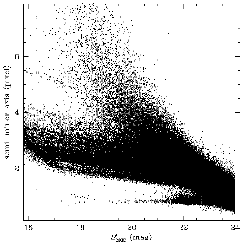
Figure 10: Flux rms along the minor axis versus $B^{\prime}_{\rm MGC}$ for all objects from the cleaned versions of MGC-BRIGHT and MGC-FAINT. Almost all cosmic rays lie in the band delineated by the two solid lines. For $B^{\prime}_{\rm MGC}<22.7$ mag the band is well separated from the general population and hence reliable and complete cosmic ray identification is possible using a minor axis cut alone. At $B^{\prime}_{\rm MGC}\geq 22.7$ mag we apply the additional cut of FWHM $<0.9\times\mbox{\rm seeing}$ to identify cosmic rays but the selection is now incomplete.

SExtractor provides an estimate of the FWHM of the flux profile, assuming a circular Gaussian core. The additional cut of FWHM $<0.9\times\mbox{\rm seeing}$ is successful in identifying large numbers of cosmic rays at $B^{\prime}_{\rm MGC}\geq 22.7$ mag. The remaining unidentified cosmic rays are those with a large angle of incidence which leave a faint ‘trail’ on the images. Unfortunately, given the parameters available from SExtractor this class of cosmic rays is genuinely indistinguishable from real objects, and hence the identification of cosmic rays at $B^{\prime}_{\rm MGC}\geq 22.7$ mag must remain incomplete. In Section 6.4 we estimate this incompleteness to be $<20$ per cent and correct the galaxy number counts accordingly.

All objects in the cleaned version of MGC-FAINT not identified as cosmic rays by the above procedure are assumed to be either stars or galaxies. As we have noted above, for $B^{\prime}_{\rm MGC}\ga 20$ mag star–galaxy separation becomes increasingly difficult. However, Kümmel & Wagner (2001) showed that the slope of the star counts remains constant to $B=22.75$ mag, in agreement with Galaxy model predictions (Bahcall & Soneira, 1980; Bahcall, 1986). Hence one can produce statistical galaxy number counts without explicitly classifying individual objects by simply subtracting the expected stellar counts (determined by extrapolation from the bright end) from the measured total counts.

Nevertheless, a variety of applications do require classifications for individual objects and so we adopt the following scheme. The idea is to find a stellaricity value, $s_{\rm c}$, such that the objects with stellaricity $>s_{\rm c}$ reproduce the numbers of stars expected by extrapolating the stellar counts measured in the range $17\leq B^{\prime}_{\rm MGC}<20$ mag. However, the ability of SExtractor to distinguish between stars and galaxies depends both on magnitude and the seeing. Moving to fainter magnitudes or worse seeing both have the effect of redistributing stars from the high end of the stellaricity distribution towards intermediate values. Therefore, we must determine $s_{\rm c}$ as a function of $B^{\prime}_{\rm MGC}$ for each MGC field individually.

Since for a given field $s_{\rm c}(B^{\prime}_{\rm MGC})$ should be monotonic and since the exact placement of $s_{\rm c}$ is most crucial at the faint end, we have adopted the following strategy: for each field we first adjust $s_{\rm c}$ in the field’s faintest three bins (determined by the field’s completeness limit, see Section 4.6) to give star count values closest to the extrapolated bright star count fit (in a $\chi^{2}$ sense), while requiring $s_{\rm c}(B^{\prime}_{\rm MGC})$ to be monotonic. In all remaining bins with $B^{\prime}_{\rm MGC}\geq 20$ mag we set $s_{\rm c}$ to the highest $s_{\rm c}$ value so far obtained. The bright star count fit is derived locally for each field from the stellar counts in the range $17\leq B^{\prime}_{\rm MGC}<20$ mag as measured from the five fields centered on the field under consideration (to improve the reliability of the fit). In Fig. 9 we show the resulting $s_{\rm c}$ curves for the fields with the best, median and worst seeing. As expected we found that the value of $s_{\rm c}$ correlates strongly with seeing.

The error on the galaxy number counts introduced by the uncertainty in the exact placement of $s_{\rm c}$ is discussed in Section 6.1.

4.6 Faint completeness limits

In order to estimate the faint completeness limit for each field we used the artdata package of IRAF to add $100$ equally bright point sources at random positions (but avoiding exclusion regions) to each CCD of each field. We then re-extracted object lists to determine whether the simulated objects were recovered. Detections that were judged to be due to a blend of a simulated object and a real object of similar or greater brightness were not counted as recovered. This process was repeated for a total of $14$ input magnitudes in the range $22\leq B^{\prime}_{\rm MGC}<26$ mag. For each field we then fitted a three-parameter completeness function to the fraction of recovered objects as a function of magnitude (cf. Kümmel & Wagner, 2001):

$$c(B^{\prime}_{\rm MGC})=\left[\exp\left(\frac{B^{\prime}_{\rm MGC}-B^{\prime}_{50}}{\beta}\right)+\frac{1}{c_{\rm b}}\right]^{-1},$$ (6)

where $c_{\rm b}$ is the completeness at bright magnitudes and $B^{\prime}_{50}$ is the magnitude at which the completeness reaches $c(B^{\prime}_{50})=c_{\rm b}(c_{\rm b}+1)^{-1}\approx 0.5$. In general $c_{\rm b}\neq 1$ because some small fraction of objects will always be covered up by brighter objects and thus go undetected.

We find that $c_{\rm b}$ is weakly correlated with seeing, varying from 0.995 to 0.965 with a mean value of $\overline{c_{\rm b}}=0.983$. $B^{\prime}_{50}$ is quite strongly correlated with seeing while $\beta$ correlates with the sky noise ($\overline{\beta}=0.22$).

For each field we now define a magnitude limit by $c(B^{\prime}_{\rm lim})=fc_{\rm b}$, where we take $f=0.97$ so that the mean completeness at the magnitude limit is $\overline{c(B^{\prime}_{\rm lim})}=f\overline{c_{\rm b}}>0.95$. Finally, for a given field we define a dust-corrected magnitude limit, $B_{\rm lim}$, as the brightest $B_{\rm MGC}$ of all objects with $B^{\prime}_{\rm MGC}\geq B^{\prime}_{\rm lim}$ in that field. In the following we will only use objects with $B_{\rm MGC}<B_{\rm lim}$ and we will not attempt to use fainter objects in combination with incompleteness corrections. Hence, when constructing the number counts we will only use a given field for a given magnitude bin if the field covers the entire bin (of size $\Delta B_{\rm MGC}=0.5$ mag). Thus we are effectively rounding the magnitude limit of the field downwards to the nearest multiple of $0.5$. This leaves $124$ fields in the $B_{\rm MGC}=23.25$ mag bin and $14$ fields in the faintest bin at $B_{\rm MGC}=23.75$ mag.

4.7 Object distribution in RA

Fig. 11 shows how the MGC-BRIGHT (upper panel) and MGC-FAINT (lower panel) galaxies are distributed along the MGC survey strip. The vertical dashed lines indicate the positions of known $z<1$ galaxy clusters. It is encouraging to note that on the whole they coincide with peaks in the galaxy numbers.

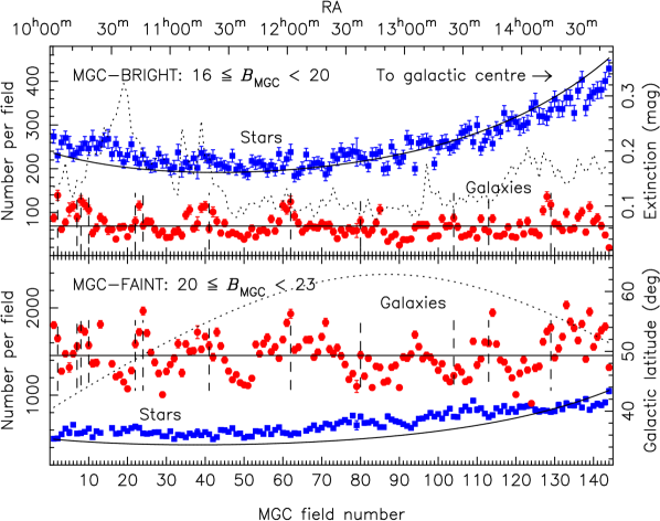
Figure 11: The distribution of galaxies and stars in MGC-BRIGHT (top panel) and MGC-FAINT (bottom panel) as a function of MGC field number or RA (indicated along top). The dashed vertical lines indicate the positions of $z<1$ galaxy clusters found in the literature. The galaxies show a uniform distribution whereas the stars show a clear rise towards the Galactic Centre. The solid horizontal lines indicate the mean number of bright and faint galaxies per field. The curved solid lines represent the star counts predicted by the standard Galaxy model of Bahcall & Soneira (1980) and Bahcall (1986). All numbers have been scaled to a constant area of $0.215$ deg² per field. The dotted lines and right axes indicate how the extinction and galactic latitude vary across the survey.

We also show how the numbers of stars vary across the survey strip and how they compare to predictions of the standard Galaxy model of Bahcall & Soneira (1980) and Bahcall (1986). The basic shape of the counts and the model agree in that there is a clear rise towards the galactic bulge. However, there appear to be significant differences. The model systematically under-predicts the faint counts and there are also discrepancies with the bright counts at low galactic latitudes. Similar trends are apparent in the stellar $r^{*}$ counts of Yasuda et al. (2001). We will address this issue in more detail in a future paper (Lemon et al., 2003).

5 Selection limits

One of the primary aims of the MGC was to define a sample of galaxies with well-defined selection criteria, hence the use of a constant detection isophote. Fig. 12 shows the distribution of galaxies in the apparent magnitude – apparent effective surface brightness plane for MGC-BRIGHT. The apparent effective surface brightness was simply calculated as

$$\mu_{\rm eff}=B_{\rm MGC}+2.5\log(2\pi r_{1/2}^{2}),$$ (7)

where $r_{1/2}$ is the semimajor axis of the ellipse containing half the total flux (in arcsec) which was measured directly from the data.

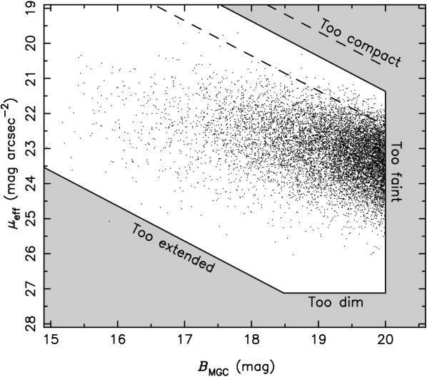
Figure 12: The apparent bivariate brightness distribution of MGC-BRIGHT galaxies. The shaded regions show the selection boundaries determined by the median seeing (upper diagonal line), the magnitude limit (vertical line), the surface brightness detection limit (horizontal line) and the mesh size employed during the background estimation (lower diagonal line, see the text for details). The two dashed lines are the selection limits for the fields with the worst (lower) and the best (upper) seeing.

The solid lines delineating the shaded regions in Fig. 12 show the selection boundaries. The three principal selection limits are the median seeing limit of $1.3$ arcsec, the central surface brightness detection limit of $\mu_{\rm lim}=26$ mag arcsec^-2 (equivalent to an effective surface brightness limit of $27.12$ mag arcsec^-2, assuming an exponential profile) and the imposed magnitude limit of $B_{\rm MGC}=20$ mag. Note that this cut was set by the magnitude limit at which star–galaxy separation is reliable.

A fourth selection limit is implied by the method of background estimation described in Section 4.1. Any objects covering a substantial fraction of a cell of the grid used to estimate the background will produce an erroneously high background measurement and hence may be missed. We estimate that objects with an isophotal area of $\sim 25$ per cent of a grid cell will be affected. We have used a mesh size of $256\times 256$ pixel ($85.2\times 85.2$ arcsec). Assuming $r_{\rm iso}\approx 2r_{1/2}$ this represents an upper size limit in terms of half-light radius of $64$ pixel ($21.3$ arcsec). This line is shown as the lower diagonal selection limit in Fig. 12.

Outside the selection boundaries galaxies cannot, theoretically, be detected although noise may scatter a few objects across these boundaries. Galaxies with parameters inside the boundaries should be detectable. The galaxy population follows a well-defined distribution, which does not reach to the high and low surface brightness selection boundaries, demonstrating the robustness of MGC-BRIGHT with respect to surface brightness selection effects. The distribution in surface brightness of the observed population is far too narrow to be explained by visibility theory (see Cross & Driver, 2002) and one must conclude that luminous low surface brightness galaxies are indeed rare as suggested by Driver (1999), Cross et al. (2001) and Blanton et al. (2001).

6 Number counts

6.1 Errors

Before we present the final galaxy counts we will estimate realistic errors for the counts. In addition to Poisson noise they should also contain a contribution from large-scale structure (LSS), which will also induce correlations between different bins. If galaxies have an angular correlation function $w(\theta)=A_{w}\theta^{1-\gamma}$ then the error on the counts in a given bin, $\sigma_{N}$, is given by (Peebles, 1980)

$$\sigma_{N}(B_{\rm MGC})=A^{-1}\sqrt{{\cal N}+{\cal N}^{2}A_{w}C},$$ (8)

where ${\cal N}$ is the number of galaxies in the bin, $A$ is the survey area and $C$ is the integral constraint given by a double integral over the survey area:

$$C=A^{-2}\int\!\!\!\int\theta^{1-\gamma}{\rm d}\omega_{1}{\rm d}\omega_{2},$$ (9)

where we will use the SDSS-EDR results on $w(\theta)$ of Connolly et al. (2002), who found $1-\gamma\approx-0.7$ and measured $\log A_{w}$ as a function of $r^{*}$. We translate these measurements to $B_{\rm MGC}$ (using equation 5, the colour equations of Fukugita et al. 1996 and the mean galaxy colours of Yasuda et al. 2001) and extrapolate where necessary. The resulting error estimates are shown as crosses in Fig. 13. In fact, we follow the detailed description of Yasuda et al. (2001) to calculate the full covariance matrix for the counts, which will be needed in Section 7.3.

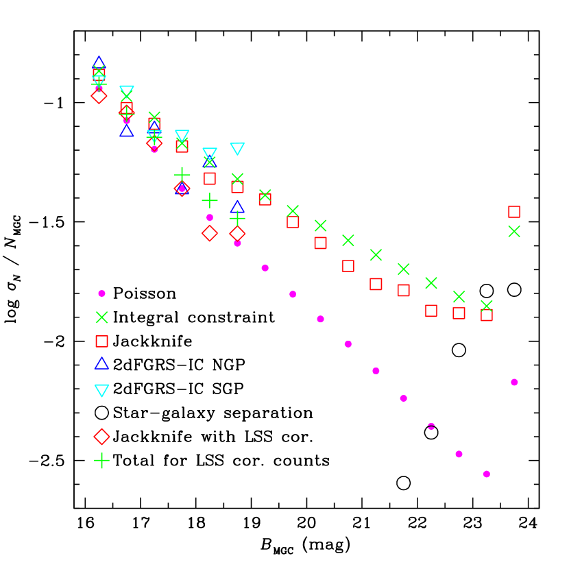
Figure 13: Various estimates of the error on the MGC galaxy number counts, $\sigma_{N}$, scaled by the number counts, $N_{\rm MGC}$, as indicated and described in the text. The last two sets refer to the MGC-2dFGRS counts discussed in Section 6.2. The crosses and ‘+’ symbols show the final errors listed in Table 2.

We have also estimated the covariance matrix using the jackknife method (Efron, 1982). This was implemented by excluding each field from the dataset in turn and measuring the counts from the remaining data. The covariance of these $N_{\rm F}$ measurements is then multiplied by $(N_{\rm F}-1)^{2}N_{\rm F}^{-1}$, where $N_{\rm F}$ is the number of fields used for a given pair of bins. The result agrees well with the integral constraint estimate above and we show the resulting errors as open squares in Fig. 13.

Finally, we have estimated the errors using the 2dFGRS imaging catalogue (2dFGRS-IC). We have divided the North and South Galactic Pole regions (NGP and SGP) into $21$ and $32$ subregions, respectively, each of similar size and shape as the MGC survey region. We converted the 2dFGRS-IC magnitudes to the $B_{\rm MGC}$ filter system using $B_{\rm MGC}=b_{\rm J}+0.074$ (which includes a known offset of $0.056$ mag; cf. equation 7.1). We then measured the counts in each independent subregion and plot the rms of these sets separately for the NGP and SGP as triangles in Fig. 13. This is only possible at $B_{\rm MGC}<19$ mag due to the magnitude limit of the 2dFGRS-IC (Colless et al., 2001).

We note that all of the above error estimates are in reasonably good agreement and lie well above the Poisson errors (solid dots). Henceforth we will adopt the integral constraint estimates.

In Fig. 13 we also plot as open circles an estimate of the uncertainty introduced by the star–galaxy separation in MGC-FAINT. We have varied the method of determining $s_{\rm c}$ (cf. Section 4.5.3) in numerous ways but we only found a significant change in the number counts by systematically increasing (or decreasing) $s_{\rm c}$ in all fields. The error shown in Fig. 13 is the difference in the counts arising from a global change of $s_{\rm c}$ by $0.01$. We note that such a change produces a severe mismatch between the measured faint star counts and those expected from extrapolating the bright counts. Hence the derived error is probably an overestimate. In any case, it is well below the jackknife errors in all but one bin and we therefore do not consider it any further.

6.2 Correcting for large-scale structure

Since the MGC survey region is contained within the 2dFGRS-IC NGP region the question arises as to whether the photometric accuracy and high completeness of the former can be combined with the large area of the latter to derive number counts less affected by LSS and hence of higher accuracy. The idea is to view the ratio of $N_{\mbox{\scriptsize IC-MGC}}$, the 2dFGRS-IC counts within the MGC region, to $N_{\rm IC}$, the counts from a much larger 2dFGRS-IC sample, as an LSS correction factor, which can be applied to the MGC counts to give LSS-corrected counts:

$$N_{\rm MGC}^{\rm cor}=\frac{N_{\rm IC}}{N_{\mbox{\scriptsize IC-MGC}}}\;N_{\rm MGC}.$$ (10)

Equivalently, one can view $N_{\rm MGC}/N_{\mbox{\scriptsize IC-MGC}}$ as a factor being applied to $N_{\rm IC}$, which corrects for incompleteness, stellar contamination, bad deblending, etc. in the 2dFGRS-IC. Hence we will refer to $N_{\rm MGC}^{\rm cor}$ as the MGC-2dFGRS counts.

Figure 14: The top panel shows various galaxy number count estimates derived from the 2dFGRS-IC as indicated: full sample, NGP only ($740.3$ deg²), SGP only ($1094.7$ deg²), in the MGC survey region, in $21$ independent NGP subregions, each of a size and shape similar to the MGC region. We also plot the counts predicted by the 2dFGRS luminosity function (cf. Section 7.1). The error bars on the NGP and SGP counts were calculated using the integral constraint method. The middle panel shows the LSS correction factors using the full, NGP only and predicted counts (same symbols as in top panel). The bottom panel shows the uncorrected MGC counts (crosses) as well as the MGC-2dFGRS counts using the correction factors of the middle panel (same symbols). Several sets of counts in the top and bottom panels have been offset by $\pm 0.1$ mag for clarity.

Fig. 14 illustrates the LSS correction procedure. In the top panel we plot $N_{\mbox{\scriptsize IC-MGC}}$ as crosses along with four sets of large-area counts for possible use as $N_{\rm IC}$ (open symbols). The middle panel shows the LSS correction factors using the full, NGP and predicted counts (same symbols as in top panel), and the bottom panel shows both the uncorrected MGC counts (crosses) and the MGC-2dFGRS counts using the above correction factors.

For this correction procedure to be valid we require only that the properties of the 2dFGRS-IC (photometry, incompleteness, etc.) are homogeneous over the region used to derive $N_{\rm IC}$ and the MGC region. However, in the top panel of Fig. 14 the SGP appears very significantly underdense in comparison to the NGP. Indeed, Norberg et al. (2002) found a $7$ per cent difference in the numbers of NGP and SGP galaxies to $b_{\rm J}=19.2$ mag but concluded that this was ‘reasonably common’ in their mock galaxy catalogues derived from $N$-body simulations. Here we take a more cautious approach and admit the possibility of a systematic difference between the NGP and SGP, possibly a photometric offset. Indeed, we have found an offset of $0.056$ mag between the MGC and the 2dFGRS-IC NGP. Here and in the previous section we have included this offset in the conversion from $b_{\rm J}$ to $B_{\rm MGC}$. Applying this offset only to the NGP, but not the SGP, makes the difference worse.

Since we require homogeneity for the LSS correction to work we choose not to use any SGP data in $N_{\rm IC}$. On the other hand, the NGP seems reasonably homogeneous. In the top panel of Fig. 14 we plot as solid dots the counts from 21 independent, MGC-shaped subregions of the NGP. We can see that the MGC region is typical and from Fig. 13 we have already seen that the variance among these subregions agrees well with that expected. Hence we will use the NGP counts as $N_{\rm IC}$.

What are the error properties of the MGC-2dFGRS counts? Defining $f_{\rm inc}=N_{\rm MGC}/N_{\mbox{\scriptsize IC-MGC}}$ we have

$$\sigma_{N_{\rm MGC}^{\rm cor}}^{2}=\sigma_{f_{\rm inc}}^{2}N_{\rm IC}^{2}+f_{\rm inc}^{2}\sigma_{N_{\rm IC}}^{2}+2\rho f_{\rm inc}N_{\rm IC}\sigma_{f_{\rm inc}}\sigma_{N_{\rm IC}},$$ (11)

where $\rho$ is the correlation coefficient between $f_{\rm inc}$ and $N_{\rm IC}$. A large value of $f_{\rm inc}$ indicates that many galaxies in the MGC region are missed by the 2dFGRS-IC. However, this will be true everywhere if the properties of the 2dFGRS-IC are homogeneous. Hence $N_{\rm IC}$ will be low if $f_{\rm inc}$ is large and vice versa, i.e. $\rho$ must be negative and we will err on the side of caution by neglecting the last term. The first term can be estimated using the jackknife method. For each ‘subsample’ (generated by excluding one field) we calculate $N_{\rm MGC}^{\rm cor}$. Since $N_{\rm IC}$ does not vary from subsample to subsample the resulting error estimate is just the first term above, which we plot as open diamonds in Fig. 13. The estimate agrees very well with the Poisson errors of $N_{\rm MGC}$ (or $N_{\rm MGC}^{\rm cor}$). Since $f_{\rm inc}\approx 1$ we will use

$$\sigma_{N_{\rm MGC}^{\rm cor}}^{2}=\frac{N_{\rm MGC}}{A}+\sigma_{N_{\rm IC}}^{2},$$ (12)

where we estimate the second term as well as the rest of the covariance matrix using the integral constraint method. The result is shown as ‘+’ symbols in Fig. 13. We find that the errors of the MGC-2dFGRS counts are smaller by $12$–$32$ per cent than the errors of the counts obtained from the MGC alone.

6.3 Correcting for asteroids

As a result of their extended morphology asteroids will be classified as galaxies in MGC-FAINT. Recently, Ivezić et al. (2001) performed accurate measurements of the shape of the number counts of both C- and S-type asteroids for $B_{\rm MGC}\la 22.5$ mag from SDSS-CD. Here we adopt their model, normalized to the number of visually identified asteroids in MGC-BRIGHT, and subtract the model asteroid counts from the galaxy counts (cf. Fig. 16).

6.4 Correcting for cosmic ray incompleteness

In Section 4.5.3 we noted that the identification of cosmic rays is incomplete for $B^{\prime}_{\rm MGC}\geq 22.7$ mag. Here we will estimate the size of the incompleteness and correct the galaxy number counts accordingly.

Figure 15: Upper panel: the dots show the number counts of all objects in the cosmic ray band delineated by the two solid lines in Fig. 10. The squares show the number counts of objects selected by applying the additional cut FWHM $<0.9\times\mbox{\rm seeing}$. Lower panel: the ratio of the above counts appears to remain constant to $B^{\prime}_{\rm MGC}=22.7$ mag (dotted line), where real objects begin to contaminate the counts from the cosmic ray band. The incompleteness of cosmic rays selected by the additional FWHM cut is found to be $18.1$ per cent and is indicated by the solid horizontal line.

In the upper panel of Fig. 15 we plot as solid dots the number counts of all objects in the cosmic ray band delineated by the solid lines in Fig. 10. For $B^{\prime}_{\rm MGC}<22.7$ mag these represent the complete cosmic ray counts but beyond $22.7$ mag they are ‘contaminated’ by real objects. At $21\leq B^{\prime}_{\rm MGC}<22$ mag the counts are very steep and would exceed the galaxy counts by $B^{\prime}_{\rm MGC}\approx 23$ mag if they did not flatten out. In the range $22\leq B^{\prime}_{\rm MGC}<22.5$ mag the counts indeed show some flattening. This behaviour makes it impossible to reliably extrapolate the cosmic ray counts to fainter magnitudes (as we do for the stars and asteroids).

We plot as solid squares the number counts of those objects that lie in the cosmic ray band and have FWHM $<0.9\times\mbox{\rm seeing}$, which we use as cosmic ray identification criteria at $B^{\prime}_{\rm MGC}\geq 22.7$ mag. By taking the ratio of the two sets of counts in the lower panel of Fig. 15 we find that for $B^{\prime}_{\rm MGC}<22.7$ mag $81.9$ per cent of all objects within the cosmic ray band also have FWHM $<0.9\times\mbox{\rm seeing}$ and that this ratio remains constant to within the errors. We now assume that this ratio remains constant at $B^{\prime}_{\rm MGC}\geq 22.7$ mag and correct the cosmic ray number counts in the range $22.5\leq B_{\rm MGC}<24$ mag by applying a factor of $1.22$. The difference between the corrected and uncorrected counts is then subtracted from the galaxy counts.

6.5 Number counts

We present the MGC number counts in Fig. 16 and list the galaxy counts in Table 2. Note that the correction for LSS (which affects the counts only in the range $16\leq B_{\rm MGC}<19$ mag) is relatively large at $B_{\rm MGC}=17.25$ mag (17 per cent) but $\la 4$ per cent in all other bins (cf. middle panel of Fig. 13). At $\la 1.1$ and $\sim 1.4$ per cent the asteroid and cosmic ray incompleteness corrections (which affect the counts only at $B_{\rm MGC}\geq 20$ and $B^{\prime}_{\rm MGC}\geq 22.7$ mag, respectively) are smaller still.

Figure 16: MGC number counts as indicated. The open circles refer to the galaxy counts corrected for LSS ($B_{\rm MGC}<19$ mag), asteroids ($B_{\rm MGC}\geq 20$ mag) and cosmic ray incompleteness ($B^{\prime}_{\rm MGC}\geq 22.7$ mag). The open triangles show the cosmic ray counts corrected for incompleteness at $B^{\prime}_{\rm MGC}\geq 22.7$ mag. The solid line shows the adopted Ivezić et al. (2001) model for the asteroid counts, which we extrapolate beyond the faint limit probed by these authors (dashed line).

Table 2: MGC galaxy number counts.

$B_{\rm MGC}$	${\cal N}^{a}$	Area	$N_{\rm MGC}^{b}$	$\sigma_{N}^{c}$	${N_{\rm MGC}^{\rm cor}}^{d}$	$\sigma_{N^{\rm cor}}$
(mag)		(deg2)
16.25	78	30.84	2.53	0.34	2.44	0.30
16.75	143	30.84	4.64	0.49	4.90	0.41
17.25	242	30.84	7.85	0.68	8.67	0.56
17.75	523	30.84	17.0	1.1	16.77	0.84
18.25	925	30.84	30.0	1.7	28.7	1.2
18.75	1497	30.84	48.5	2.3	49.2	1.6
19.25	2433	30.84	78.9	3.2	78.9	3.2
19.75	4016	30.84	130.2	4.6	130.2	4.6
20.25	6495	30.25	214.7	6.5	212.4	6.5
20.75	10568	30.25	349.4	9.2	346.1	9.2
21.25	17727	30.25	586	13	581	13
21.75	30074	30.25	994	20	988	20
22.25	51663	30.25	1708	30	1698	30
22.75	88353	30.25	2921	45	2869	45
23.25	129936	26.71	4865	68	4782	68
23.75	22068	2.91	7581	219	7451	219

^aNumber of galaxies in the MGC in units of ($0.5$ mag)^-1.
^bNumber counts in units of ($0.5$ mag)^-1 deg^-2.
^cIntegral constraint estimate of Section 6.1.
^dNumber counts corrected for LSS ($16\leq B_{\rm MGC}<19$ mag), asteroids ($B_{\rm MGC}\geq 20$ mag) and cosmic ray incompleteness ($B^{\prime}_{\rm MGC}\geq 22.7$ mag).

Fig. 17 compares the MGC galaxy number counts to those of previous surveys. In the range $16\leq B_{\rm MGC}<24$ mag our counts lie among the montage of previous publications and provide a fully consistent, uniform, well-selected and complete sample spanning eight magnitudes. The data thus represent a significant connection between the local photographic surveys ($B\la 20$ mag) and the deep pencil beam CCD surveys ($B\ga 22$ mag). At bright magnitudes our counts are consistently higher than the original APM counts (Maddox et al., 1990b) and suggest that the steep rise of the APM counts is an artefact. We note that the 2dFGRS-IC is a substantially revised version of the APM catalogue and shows a less pronounced rise. Although some local effect is still evident (cf. Fig. 18) there is no more need for strong local evolution of the luminous galaxy population as originally put forward by Maddox et al. (1990b).

Fig. 18 shows a close-up comparison of the MGC-BRIGHT, SDSS-EDR, 2dFGRS-IC NGP and Gardner et al. (1996) counts, where we have normalized the counts by an arbitrary linear model in order to make any differences more easily discernible.

We have used the SDSS-EDR $g^{*}$ counts of the Northern stripe of Yasuda et al. (2001) and converted to $B_{\rm MGC}$ using equation (5), the colour equation of Fukugita et al. (1996) and the galaxy colours as a function magnitude of Yasuda et al. (2001). Alternatively, we could have used Yasuda et al.’s $B$ counts which were derived using individual galaxy colours rather than a mean colour for a given magnitude. However, the colour equation used by Yasuda et al. is inconsistent with that of Fukugita et al. (1996). We prefer the latter over the former because it was used in a direct comparison of SDSS-EDR and MGC magnitudes, which showed essentially no overall zero-point offset between the two surveys (Cross et al., 2003). It was also used in Norberg et al.’s comparison of the 2dFGRS and SDSS-EDR photometry, which also showed only a small difference of $\Delta m($2dFGRS$-$SDSS-EDR$)=0.058$ mag.

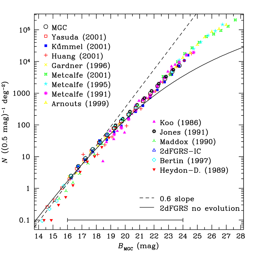
Figure 17: The galaxy number counts derived from the MGC as compared with the number counts of various other authors. The various counts were converted onto the $B_{\rm MGC}$ system assuming $\overline{(B-V)}=0.94$ (Norberg et al., 2002). The 2dFGRS no-evolution model counts are calculated from the luminosity function parameters given in Table 3 (cf. Section 7.1). Also shown is the 0.6 ‘Euclidean’ slope.

Figure 18: A close-up comparison over the important normalization range $16\leq B_{\rm MGC}<20$ mag of the MGC number counts with three other datasets as indicated. The MGC error bars are the integral constraint estimates (cf. Sections 6.1, 6.2 and Table 2). The SDSS-EDR and 2dFGRS-IC errors are also integral constraint estimates, whereas the Gardner et al. (1996) errors are those published.

Fig. 18 shows that the MGC and SDSS-EDR counts are in reasonably good agreement. In particular, both show a characteristic change of slope near $B_{\rm MGC}=18$ mag. However, the SDSS-EDR counts are higher than the MGC counts in the range $18\leq B_{\rm MGC}<21$ mag by $4$–$7$ per cent. Given that Cross et al. (2003) found no offset between the MGC and SDSS-EDR photometries this difference cannot be explained photometrically. However, the error bars in Fig. 18, which include an LSS component, indicate that the difference is not significant and may well be caused by LSS.

Nevertheless, we point out that the definition of a galaxy varies among different SDSS publications. The central tool of the SDSS-EDR star–galaxy separation is the difference between the point spread function (PSF) and model magnitudes, $c$, of an object. The standard SDSS-EDR procedure is to classify an object as a galaxy if it satisfies the condition $c>0.145$ (Stoughton et al., 2002). Yasuda et al. use a slight variant in that they require $c>0.145$ in two of the three bands $g^{*},r^{*}$ and $i^{*}$. However, Blanton et al. (2001) use a cut-off value of $0.242$ in the $r^{*}$ band. Strauss et al. (2002) even use a value of $0.3$ in the SDSS spectroscopic target selection in addition to a surface brightness cut and further selection based on photometric flags. They find that at the bright magnitudes of the spectroscopic sample ($r^{*}\la 17.8$ mag) only $10$ per cent of all objects with $0.15<c<0.3$ are actually galaxies (see also their fig. 7) and they conclude that their sample completeness is $>99$ per cent.

Hence contamination by misclassified objects may in part be responsible for the observed difference between the MGC and SDSS-EDR counts. Indeed, the object-by-object comparison of Cross et al. (2003, in the range $16\leq B_{\rm MGC}<20$ mag) found the SDSS-EDR galaxy sample contaminated by stars and artefacts at the $\sim 1$ per cent level.

Comparing the uncorrected MGC and 2dFGRS-IC counts we note that the latter are generally lower by $5$–$10$ per cent at $B_{\rm MGC}<18.5$ mag, although the difference is again only marginally significant. We note that in the transformation from $b_{\rm J}$ to $B_{\rm MGC}$ magnitudes we have used the Blair & Gilmore (1982) colour term of $0.28$ (cf. equation 7.1) and a global mean galaxy colour of $\overline{(B-V)}=0.94$ (Norberg et al., 2002). Using instead a colour term of $0.35$, as favoured by Metcalfe et al. (1995), or a larger mean galaxy colour, which may be reasonable for the fainter galaxies, both exacerbate the difference. In any case, the small photometric offset between the MGC and 2dFGRS-IC photometries has already been taken into account and hence the difference cannot be explained photometrically. However, a difference of this magnitude is easily explained by the incompleteness and stellar contamination in the 2dFGRS-IC, which were found to be $\sim 9$, and $\sim 6$ per cent, respectively (Pimbblet et al., 2001; Norberg et al., 2002; Cross et al., 2003).

As far as we are aware, apart from the SDSS-EDR and the MGC the largest CCD survey from which number count data have been published is the $8.5$ deg² survey of Gardner et al. (1996). Although generally lower than the MGC counts by $\sim 10$ per cent the error bars indicate that the difference may well be due to LSS.

7 Refining the field galaxy luminosity function

The field galaxy luminosity function (LF) has been measured by many surveys but, as pointed out by Cross et al. (2001), their results – and in particular their derived normalizations – are inconsistent with each other (cf. also Fig. 19a). Depending on which of the many LFs one selects, one will predict markedly different galaxy counts, even locally (see Fig. 19b). In the following section we use the local galaxy counts derived in Section 6 to assess which LFs predict counts consistent with the data and to provide stringent constraints on the LF normalization.

7.1 Modeling the number counts

Table 3: Parameters of published luminosity functions (cf. Fig. 19) and their revised normalizations and luminosity densities. For each LF we also list the probability that its number count predictions fit the data before and after the adjustment of $\phi^{*}$ (eight and seven degrees of freedom, respectively).

LF	Filter conversion	$\bar{z}$	$M^{*}_{B_{\rm MGC}}-5\log h$		$\alpha$		$\phi^{*}$		$P(\geq\chi^{2}_{\rm min})$	$\phi^{*}_{\rm MGC}\mbox{}^{a}$		$P(\geq\chi^{2}_{\rm min})$	$j_{b_{\rm J}}$
	$B_{\rm MGC}=$		(mag)				($10^{-2}h^{3}$ Mpc-3)			($10^{-2}h^{3}$ Mpc-3)			($10^{8}\;h\;L_{\odot}$ Mpc-3)
2dFGRS	$b_{\rm 2dFGRS}+0.07$	$0.1$	$-19.59$ $\pm$	$0.008^{b}$	$-1.21$ $\pm$	$0.01$	$1.61$ $\pm$	$0.06$	$0.18$	$1.69$ $\pm$	$0.04\pm 0.03\pm 0.03$	$0.44$	$2.03$ $\pm$	$0.05$
SDSS-CD	$g^{*}+0.40$	$0.1$	$-19.64$ $\pm$	$0.04$	$-1.26$ $\pm$	$0.05$	$2.06$ $\pm$	$0.23$	$0$	$1.56$ $\pm$	$0.04\pm 0.11\pm 0.03$	$0.40$	$2.06$ $\pm$	$0.11$
ESP	$b_{\rm J}+0.13$	$0.1$	$-19.59$ $\pm$	$0.08$	$-1.22$ $\pm$	$0.07$	$1.65$ $\pm$	$0.3$	$0.45$	$1.68$ $\pm$	$0.04\pm 0.20\pm 0.03$	$0.42$	$2.04$ $\pm$	$0.12$
CS	$V_{\rm CS}+0.77$	$0.064$	$-19.53$ $\pm$	$0.09$	$-1.09$ $\pm$	$0.09$	$1.87$ $\pm$	$0.21$	$0.62$	$1.91$ $\pm$	$0.04\pm 0.19\pm 0.06$	$0.60$	$1.96$ $\pm$	$0.10$
Dur./UKST	$b_{\rm J}+0.13$	$0.052$	$-19.61$ $\pm$	$0.10$	$-1.04$ $\pm$	$0.08$	$1.53$ $\pm$	$0.3$	$9\times 10^{-7}$	$1.78$ $\pm$	$0.04\pm 0.23\pm 0.06$	$0.77$	$1.90$ $\pm$	$0.09$
Str./APM	$b_{\rm J}+0.13$	$0.051$	$-19.43$ $\pm$	$0.13$	$-0.97$ $\pm$	$0.15$	$1.26$ $\pm$	$0.15$	$0$	$2.20$ $\pm$	$0.05\pm 0.37\pm 0.07$	$0.67$	$1.90$ $\pm$	$0.13$
SSRS2	$b_{\rm SSRS2}-0.16$	$0.02$	$-19.61$ $\pm$	$0.06$	$-1.12$ $\pm$	$0.05$	$1.24$ $\pm$	$0.2$	$0$	$1.73$ $\pm$	$0.04\pm 0.14\pm 0.07$	$0.65$	$1.95$ $\pm$	$0.09$
NOG	$B_{\rm RC3}+0.26$	$0.01$	$-19.80$ $\pm$	$0.11$	$-1.11$ $\pm$	$0.07$	$1.40$ $\pm$	$0.5$	$0.87$	$1.42$ $\pm$	$0.03\pm 0.20\pm 0.08$	$0.82$	$1.89$ $\pm$	$0.14$

^a The three quoted errors are due to: (i) statistics and LSS, (ii) the correlated errors on $M^{*}$ and $\alpha$ and (iii) the uncertainty in $k+e$-corrections.

^b We have reduced Norberg et al.’s zero-point uncertainty from $0.04$ to $0.005$ mag because we have found that the 2dFGRS and MGC photometries agree to this level once the zero-point offset has been applied. We have also excluded the error induced by $k+e$-corrections as we treat this error separately and consistently for all surveys in Section 7.3.

In Table 3 we list the LF parameters from the 2dFGRS (Norberg et al., 2002), SDSS-CD (Blanton et al., 2001), ESP (Zucca et al., 1997), CS (Brown et al., 2001), Durham/UKST (Ratcliffe et al., 1998), Mt Stromlo/APM (Loveday et al., 1992), SSRS2 (Marzke et al., 1998) and NOG (Marinoni et al., 1999) surveys. All $M^{*}$ values have been converted to the $B_{\rm MGC}$ system using equations (7.1) below. These were derived from equation (5) and the colour equations of Blair & Gilmore (1982), Fukugita et al. (1996) (SDSS-CD), Brown et al. (2001) (CS), Alonso et al. (1994) (SSRS2), Kirshner, Oemler & Schechter (1978) and Peterson et al. (1986) (NOG). We also correct for a known zero-point offset in the 2dFGRS photometry:

$$B_{\rm MGC} = b_{\rm 2dFGRS}-0.056+0.14(B-V)$$

$$B_{\rm MGC} = b_{\rm J}+0.14(B-V)$$

$$B_{\rm MGC} = g^{*}+0.12+0.30(B-V)$$

$$B_{\rm MGC} = b_{\rm SSRS2}-0.02-0.145(B-V)$$ (13)

$$B_{\rm MGC} = V_{\rm CS}-0.072(V-R)+0.8553(B-V)$$

$$B_{\rm MGC} = B_{\rm RC3}+0.74-0.51(B-V)$$

We assume $\overline{(B-V)}=0.94$ (Norberg et al., 2002) and $\overline{(V-R)}=0.53$ (Brown et al., 2001).

Where available we have used the parameters for the currently favoured $(\Omega_{\rm M},\Omega_{\Lambda})=(0.3,0.7)$ cosmology (2dFGRS, SDSS-CD and CS). The NOG parameters do not depend on the cosmological model (Marinoni et al., 1998), the SSRS2 used $(0.4,0)$ and the rest used $(1,0)$. We have attempted to correct the $M^{*}$ values of these latter surveys to a $(0.3,0.7)$ cosmology using

$$M^{*}(0.3,0.7)=M^{*}(\Omega_{\rm M},\Omega_{\Lambda})+5\log\left[\frac{r_{\rm L}(\Omega_{\rm M},\Omega_{\Lambda};\bar{z})}{r_{\rm L}(0.3,0.7;\bar{z})}\right],$$ (14)

where $r_{\rm L}$ and $\bar{z}$ are the luminosity distance and median redshift of the survey, respectively. Since all of these surveys fixed $\phi^{*}$ by using one of the Davis & Huchra (1982) estimators of the mean galaxy density we also corrected their $\phi^{*}$ values using

$$\phi^{*}(0.3,0.7)=\phi^{*}(\Omega_{\rm M},\Omega_{\Lambda})\frac{\frac{{\rm d}V}{{\rm d}z}(\Omega_{\rm M},\Omega_{\Lambda};\bar{z})}{\frac{{\rm d}V}{{\rm d}z}(0.3,0.7;\bar{z})},$$ (15)

where d$V$/d$z$ is the comoving volume element. Since the 2dFGRS, SDSS-CD and CS have all derived their LF parameters for several different cosmological models we can use these to test this simple correction procedure. In all cases we find good agreement (well within the quoted error bars) between the transformed and measured values. The final corrected $B_{\rm MGC}$ LFs are shown in Fig. 19(a).

To model the counts we use ($\Omega_{\rm M},\Omega_{\Lambda})=(0.3,0.7)$, a $k$-correction of $2.5z$ and an $e$-correction of $2.5\log[(1+z)^{-0.75}]$. At $z<0.4$ this combination matches well the $k+e$-correction given by Norberg et al. (2002) (their fig. 8) which was derived using Bruzual & Charlot (1993) models to match the colour–redshift trend seen in the 2dFGRS (using SDSS-EDR colours). In principle, for each of the surveys in Table 3 we should use the same $k(+e)$-correction as was used in the derivation of the Schechter parameters of that survey or else correct for the use of a different $k+e$. However, in several cases different $k$-corrections were used for different galaxy types, sometimes interpolating between types, and hence a mean correction is not readily available.

Figure 19: The left-hand panels show local LFs before (upper) and after (lower) renormalization to the corrected MGC-BRIGHT counts. The right-hand panels show the number count predictions of these LFs and the LSS-corrected MGC-BRIGHT counts (i.e. the MGC-2dFGRS counts at $B_{\rm MGC}<19$ mag). After the recalculation of the LF normalizations, $\phi^{*}$, we note that all LFs match the data equally well.

Fig. 19(b) shows how the counts predicted by the various LFs compare with the MGC-BRIGHT counts (corrected for LSS). Clearly, the data prefer some models over others. We have performed a goodness-of-fit test for the predicted counts in the range $16\leq B_{\rm MGC}<20$ mag (using the full covariance matrix of the counts) and list the resulting probabilities in column 7 of Table 3. The model counts based on the Durham/UKST, Mt Stromlo/APM and SSRS2 LFs are all significantly too low, while the SDSS-CD model counts are too high. The other models provide good fits. These conclusions do not change if we compare the models to the uncorrected counts.

From Fig. 19(b) it is clear that the main difference between the various predicted counts and the data lies in their normalization, $N_{18}$, and not their shape. As discussed in Section 1 it is precisely this uncertainty in $N_{18}$ that is commonly referred to as the ‘normalization problem’.

7.2 The normalization problem

For a given set of Schechter parameters what is the uncertainty in $N_{18}$ induced by the error of each of the parameters? In the general case there is no analytic formula relating $N_{18}$ with the Schechter parameters. Hence the ‘Euclidean’ case must serve as a guideline. Ignoring binning effects we have $N_{18}\propto\phi^{*}{L^{*}}^{3/2}\Gamma(\alpha+\frac{5}{2})$. Using the intersurvey rms of each parameter as an indication of its uncertainty we find

$$\frac{\partial N_{18}}{\partial\phi^{*}}\Delta\phi^{*}:\frac{\partial N_{18}}{\partial M^{*}}\Delta M^{*}:\frac{\partial N_{18}}{\partial\alpha}\Delta\alpha=13:10:1$$ (16)

and similar or worse values for the individual surveys. Hence we identify the errors in both $\phi^{*}$ and $M^{*}$ as the main causes of the uncertainty in $N_{18}$. What are the sources of these uncertainties?

7.2.1 Photometric error

In addition to the difficulty of reliably calibrating the photometry of large photographic surveys Cross & Driver (2002) showed that the derived LF parameters depend on the limiting isophote and the photometric method (e.g. isophotal, corrected, total, etc.). They concluded that when using isophotal magnitudes for a limiting isophote of $25$ mag arcsec^-2 one might expect errors in $M^{*}$ of up to $\pm 0.4$ mag, in $\phi^{*}$ of up to $\pm 10$ per cent and in $\alpha$ of up to $\pm 0.01$. Hence photometric uncertainties contribute substantially to the normalization problem.

7.2.2 Incompleteness

Although the underestimation of the magnitudes due to the limiting isophote will cause some galaxies to fall below the limiting magnitude of a survey, it also causes the derived volume over which such galaxies can be seen to be underestimated. In addition, Fig. 12 (together with visibility theory) shows that at $B_{\rm MGC}\la 19$ mag apparently no significant galaxy population below $25$ mag arcsec^-2 exists. In other words, at these surface brightness limits it is typically a case of missing light from the outer isophotes rather than missing galaxies: Cross et al. (2003) found only $\sim 0.5$ per cent of galaxies missing from the 2dFGRS due to their low surface brightness. However, blended and unresolved objects take the total incompleteness of the 2dFGRS to $\sim 9$ per cent, which may be indicative of photographic surveys in general.

7.2.3 Large-scale structure

LSS will clearly affect all but the very largest surveys. Norberg et al. (2002) found that the $173$ deg² overlap region between the SDSS-EDR and the 2dFGRS was overdense by $5$ per cent relative to the full 2dFGRS. Similarly they found a $7$ per cent difference (to $b_{\rm J}=19.2$) between their $740$ deg² NGP and $1095$ deg² SGP regions. Hence it is clear that much shallower surveys like the SSRS2 ($b_{\rm lim}=15.5$ mag) cannot accurately measure $\phi^{*}$ even if they have a very large angular size. On the other hand, due to the filamentary structure of the Universe even deep surveys are susceptible to LSS if they extend only over a small solid angle.

7.2.4 $k(+e)$-corrections

Finally, we remark that each of the surveys listed in Table 3 uses different $k$-corrections, and only the 2dFGRS use $e$-corrections. Indeed, evolutionary effects, which were ignored by Blanton et al. (2001), are the reason why the SDSS-CD normalization is so high. When evolution is included (or when normalizing to the SDSS-EDR counts instead of using the method of Davis & Huchra 1982) the SDSS-CD normalization agrees much better with the 2dFGRS results (Yasuda et al., 2001; Norberg et al., 2002; Blanton et al., 2003).

7.3 Determining $\phi^{*}$

Although both $M^{*}$ and $\phi^{*}$ appear to contribute equally to the uncertainty in $N_{18}$ it is customary (and sensible) to fix $M^{*}$ and use $N_{18}$ to constrain $\phi^{*}$ alone instead of a combination like $\phi^{*}{L^{*}}^{3/2}$. Over the range $16\leq B_{\rm MGC}<20$ mag the MGC arguably provides the most reliable number count data in existence and hence it provides very reliable constraints on $\phi^{*}$. We now determine $\phi^{*}_{\rm MGC}$ as a function of $M^{*}$ and $\alpha$ by fitting the model counts for a given combination of $M^{*}$ and $\alpha$ to the corrected MGC-BRIGHT counts over the range $16\leq B_{\rm MGC}<20$ mag (i.e. the MGC-2dFGRS counts at $B_{\rm MGC}<19$ mag), where $\phi^{*}$ is the free parameter. We use the full covariance matrix for the fits. Fig. 20 shows the result as a contour plot in the $M^{*}$–$\alpha$ plane.

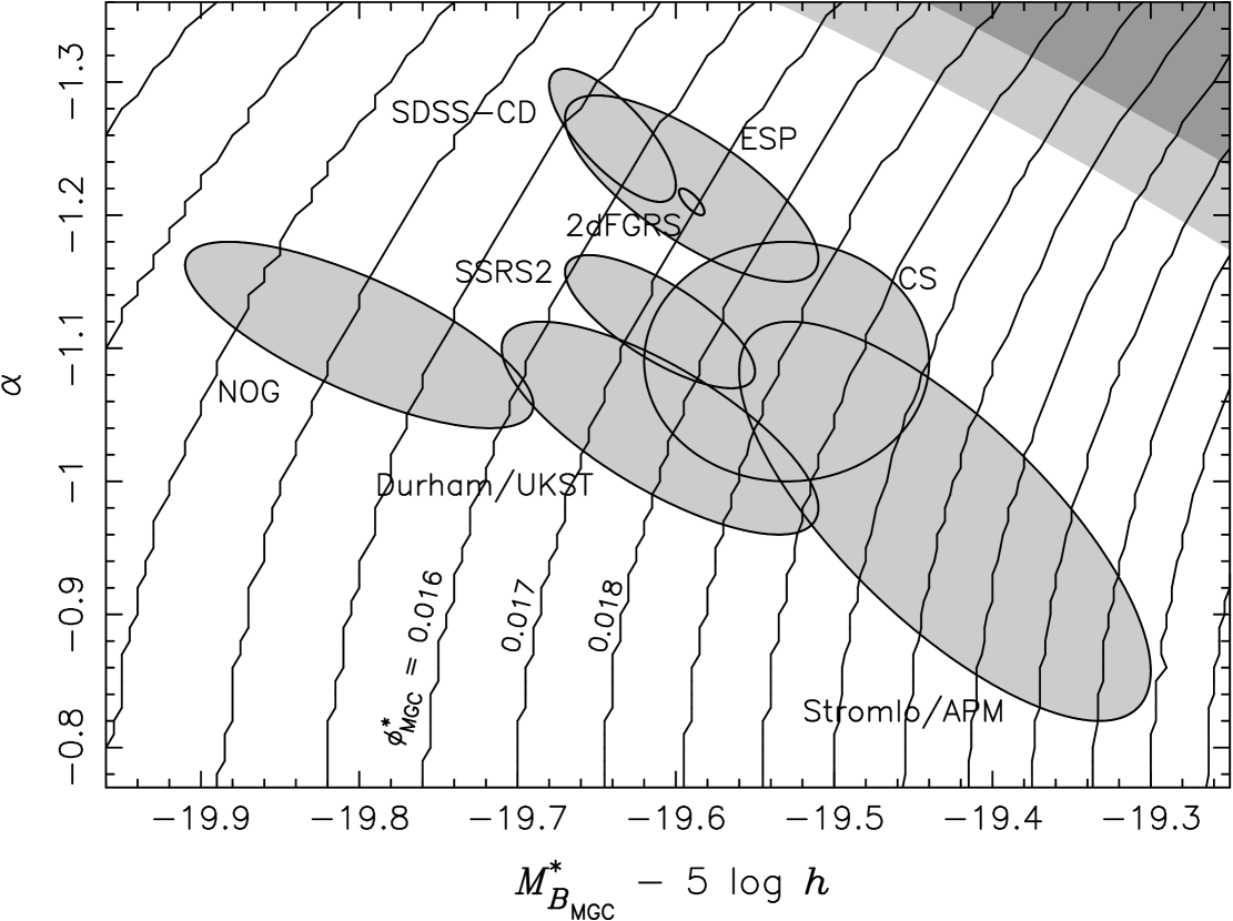
Figure 20: The contours show the best-fitting value of the LF normalization, $\phi^{*}_{\rm MGC}$, for given values of $M^{*}$ and $\alpha$. These were derived by $\chi^{2}$-minimization over the range $16\leq B_{\rm MGC}<20$ mag (cf. Fig. 19, using the full covariance matrix). The values of the contours increase from $0.011$ $h^{3}$ Mpc^-3 on the left in steps of $0.001$ to $0.027$ on the right as indicated. The error ellipses of the LFs of Table 3 in the $M^{*}$-$\alpha$ plane are also indicated (assuming a correlation coefficient of $0.75$). The corresponding best-fit $\phi^{*}_{\rm MGC}$ values are listed in Table 3. The light and dark shading in the upper right corner marks those regions in the $M^{*}$–$\alpha$ plane where the shape of the predicted counts disagrees with the data at the $90$ and $95$ per cent levels, respectively.

In particular, we derive the $\phi^{*}_{\rm MGC}$ values appropriate for the LFs listed in Table 3. The revised values and their associated probabilities are listed in columns 7 and 8 of that table. Figs. 19(c) and (d) show the resulting LFs and their predicted counts after revision. All surveys now give comparable and reasonable probabilities. Note, however, that the variation of $\phi^{*}$ among the different surveys after renormalization is no less than before. This is due to the fact that the counts constrain the combination $\phi^{*}{L^{*}}^{3/2}$ and that the variation in ${L^{*}}^{3/2}$ is comparable to that of $\phi^{*}$ before renormalization (as seen from equation 16).

In Table 3 we also list the errors on $\phi^{*}_{\rm MGC}$ induced by various sources. First, we list the statistical error derived from the $\chi^{2}$ fit. This error includes remaining uncertainties due to LSS because we have used the full covariance matrix of the counts in the fit. Secondly, we list the errors due to the uncertainties in $M^{*}$ and $\alpha$, which can be essentially read off from Fig. 20. Here we take into account that the errors on $M^{*}$ and $\alpha$ are generally highly correlated by assuming a correlation coefficient of $0.75$ (Blanton et al., 2001). Finally, we have estimated the errors resulting from uncertainties in the $k+e$-correction. This error is slightly more subtle than the previous ones. For example, increasing $k+e$ has the effect of moving the contours in Fig. 20 to the left and up but it also moves the LFs in a similar direction, thus again decreasing the original change in $\phi^{*}_{\rm MGC}$ for a given survey. Norberg et al. (2002) estimated errors on their $k+e$-correction by demanding statistical consistency between the LFs derived from their high and low-$z$ samples. Since our $k+e$ is essentially identical to theirs we also adopt their error of $\pm 18$ per cent. We estimate the resulting $\phi^{*}_{\rm MGC}$ error for a given survey by first adding $\pm 0.18(k+e)(\bar{z})$ to its $M^{*}$ value and then re-deriving $\phi^{*}_{\rm MGC}$ while using the increased (or decreased) $k+e$. As in Section 7.1 we thus approximate the effect on $M^{*}$ by evaluating $\Delta(k+e)$ at the median redshift of the survey. Comparison with Norberg et al.’s $k+e$ induced error on $M^{*}$ indicates that this procedure underestimates the effect on $M^{*}$, and hence we overestimate the error on $\phi^{*}_{\rm MGC}$. We also conservatively ignore any effect on $\alpha$, which is difficult to gauge.

7.4 The local luminosity density

Taking $M_{\odot_{b_{\rm J}}}=+5.3$ mag and using the revised LF normalizations we calculate the luminosity density, $j_{b_{\rm J}}=\phi^{*}L^{*}_{b_{\rm J}}\Gamma(\alpha+2)$. Note that we convert $M^{*}_{B_{\rm MGC}}$ to $M^{*}_{b_{\rm J}}$. The calculated values of $j_{b_{\rm J}}$ are listed in the last column of Table 3, where the errors include all the $M^{*}$, $\alpha$ and $\phi^{*}_{\rm MGC}$ uncertainties while taking into account the correlation between the errors of $M^{*}$ and $\alpha$ (with a correlation coefficient 0.75 as above) as well as the virtually perfect correlations between the second error component of $\phi^{*}_{\rm MGC}$ and the errors of $M^{*}$ and $\alpha$ and between the $k+e$ errors on $M^{*}$ and $\phi^{*}_{\rm MGC}$. We find a weighted mean $b_{\rm J}$ luminosity density of $\overline{j_{b_{\rm J}}}=(1.986\pm 0.031)\times 10^{8}\;h\;L_{\odot}$ Mpc^-3. Note that the 2dFGRS and SDSS-CD, which must be considered the most reliable LFs, give a slightly higher value of $j_{b_{\rm J}}=(2.035\pm 0.046)\times 10^{8}\;h\;L_{\odot}$ Mpc^-3.

7.5 Constraints on $M^{*}$ and $\alpha$

In the previous section we minimized $\chi^{2}$ as a function of $\phi^{*}$ only while treating $M^{*}$ and $\alpha$ as fixed parameters. $\phi^{*}$ only affects the normalization of the predicted counts but not their shape which, in principle, also contains information. However, for the LFs listed in Table 3 the fits are already statistically acceptable (cf. column 9 of Table 3) and hence we cannot expect to derive useful limits on any other parameters.

Nevertheless, in Fig. 20 we mark as grey-shaded regions those combinations of $M^{*}$ and $\alpha$ where the adjustment of $\phi^{*}$ does not result in an acceptable fit (at the $90$ and $95$ per cent confidence levels), i.e. where the shape of the predicted counts disagrees with the data. As expected these limits cannot exclude any of the measured values.

8 Conclusions

Here we have presented a detailed description of the Millennium Galaxy Catalogue (MGC), a deep ($\mu_{\rm lim}=26$ mag arcsec^-2) wide ($37.5$ deg²) survey along the equatorial strip from $9^{\rm h}58^{\rm m}$ to $14^{\rm h}47^{\rm m}$. We have demonstrated that the internal photometric accuracy of the MGC is $\pm 0.023$ mag and that the astrometric accuracy is $\pm 0.08$ arcsec in both RA and Dec. Using SExtractor we have derived a source catalogue containing over 1 million objects spanning the range $16\leq B_{\rm MGC}<24$ mag. All non-stellar detections brighter than $B_{\rm MGC}=20$ mag have been visually inspected and the objects repaired where necessary. We have taken care to exclude objects from regions where the photometry is likely to be erroneous, resulting in a robust and clean estimation of the galaxy number counts over the range $16\leq B_{\rm MGC}<24$ mag. These data finally connect the faint pencil beam CCD surveys of the past decade to the local Universe. The selection boundaries of the MGC are well defined and to $B_{\rm MGC}=20$ mag we are demonstrably robust to star–galaxy separation and low- and high-surface brightness concerns. We contest that the MGC galaxy number counts in this range are the state of the art, superseding all previous intermediate number count data.

We use the counts to test various estimates of the galaxy luminosity function and find that many of them predict counts where the normalizations are inconsistent with our observations. In Fig. 20 we present the best-fitting value of $\phi^{*}$ as a function of $M^{*}$ and $\alpha$. In Table 3 we list the appropriate $\phi^{*}$ values for a number of popular $B$-band luminosity function estimates.

From these revised values we constrain the $b_{\rm J}$-band luminosity density of the local Universe for each of these luminosity functions. We find $\overline{j_{b_{\rm J}}}=(1.986\pm 0.031)\times 10^{8}\;h\;L_{\odot}$ Mpc^-3. The 2dFGRS and SDSS-EDR consistently give a slightly higher value of $j_{b_{\rm J}}=(2.035\pm 0.046)\times 10^{8}\;h\;L_{\odot}$ Mpc^-3.

References

- Alonso et al. (1994) Alonso M. V., da Costa L. N., Latham D. W., Pellegrini P. S., Milone A. A. E., 1994, AJ, 108, 1987
- Arnouts et al. (1997) Arnouts S., de Lapparent V., Mathez G., Mazure A., Mellier Y., Bertin E., Kruszewski A., 1997, A&AS, 124, 163
- Arnouts et al. (1999) Arnouts S., D’Odorico S., Cristiani S., Zaggia S., Fontana A., Giallongo E., 1999, A&A, 341, 641
- Babul & Rees (1992) Babul A., Rees M. J., 1992, MNRAS, 255, 346
- Bahcall (1986) Bahcall J. N., 1986, ARA&A, 24, 577
- Bahcall & Soneira (1980) Bahcall J. N., Soneira R. M., 1980, ApJS, 44, 73
- Bertin & Arnouts (1996) Bertin E., Arnouts S., 1996, A&AS, 117, 393
- Bertin & Dennefeld (1997) Bertin E., Dennefeld M., 1997, A&A, 317, 43
- Blair & Gilmore (1982) Blair M., Gilmore G., 1982, PASP, 94, 742
- Blanton et al. (2001) Blanton M. et al., 2001, AJ, 121, 2358
- Blanton et al. (2003) Blanton M. et al., 2003, ApJ, submitted, astro-ph/0210215
- Broadhurst et al. (1988) Broadhurst T. J., Ellis R. S., Shanks T., 1988, MNRAS, 235, 827
- Brown et al. (2001) Brown W. R., Geller M. J., Fabricant D. G., Kurtz M. J., 2001, AJ, 122, 714
- Bruzual & Charlot (1993) Bruzual A. G., Charlot S., 1993, ApJ, 405, 538
- Cohen et al. (2003) Cohen S. C., Windhorst R. A., Odewahn S. C., Chiarenza C. A., Driver S. P., 2003, AJ, 125, 1762
- Cole et al. (2000) Cole S., Lacey C. G., Baugh C. M., Frenk C. S., 2000, MNRAS, 319, 168
- Colless et al. (2001) Colless M., Dalton G., Maddox S., Sutherland W., Norberg P., Cole S. et al., 2001, MNRAS, 328, 1039
- Connolly et al. (2002) Connolly A. J. et al., 2002, ApJ, 579, 42
- Corwin et al. (1985) Corwin H. G., de Vaucouleurs A., de Vaucouleurs G., 1985, Southern Galaxy Catalogue. University of Texas, Austin
- Cross (2002) Cross N. J. G., 2002, PhD thesis, University of St Andrews
- Cross & Driver (2002) Cross N. J. G., Driver S. P., 2002, MNRAS, 329, 579
- Cross et al. (2001) Cross N. J. G., Driver S. P., Couch W. J. et al., 2001, MNRAS, 324, 825
- Cross et al. (2003) Cross N. J. G., Driver S. P., Liske J., Lemon D. J., Cole S., Norberg P., Peacock J. P., Sutherland W. J., 2003, MNRAS, submitted
- Davis & Huchra (1982) Davis M., Huchra J., 1982, ApJ, 254, 437
- de Vaucouleurs et al. (1991) de Vaucouleurs G., de Vaucouleurs A., Corwin H. G., Buta R. J., Paturel G., Fouqué P., 1991, Third Reference Catalogue of Bright Galaxies. Springer, Berlin
- Disney (1976) Disney M. J., 1976, Nat, 263, 573
- Drinkwater et al. (1999) Drinkwater M. J., Phillips S., Gregg M. D., Parker Q. A., Smith R. M., Davies J. I., Jones J. B., Sadler E. M., 1999, ApJ, 511, L97
- Driver (1999) Driver S. P., 1999, ApJ, 526, L69
- Driver et al. (1998) Driver S. P., Fernández-Soto A., Couch W. J., Odewahn S. C., Windhorst R. A., Phillips S., Lanzetta K., Yahil A., 1998, ApJ, 496, L93
- Driver et al. (1994) Driver S. P., Phillipps S., Davies J. I., Morgan I., Disney M. J., 1994, MNRAS, 266, 155
- Driver et al. (1995) Driver S. P., Windhorst R. A., Griffiths R. E., 1995, ApJ, 453, 48
- Efron (1982) Efron B., 1982, The Jackknife, the Bootstrap and Other Resampling Plans. Society for Industrial and Applied Mathematics, Philadelphia
- Efstathiou et al. (1988) Efstathiou G., Ellis R. S., Peterson B. A., 1988, MNRAS, 232, 431
- Ellis (1997) Ellis R. S., 1997, ARA&A, 35, 389
- Ellis et al. (1996) Ellis R. S., Colless M., Broadhurst T., Heyl J., Glazebrook K., 1996, MNRAS, 280, 235
- Ferguson & Babul (1998) Ferguson H. C., Babul A., 1998, MNRAS, 296, 585
- Fukugita et al. (1996) Fukugita M., Ichikawa T., Gunn J. E., Doi M., Shimasaku K., Schneider D. P., 1996, AJ, 111, 1748
- Gardner et al. (1996) Gardner J. P., Sharples R. M., Carrasco B. E., Frenk C. S., 1996, MNRAS, 282, L1
- Gunn et al. (1998) Gunn J. E. et al., 1998, AJ, 116, 3040
- Hambly et al. (2001) Hambly N. C. et al., 2001, MNRAS, 326, 1279
- Heydon-Dumbleton et al. (1989) Heydon-Dumbleton N. H., Collins C. A., MacGillivray H. T., 1989, MNRAS, 238, 379
- Huang et al. (2001) Huang J.-S. et al., 2001, A&A, 368, 787
- Impey & Bothun (1997) Impey C., Bothun G., 1997, ARA&A, 35, 267
- Infante et al. (1986) Infante L., Pritchet C., Quintana H., 1986, AJ, 91, 217
- Irwin & Lewis (2001) Irwin M., Lewis J., 2001, New Astronomy Review, 45, 105
- Ivezić et al. (2001) Ivezić Ž. et al., 2001, AJ, 122, 2749
- Jones et al. (1991) Jones L. R., Fong R., Shanks T., Ellis R. S., Peterson B. A., 1991, MNRAS, 249, 481
- Kirshner et al. (1978) Kirshner R. P., Oemler A., Schechter P. L., 1978, AJ, 83, 1549
- Koo (1986) Koo D. C., 1986, ApJ, 311, 651
- Koo & Kron (1992) Koo D. C., Kron R. G., 1992, ARA&A, 30, 613
- Kron (1980) Kron R. G., 1980, ApJS, 43, 305
- Kümmel & Wagner (2001) Kümmel M. W., Wagner S. J., 2001, A&A, 370, 384
- Landolt (1992) Landolt A. U., 1992, AJ, 104, 340
- Lauberts (1982) Lauberts A., 1982, ESO/Uppsala survey of the ESO(B) atlas. European Southern Observatory (ESO), Garching
- Lauberts & Valentijn (1989) Lauberts A., Valentijn E. A., 1989, The surface photometry catalogue of the ESO-Uppsala galaxies. European Southern Observatory (ESO), Garching
- Lemon et al. (2003) Lemon D. J., Wyse R. F. G., Liske J., Driver S. P., Horne K., 2003, MNRAS, submitted
- Loveday et al. (1992) Loveday J., Peterson B. A., Efstathiou G., Maddox S. J., 1992, ApJ, 390, 338
- Maddox et al. (1990a) Maddox S. J., Efstathiou G., Sutherland W. J., Loveday J., 1990a, MNRAS, 243, 692
- Maddox et al. (1990b) Maddox S. J., Sutherland W. J., Efstathiou G., Loveday J., Peterson B. A., 1990b, MNRAS, 247, 1P
- Marinoni et al. (1998) Marinoni C., Monaco P., Giuricin G., Costantini B., 1998, ApJ, 505, 484
- Marinoni et al. (1999) Marinoni C., Monaco P., Giuricin G., Costantini B., 1999, ApJ, 521, 50
- Marzke et al. (1998) Marzke R. O., da Costa L. N., Pellegrini P. S., Willmer C. N. A., Geller M. J., 1998, ApJ, 503, 617
- Metcalfe et al. (1995) Metcalfe N., Fong R., Shanks T., 1995, MNRAS, 274, 769
- Metcalfe et al. (2001) Metcalfe N., Shanks T., Campos A., McCracken H. J., Fong R., 2001, MNRAS, 323, 795
- Metcalfe et al. (1991) Metcalfe N., Shanks T., Fong R., Jones L. R., 1991, MNRAS, 249, 498
- Metcalfe et al. (1995) Metcalfe N., Shanks T., Fong R., Roche N., 1995, MNRAS, 273, 257
- Nilson (1973) Nilson P., 1973, Acta Universitatis Upsaliensis. Nova Acta Regiae Societatis Scientiarum Upsaliensis - Uppsala Astronomiska Observatoriums Annaler. Astronomiska Observatorium, Uppsala
- Norberg et al. (2002) Norberg P., Cole S., Baugh C. M., Frenk C. S. et al., 2002, MNRAS, 336, 907
- Paturel et al. (1989) Paturel G., Fouqué P., Bottinelli L., Gouguenheim L., 1989, A&AS, 80, 299
- Pearce et al. (2001) Pearce F. R., Jenkins A., Frenk C. S., White S. D. M., Thomas P. A., Couchman H. M. P., Peacock J. A., Efstathiou G., 2001, MNRAS, 326, 649
- Peebles (1980) Peebles P. J. E., 1980, Large-Scale Structure of the Universe. Princeton University Press, Princeton, New Jersey
- Peterson et al. (1986) Peterson B. A., Ellis R. S., Efstathiou G., Shanks T., Bean A. J., Fong R., Zen-Long Z., 1986, MNRAS, 221, 233
- Phillipps & Driver (1995) Phillipps S., Driver S., 1995, MNRAS, 274, 832
- Pimbblet et al. (2001) Pimbblet K. A., Smail I., Edge A. C., Couch W. J., O’Hely E., Zabludoff A. I., 2001, MNRAS, 327, 588
- Prandoni et al. (1999) Prandoni I. et al., 1999, A&A, 345, 448
- Ratcliffe et al. (1998) Ratcliffe A., Shanks T., Parker Q. A., Fong R., 1998, MNRAS, 293, 197
- Schechter (1976) Schechter P., 1976, ApJ, 203, 297
- Schlegel et al. (1998) Schlegel D. J., Finkbeiner D. P., Davis M., 1998, ApJ, 500, 525
- Shanks et al. (1984) Shanks T., Stevenson P. R. F., Fong R., MacGillivray H. T., 1984, MNRAS, 206, 767
- Sprayberry et al. (1997) Sprayberry D., Impey C. D., Irwin M. J., Bothun G. D., 1997, ApJ, 482, 104
- Stoughton et al. (2002) Stoughton C. et al., 2002, ApJ, 123, 485
- Strauss et al. (2002) Strauss M. A. et al., 2002, AJ, 124, 1810
- Tyson (1988) Tyson J. A., 1988, AJ, 96, 1
- Vorontsov-Vel’Yaminov & Arkhipova (1974) Vorontsov-Vel’Yaminov B. A., Arkhipova V. P., 1962–1974, Morphological catalogue of galaxies. Vol. 1–5, State University, Moscow
- White & Frenk (1991) White S. D. M., Frenk C. S., 1991, ApJ, 379, 52
- Williams et al. (1996) Williams R. E. et al., 1996, AJ, 112, 1335
- Yasuda et al. (2001) Yasuda N. et al., 2001, AJ, 122, 1104
- York et al. (2000) York D. G. et al., 2000, AJ, 120, 1579
- Zucca et al. (1997) Zucca E. et al., 1997, A&A, 326, 477
- Zwicky et al. (1968) Zwicky F., Herzog E., Wild P., Karpowicz M., Kowal C., 1961–1968, Catalogue of Galaxies and of Clusters of Galaxies. Vol. 1–6, California Institute of Technology, Pasadena