Realistic Ionizing Fluxes for Young Stellar Populations from 0.05 to $\mn@boldsymbol{\mathbf{2}\times Z_{\odot}}$

Abstract

We present a new grid of ionizing fluxes for O and Wolf-Rayet stars for use with evolutionary synthesis codes and single star H ii region analyses. A total of 230 expanding, non-LTE, line-blanketed model atmospheres have been calculated for five metallicities (0.05, 0.2, 0.4, 1 and 2 Z_⊙) using the WM-basic code of Pauldrach et al. (2001) for O stars and the cmfgen code of Hillier & Miller (1998) for W-R stars. The stellar wind parameters are scaled with metallicity for both O and W-R stars. We compare the ionizing fluxes of the new models with the CoStar models of Schaerer & de Koter (1997) and the pure helium W-R models of Schmutz, Leitherer & Gruenwald (1992). We find significant differences, particularly above 54 eV, where the emergent flux is determined by the wind density as a function of metallicity. The new models have lower ionizing fluxes in the He i continuum with important implications for nebular line ratios.

We incorporate the new models into the evolutionary synthesis code Starburst99 (Leitherer et al. 1999) and compare the ionizing outputs for an instantaneous burst and continuous star formation with the work of Schaerer & Vacca (1998; SV98) and Leitherer et al. (1999). The changes in the output ionizing fluxes as a function of age are dramatic. We find that, in contrast to previous studies, nebular He ii $\lambda 4686$ will be at, or just below, the detection limit in low metallicity starbursts during the W-R phase. The new models have lower fluxes in the He i continuum for $Z\geq 0.4$ Z_⊙ and ages $\leq 7$ Myr because of the increased line blanketing.

We test the accuracy of the new model atmosphere grid by constructing photoionization models for simple H ii regions, and assessing the impact of the new ionizing fluxes on important nebular diagnostic line ratios. For the case of an H ii region where the ionizing flux is given by the WM-basic dwarf O star grid, we show that He i $\lambda 5786$/H$\beta$ decreases between 1 and 2 Z_⊙ in a similar manner to observations (e.g. Bresolin et al. 1999). We find that this decline is caused by the increased effect of line blanketing above solar metallicity. We therefore suggest that a lowering of the upper mass limit at high abundances is not required to explain the diminishing strength of He i $\lambda 5786$/H$\beta$, as has been suggested in the past (e.g. Shields & Tinsley 1976; Bresolin et al. 1999). For an H ii region where the ionizing flux is provided by an instantaneous burst of total mass $10^{6}$ M_⊙, we plot the softness parameter $\eta^{\prime}$ against the abundance indicator $R_{23}$ for ages of 1–5 Myr. The new models are coincident with the observational data of Bresolin et al. (1999), particularly during the W-R phase, unlike the previous models of SV98 which generally over-predict the hardness of the ionizing radiation.

The new model grid and updated Starburst99 code can be downloaded from http://www.star.ucl.ac.uk/starburst.

1 Introduction

Evolutionary synthesis codes are commonly used to derive the properties of young, unresolved stellar populations from observations at various wavelengths. In the satellite ultraviolet, the stellar wind spectral features of a population of massive stars can be synthesized to provide information on the star formation rates, the slope of the initial mass function (IMF), and ages (e.g. Robert, Leitherer & Heckman 1993; Leitherer, Robert & Heckman 1995; de Mello, Leitherer & Heckman 2000). In the optical region, the properties of integrated stellar populations are usually derived indirectly from their total radiative energy outputs using nebular diagnostic line ratios (e.g. García-Vargas, Bressan & Díaz 1995; Stasińska & Leitherer 1996; Stasińska, Schaerer & Leitherer 2001). This method uses the theoretical ionizing fluxes from a population of massive stars as a function of age as input into a photoionization code. The ability of evolutionary synthesis models to predict correctly the properties of a young stellar population from nebular emission line ratios therefore depends heavily on the accuracy of the evolutionary and atmospheric models developed for single massive stars.

Early attempts to model stellar populations using evolutionary synthesis coupled with photoionization codes relied mainly on Kurucz (1992) plane-parallel LTE model atmospheres (e.g. García-Vargas et al. 1995). Gabler et al. (1989), however, showed that the presence of a stellar wind has a significant effect on the emergent ionizing flux in the neutral and ionized helium continua of O stars. Non-LTE effects depopulate the ground state of He ii, leading to a decrease in the bound-free opacity above 54 eV, and hence a larger flux in the He ii continuum by up to 3–6 orders of magnitude. The emergent spectrum is flattened in the region of the He i continuum and has a higher flux due to the presence of the stellar wind.

Stasińska & Leitherer (1996) were the first to use expanding non-LTE atmospheres for stars with strong winds to construct photoionization models for evolving starbursts. They used the grid of pure helium, unblanketed non-LTE W-R atmospheres from Schmutz, Leitherer & Gruenwald (1992) to represent evolved stars with strong winds, and Kurucz (1992) models for hot stars close to the main sequence. Line-blanketed, expanding non-LTE models covering the main sequence evolution of O stars were first introduced by Stasińska & Schaerer (1997) who studied the effect of using the CoStar models of Schaerer & de Koter (1997) on the ionization of single star H ii regions. They found that higher ionic ratios were obtained in comparison to Kurucz models with the same stellar temperatures. Schaerer & Vacca (1998) used the CoStar and Schmutz et al. (1992) grids to construct evolutionary synthesis models for young starbursts. They predicted strong nebular He ii $\lambda 4686$ in low metallicity starbursts containing W-R stars. The same evolutionary synthesis models were used by Stasińska, Schaerer & Leitherer (2001) combined with photoionization models to analyse the emission line properties of H ii galaxies.

One major question arises: how realistic are the ionizing fluxes being used in the evolutionary synthesis studies outlined above? To address this, there have been numerous studies aimed at empirically testing the accuracy of hot star model atmospheres by analysing H ii regions containing single stars with well defined spectral types and effective temperatures. Schaerer (2000) reviews the success of non-LTE model atmospheres in reproducing nebular diagnostic line ratios. Esteban et al. (1993) examined the accuracy of the W-R grids by photoionization modelling of nebulae ionized by single W-R stars. They found that the lack of line blanketing was most important for the coolest W-R stars. In recent years, new computational techniques have allowed line-blanketed W-R atmospheres to be calculated for a few stars (e.g. Schmutz 1997; de Koter, Heap & Hubeny 1997; Hillier & Miller 1998). Crowther et al. (1999) tested these models by seeking to find a consistent model that reproduced the stellar and nebular parameters of a cool WN star. They found that line blanketing plays a significant role in modifying the W-R ionizing output although the models of de Koter et al. (1997) and Hillier & Miller (1998) predict quite different ionizing flux distributions below the He i edge.

Bresolin, Kennicutt & Garnett (1999) modelled extragalactic H ii regions using Kurucz and non-LTE models. They find that the temperatures of the ionizing stars decrease with increasing metallicity, and suggest that this can be explained by lowering the upper mass limit for star formation. In a further study, Kennicutt et al. (2000) have analysed a large sample of H ii regions containing stars of known spectral types and effective temperatures. They confirm the dependence of stellar temperature on metallicity, although they note that this relationship depends on the correctness of the input ionizing fluxes, and particularly the amount of line blanketing. Oey et al. (2000) have presented a detailed comparison of spatially resolved H ii region spectra to photoionization models to test how well the CoStar models and Schmutz et al. (1992) W-R models reproduce the observed nebular line ratios. They find that overall the agreement is within 0.2 dex but the nebular models appear to be too hot by $\sim 1000$ K, and suggest that the ionizing flux distribution may be too hard in the 41–54 eV range. On the other hand, Kewley et al. (2001) model a large sample of infrared starburst galaxies, and find that the Schmutz et al. (1992) W-R atmospheres do not produce sufficient flux between 13.6–54 eV to match their observations.

It is clear that the use of expanding non-LTE model atmospheres in the analysis of single and unresolved H ii regions is a major improvement over using static LTE models to represent hot massive stars. The empirical studies described above show that, in addition, it is essential that the atmospheres are line-blanketed, particularly for studies of young stellar populations at solar or higher metallicities. The CoStar models used in more recent studies do incorporate line blanketing but the lack of any line blanketing in the W-R atmosphere grid of Schmutz et al. (1992) is a serious deficiency. With the recent advances in computing and the development of large codes to calculate expanding, non-LTE line blanketed atmospheres, it is now feasible to compute a grid of realistic ionizing fluxes for OB and W-R stars. In this paper, we present such a grid for five metallicities from 0.05–2 Z_⊙ for use with the Starburst99 (Leitherer et al. 1999) evolutionary synthesis code and analyses of single star H ii regions. In Section 2, we present the details of the model atmosphere grid, and in Section 3, we compare the predicted ionizing fluxes with previous single star models used in synthesis codes. In Section 4, we incorporate the new grid into Starburst99, and in Section 5, we examine the changes in the ionizing fluxes as a function of age for an instantaneous burst and continuous star formation. In Section 6, we use the photoionization code cloudy (Ferland 2002) to assess the differences in the nebular diagnostic line ratios of H ii regions ionized by single O stars and synthetic clusters as a function of age. We discuss our results in Section 7 and present the conclusions in Section 8.

2 The Model Atmosphere Grid

We have sought to compute a grid of expanding, non-LTE, line-blanketed model atmospheres that cover the entire upper H-R diagram for massive stars with stellar winds. To this end, we have used two model atmosphere codes: the WM-basic code of Pauldrach et al. (2001) for O and early B stars; and the cmfgen code of Hillier and Miller (1998) for W-R stars. In total, we have calculated 230 model atmospheres using a 350 MHz Pentium II PC for WM-basic and a 1.3 GHz Pentium IV PC for cmfgen. Each O and W-R model calculation typically took 3 and 9 hours to complete respectively. We have calculated the models for five metallicities: 0.05, 0.2, 0.4, 1, and 2 Z_⊙, as defined by the evolutionary tracks of Meynet et al. (1994).

Table 1: OB Dwarf Model Atmosphere Grid
					Z⊙				0.2 Z⊙				0.4 Z⊙				0.05 Z⊙				2.0 Z⊙
Model	$T_{\rm{eff}}$	$\log g$	$R_{\star}$	SpT	log $\dot{M}$		$v_{\infty}$		log $\dot{M}$		$v_{\infty}$		log $\dot{M}$		$v_{\infty}$		log $\dot{M}$		$v_{\infty}$		log $\dot{M}$		$v_{\infty}$
Ref.	(kK)	(cm s-2)	(R⊙)		Q0	Q1		Q2	Q0	Q1		Q2	Q0	Q1		Q2	Q0	Q1		Q2	Q0	Q1		Q2
OB#1	50.0	4.00	9.8	O3V	-5.85		3150		-6.41		2550		-6.17		2790		-6.89		2130		-5.61		3440
					49.5	48.8		45.8	49.5	49.0		45.6	49.5	48.9		45.7	49.6	49.1		45.4	49.5	48.8		45.6
OB#2	45.7	4.00	10.4	O4V	-6.08		2950		-6.63		2390		-6.39		2610		-7.12		1990		-5.83		3220
					49.4	48.7		45.0	49.4	48.7		45.2	49.4	48.7		45.2	49.4	48.8		45.0	49.4	48.6		44.8
OB#3	42.6	4.00	10.5	O5V	-6.24		2870		-6.80		2330		-6.55		2550		-7.28		1940		-6.00		3140
					49.2	48.5		44.4	49.2	48.6		44.2	49.2	48.5		44.3	49.2	48.6		44.2	49.2	48.5		44.5
OB#4	40.0	4.00	10.6	O7V	-6.34		2500		-6.90		2020		-6.66		2210		-7.38		1690		-6.10		2730
					49.0	48.2		43.8	49.0	48.3		43.4	49.0	48.3		43.5	49.0	48.4		43.6	49.0	48.1		37.7
OB#5	37.2	4.00	10.5	O7.5V	-6.47		2100		-7.03		1700		-6.79		1860		-7.51		1420		-6.23		2290
					48.7	47.6		37.3	48.8	47.8		42.3	48.8	47.8		42.4	48.7	47.8		42.5	48.7	47.4		38.5
OB#6	34.6	4.00	10.5	O8V	-6.64		1950		-7.20		1580		-6.96		1730		-7.68		1320		-6.40		2130
					48.5	46.6		36.3	48.4	46.9		36.7	48.4	46.8		36.7	48.4	46.7		38.7	48.4	46.7		35.4
OB#7	32.3	4.00	10.1	O9V	-6.74		1500		-7.30		1210		-7.06		1330		-7.79		1010		-6.50		1640
					47.9	45.7		34.3	48.0	45.5		34.8	47.9	45.5		34.9	48.0	45.6		34.8	48.0	45.6		33.6
OB#8	30.2	4.00	9.5	B0V	-6.92		1200		-7.48		970		-7.24		1060		-7.96		810		-6.68		1310
					47.4	44.8		32.7	47.4	44.6		33.3	47.3	44.8		33.4	47.2	44.5		33.2	47.4	44.9		32.7
OB#9	28.1	4.00	8.6	B0.5V	-6.74		800		-7.30		640		-7.06		710		-7.79		540		-6.50		870
					47.0	44.5		31.5	46.8	44.2		32.4	46.8	44.3		32.2	46.8	43.9		32.1	46.9	44.5		31.1
OB#10	26.3	4.00	8.1	B1V	-6.89		700		-7.45		560		-7.20		620		-7.93		470		-6.65		760
					46.5	43.9		30.5	46.3	43.7		31.6	46.4	43.8		31.4	46.2	43.3		30.9	46.4	44.1		…
OB#11	25.0	4.00	7.1	B1.5V	-7.08		600		-7.63		480		-7.39		530		-8.12		400		-6.83		650
					46.1	43.4		…	45.9	43.2		30.8	46.1	43.3		30.9	45.8	42.9		…	46.1	43.7		…
Notes: Mass loss rates $\dot{M}$ and terminal velocities $v_{\infty}$ are in units of M⊙ yr-1 and km s-1 respectively. $Q_{0},Q_{1}$ and $Q_{2}$ are on a log scale and represent the photon luminosity (s-1) in the H i, He i and He ii ionizing continua.

Table 2: OB Supergiant Model Atmosphere Grid
					Z⊙				0.2 Z⊙				0.4 Z⊙				0.05 Z⊙				2.0 Z⊙
Model	$T_{\rm{eff}}$	$\log g$	$R_{\star}$	SpT	log $\dot{M}$		$v_{\infty}$		log $\dot{M}$		$v_{\infty}$		log $\dot{M}$		$v_{\infty}$		log $\dot{M}$		$v_{\infty}$		log $\dot{M}$		$v_{\infty}$
Ref.	(kK)	(cm s-2)	(R⊙)		Q0	Q1		Q2	Q0	Q1		Q2	Q0	Q1		Q2	Q0	Q1		Q2	Q0	Q1		Q2
OB#12	51.5	3.88	15.2	O3I	-4.59		3150		-5.14		2550		-4.90		2790		-5.63		2130		-4.34		3440
					50.0	49.3		39.4	50.0	49.5		46.7	50.0	49.4		46.6	50.0	49.5		46.4	50.0	49.2		39.9
OB#13	45.7	3.73	18.4	O4I	-4.72		2320		-5.28		1880		-5.04		2060		-5.76		1570		-4.48		2540
					49.9	49.0		38.2	49.9	49.2		45.6	49.9	49.2		38.9	49.9	49.3		45.9	50.0	48.9		37.2
OB#14	42.6	3.67	19.7	O5I	-4.92		2300		-5.48		1860		-5.24		2040		-5.96		1550		-4.68		2510
					49.8	48.9		38.3	49.8	49.1		45.4	49.9	49.1		45.2	49.8	49.2		45.4	49.8	48.7		37.6
OB#15	40.0	3.51	21.5	O6I	-5.01		2180		-5.57		1760		-5.33		1930		-6.05		1470		-4.77		2380
					49.8	48.8		38.0	49.8	49.0		44.5	49.8	49.0		38.1	49.8	49.1		38.2	49.7	48.6		36.9
OB#16	37.2	3.40	23.6	O7.5I	-5.07		1980		-5.62		1600		-5.38		1750		-6.11		1340		-4.82		2160
					49.6	48.5		37.2	49.7	48.9		37.6	49.7	48.8		37.7	49.7	48.9		44.4	49.6	48.3		36.0
OB#17	34.6	3.29	24.6	O8.5I	-5.19		1950		-5.75		1580		-5.51		1730		-6.23		1320		-4.95		2130
					49.5	48.3		36.3	49.5	48.5		37.3	49.5	48.5		37.3	49.5	48.6		37.4	49.4	47.9		35.0
OB#18	32.3	3.23	25.5	O9.5I	-5.36		1990		-5.92		1610		-5.67		1760		-6.40		1340		-5.12		2170
					49.3	47.5		33.9	49.3	47.8		36.7	49.3	47.8		36.2	49.3	48.0		36.8	49.2	47.3		33.7
OB#19	30.2	3.14	28.1	O9.7I	-5.37		1800		-5.93		1460		-5.68		1590		-6.41		1210		-5.13		1960
					49.1	46.4		32.8	49.0	46.6		34.6	49.0	46.4		34.0	49.1	47.1		35.5	49.0	46.4		…
OB#20	28.1	3.08	27.8	B0I	-5.89		1500		-6.45		1210		-6.20		1330		-6.93		1010		-5.65		1640
					48.4	45.6		32.1	48.3	45.5		33.0	48.4	45.5		32.7	48.4	45.4		33.6	48.4	45.7		…
OB#21	26.3	2.99	26.3	B0I	-6.08		1400		-6.64		1130		-6.40		1240		-7.12		940		-5.84		1530
					47.8	45.2		…	47.5	44.8		31.8	47.6	45.0		31.5	47.6	44.6		32.2	47.8	45.3		…
OB#22	25.0	2.95	26.9	B0.5I	-6.11		1200		-6.67		970		-6.43		1060		-7.15		810		-5.87		1310
					47.6	44.9		…	47.1	44.2		31.5	47.4	44.6		…	47.1	44.2		…	47.7	45.1		…
Notes: Mass loss rates $\dot{M}$ and terminal velocities $v_{\infty}$ are in units of M⊙ yr-1 and km s-1 respectively. $Q_{0},Q_{1}$ and $Q_{2}$ are on a log scale and represent the photon luminosity (s-1) in the H i, He i and He ii ionizing continua.

2.1 O star model atmospheres

The current status of modelling O stars is reviewed by Kudritzki & Puls (2000). To calculate realistic ionizing fluxes, the effects of line blocking and blanketing have to be included in any expanding non-LTE model atmosphere code. This makes the calculation complex and computer-intensive because in an expanding atmosphere, the frequency range that can be blocked by a single spectral line is increased, and thus thousands of spectral lines from different ions overlap. Schaerer & de Koter (1997) used a Monte-Carlo approach (Schmutz 1991) which has the advantage that the influence of millions of lines on the emergent spectrum can be calculated, but the disadvantage that line broadening is not included, and thus the line blanketing in the low velocity part of the wind is underestimated. The WM-basic code of Pauldrach et al. (2001) overcomes these drawbacks by using an opacity sampling technique and a consistent treatment of line blocking and blanketing to produce synthetic high resolution spectra. We have therefore used the WM-basic code of Pauldrach et al. (2001) because of its fuller treatment of line blanketing. We discuss the differences in the predicted ionizing fluxes of the CoStar and WM-basic codes in Section 3.1.

In Tables 1 and 2, we present the model grid we have computed for O and early B dwarfs and supergiants. We defined the fundamental parameters (effective temperature $T_{\rm{eff}}$; gravity $\log g$; and photospheric radius $R_{*}$) of the stellar atmospheres using the following approach. A revised absolute visual magnitude, $M_{\rm V}$– spectral type scale for O dwarfs and supergiants was determined for Galactic and LMC stars, following the approach and references cited by Crowther & Dessart (1998) in their study of early O stars. A fit was made to individual absolute magnitudes as illustrated in Fig. 1.

Next, we adopted the revised effective temperature vs. spectral type calibration of Crowther (1998) for supergiants and dwarfs, which was updated relative to Vacca, Garmany & Shull (1996) to take account of more recent hydrostatic results which neglect stellar winds and line blanketing. There is increasing evidence that the temperature scale for O dwarfs and especially supergiants based on hydrostatic models is too high (Martins, Schaerer & Hillier 2002; Crowther et al. 2002b). Fortunately, the effect for O dwarfs is relatively small $\sim 5$ kK, but future modifications will certainly be necessary.

Figure 1: The adopted absolute magnitude $M_{V}$ – spectral type calibrations for dwarf (solid), giant (dashed) and supergiant (dotted) O stars. The symbols indicate the mean values for each spectral type for dwarfs and supergiants. The typical error on these values is $\pm 0.5$ mag.

We defined an effective temperature grid to span the domain of O and early B stars from 25 000–51 000 K, spaced at typically 0.03 dex intervals to give 11 models covering the spectral classes from O3 to B1.5. Using the $T_{\rm eff}$-bolometric correction calibration of Vacca et al. (1996) we determined bolometric magnitudes and photospheric radii for each model. Since a discrepancy remains between masses derived from spectroscopic and evolutionary models (Herrero et al. 1992), we adopted (logarithmic) mean surface gravities from Vacca et al. in all cases.

The appropriate terminal velocity $v_{\infty}$ for each model at solar metallicity was determined using the $v_{\infty}$–spectral type calibrations of Prinja, Barlow & Howarth (1990) and Lamers, Snow & Lindholm (1995). The mass loss rate $\dot{M}$ was derived from the wind momentum-luminosity relationship given by Kudritzki & Puls (2000)

$$\log\left[\dot{M}v_{\infty}\left(R_{*}/R_{\odot}\right)^{0.5}\right]=\log D_{0}+x\log\frac{L}{L_{\odot}}$$

where $\log D_{0}$ and $x=20.69,1.51$ (O I); 19.87, 1.57 (O V); and 21.24, 1.34 (early B I). Since O star winds are driven through the absorption of photospheric photons by extreme ultraviolet (EUV) metal lines, mass loss rates and terminal velocities must depend on metallicity. Radiatively-driven wind theory (e.g. Kudritzki, Pauldrach & Puls 1987) predicts that mass loss should scale with metallicity with an exponent of 0.5–1.0. Recently Vink, de Koter & Lamers (2001) predict an exponent of 0.7 using Monte Carlo modelling. We have chosen to follow the prescription of Leitherer, Robert & Drissen (1992) in scaling both $\dot{M}$ and $v_{\infty}$ with metallicity by using power law exponents of 0.8 and 0.13 respectively i.e.

$$\dot{M}_{Z}=Z^{0.8}\,\dot{M}_{\odot};\ \ \ \ \ v_{\infty,Z}=Z^{0.13}\,v_{\infty,\odot}$$

The scaled values for $\dot{M}$ and $v_{\infty}$ are given for each metallicity in Tables 1 and 2.

Table 3: WN Model Atmosphere Grid
				Z⊙				0.2 Z⊙				0.4 Z⊙				0.05 Z⊙				2.0 Z⊙
Model	$T_{\star}$	$R_{\star}$	$Y$	log $\dot{M}$		$v_{\infty}$		log $\dot{M}$		$v_{\infty}$		log $\dot{M}$		$v_{\infty}$		log $\dot{M}$		$v_{\infty}$		log $\dot{M}$		$v_{\infty}$
Ref.	(kK)	(R⊙)		Q0	Q1		Q2	Q0	Q1		Q2	Q0	Q1		Q2	Q0	Q1		Q2	Q0	Q1		Q2
WN#1	30.0	20.3	0.76	-4.93		1100		-5.49		890		-5.25		970		-5.97		740		-4.69		1200
				48.8	45.0		29.5	48.8	46.8		34.7	48.8	46.6		34.4	48.8	46.8		35.3	48.7	44.3		28.0
WN#2	32.5	17.2	0.78	-4.91		1170		-5.47		940		-5.23		1030		-5.95		790		-4.67		1280
				49.0	47.4		34.3	49.0	47.7		37.0	49.0	47.7		36.8	49.0	47.7		36.5	48.8	44.3		28.3
WN#3	35.0	14.9	0.80	-4.89		1240		-5.45		1000		-5.21		1100		-5.93		840		-4.65		1350
				49.1	47.8		37.1	49.1	48.1		37.3	49.1	48.1		37.6	49.1	48.2		36.9	49.0	47.1		34.5
WN#4	40.0	11.4	0.85	-4.83		1370		-5.39		1110		-5.15		1210		-5.87		920		-4.59		1490
				49.2	48.1		38.1	49.2	48.4		37.7	49.2	48.3		37.7	49.2	48.5		37.7	49.2	47.7		34.3
WN#5	45.0	9.0	0.91	-4.76		1520		-5.32		1230		-5.08		1340		-5.80		1020		-4.52		1660
				49.3	48.4		38.1	49.3	48.6		38.2	49.3	48.6		38.1	49.3	48.7		36.9	49.2	47.9		35.2
WN#6	50.0	7.3	0.94	-4.73		1670		-5.29		1350		-5.05		1480		-5.77		1130		-4.49		1820
				49.3	48.6		38.2	49.3	48.8		38.6	49.3	48.8		38.6	49.3	48.8		38.5	49.3	48.3		38.5
WN#7	60.0	5.1	0.98	-4.69		1960		-5.25		1580		-5.01		1730		-5.73		1320		-4.45		2140
				49.4	48.9		38.4	49.4	49.0		39.1	49.4	49.0		39.2	49.4	49.0		38.9	49.3	48.6		38.6
WN#8	70.0	3.7	0.98	-4.69		2270		-5.25		1840		-5.01		2010		-5.73		1530		-4.45		2480
				49.4	49.0		39.6	49.4	49.1		39.8	49.4	49.1		39.8	49.3	49.0		39.8	49.4	48.8		38.6
WN#9	80.0	2.8	0.98	-4.69		2550		-5.25		2060		-5.01		2260		-5.73		1720		-4.45		2790
				49.4	49.1		40.1	49.3	49.1		40.4	49.4	49.1		40.3	49.3	49.1		47.5	49.4	48.9		38.9
WN#10	90.0	2.3	0.98	-4.69		2850		-5.25		2310		-5.01		2520		-5.73		1930		-4.45		3110
				49.3	49.1		40.6	49.3	49.1		47.9	49.3	49.1		40.4	49.3	49.1		48.0	49.3	49.0		39.5
WN#11	100.0	1.8	0.98	-4.69		3120		-5.25		2530		-5.01		2760		-5.73		2110		-4.45		3410
				49.3	49.1		41.2	49.3	49.1		48.3	49.3	49.1		48.1	49.3	49.1		48.3	49.3	49.0		40.4
WN#12	120.0	1.3	0.98	-4.69		3700		-5.25		3000		-5.01		3300		-5.73		2500		-4.45		4050
				49.3	49.1		49.2	49.2	49.1		48.5	49.3	49.1		48.5	49.2	49.1		48.6	49.3	49.1		41.1
Notes: Mass loss rates $\dot{M}$ and terminal velocities $v_{\infty}$ are in units of M⊙ yr-1 and km s-1 respectively. $Q_{0},Q_{1}$ and $Q_{2}$ are on a log scale and represent the photon luminosity (s-1) in the H i, He i and He ii ionizing continua.

Table 4: WC Model Atmosphere Grid
				Z⊙				0.2 Z⊙				0.4 Z⊙				0.05 Z⊙				2.0 Z⊙
Model	$T_{\star}$	$R_{\star}$	$Y$	log $\dot{M}$		$v_{\infty}$		log $\dot{M}$		$v_{\infty}$		log $\dot{M}$		$v_{\infty}$		log $\dot{M}$		$v_{\infty}$		log $\dot{M}$		$v_{\infty}$
Ref.	(kK)	(R⊙)		Q0	Q1		Q2	Q0	Q1		Q2	Q0	Q1		Q2	Q0	Q1		Q2	Q0	Q1		Q2
WC#1	40.0	9.3	0.56	-4.72		1250		-5.28		1010		-5.04		1100		-5.76		840		-4.48		1360
				48.9	41.8		26.1	49.0	47.3		33.0	49.0	47.6		34.0	48.9	46.9		31.4	48.7	42.1		25.9
WC#2	43.0	8.0	0.56	-4.72		1380		-5.28		1110		-5.04		1220		-5.76		930		-4.48		1510
				49.0	42.1		27.5	49.1	47.7		34.8	49.1	47.9		35.4	49.0	47.5		33.4	48.8	39.6		23.8
WC#3	46.0	7.0	0.56	-4.72		1510		-5.28		1220		-5.04		1340		-5.76		1020		-4.48		1650
				49.0	46.7		31.3	49.1	48.0		36.1	49.1	47.9		34.8	49.1	48.1		36.1	48.9	42.1		26.6
WC#4	50.0	5.9	0.56	-4.72		1650		-5.28		1330		-5.04		1460		-5.76		1110		-4.48		1800
				49.1	47.5		33.1	49.1	48.3		37.0	49.1	48.1		36.6	49.1	48.4		35.3	49.0	42.2		27.3
WC#5	55.0	4.9	0.56	-4.72		1870		-5.28		1510		-5.04		1660		-5.76		1260		-4.48		2040
				49.1	47.9		31.3	49.2	48.5		37.3	49.2	48.4		37.4	49.2	48.6		40.3	49.0	42.4		28.5
WC#6	60.0	4.1	0.56	-4.72		2100		-5.28		1700		-5.04		1860		-5.76		1420		-4.48		2290
				49.1	48.1		36.7	49.2	48.7		37.6	49.2	48.6		37.5	49.2	48.7		39.9	49.0	47.9		34.8
WC#7	70.0	3.0	0.56	-4.72		2450		-5.28		1980		-5.04		2170		-5.76		1650		-4.48		2680
				49.1	48.5		37.9	49.2	48.8		38.3	49.2	48.7		37.9	49.2	48.8		40.3	49.1	47.9		32.9
WC#8	80.0	2.3	0.56	-4.72		2800		-5.28		2270		-5.04		2480		-5.76		1890		-4.48		3060
				49.2	48.6		38.2	49.2	48.9		39.9	49.2	48.8		38.6	49.2	48.9		40.3	49.1	48.2		37.3
WC#9	90.0	1.8	0.56	-4.72		3200		-5.28		2590		-5.04		2840		-5.76		2160		-4.48		3500
				49.2	48.7		38.4	49.2	48.9		42.6	49.2	48.9		39.3	49.2	48.9		46.9	49.1	48.4		38.3
WC#10	100.0	1.5	0.56	-4.72		3600		-5.28		2920		-5.04		3190		-5.76		2430		-4.48		3930
				49.2	48.8		38.8	49.2	48.9		40.7	49.2	48.9		40.3	49.1	48.9		47.7	49.1	48.5		35.6
WC#11	120.0	1.0	0.56	-4.72		4400		-5.28		3570		-5.04		3900		-5.76		3000		-4.48		4810
				49.2	48.8		39.4	49.1	48.9		48.1	49.2	48.9		47.6	49.1	48.9		48.2	49.1	48.6		38.8
WC#12	140.0	0.8	0.56	-4.72		5200		-5.28		4220		-5.04		4620		-5.76		3520		-4.48		5690
				49.1	48.9		40.0	49.1	48.9		48.8	49.1	48.9		48.2	49.0	48.9		48.4	49.1	48.7		39.1
Notes: Mass loss rates $\dot{M}$ and terminal velocities $v_{\infty}$ are in units of M⊙ yr-1 and km s-1 respectively. $Q_{0},Q_{1}$ and $Q_{2}$ are on a log scale and represent the photon luminosity (s-1) in the H i, He i and He ii ionizing continua.

To compute the models, we used version 1.16 of the WM-basic code which includes atomic models of all the important ions of 149 ionization stages of 26 elements from H to Zn. The wind structure was solved for consistently in the hydrodynamic part of WM-basic, corresponding to a velocity law with exponent $\beta\sim 0.8$. Intervention was required in order that the required mass loss rate and terminal velocity were obtained, for the stellar input parameters, via “force multipliers” which describe the radiative line acceleration. We tuned the force multipliers for each model by iteration to achieve the wind parameters given in Tables 1 and 2 ($\dot{M}$ to within 5 per cent and $v_{\infty}$ to within $\pm 100$  km s^-1). We have not included the effect of shocks in the stellar wind since shock characteristics are ill-defined across the O spectral range. The presence of shocks will increase the ionizing flux at EUV and X-ray wavelengths (see Pauldrach et al. 2001 for details). In Tables 1 and 2, we also provide the photon luminosity in the H i ($\log Q_{0}$), He i ($\log Q_{1}$) and He ii ($\log Q_{2}$) ionizing continua for each model.

2.2 W-R star model atmospheres

The basic parameters of W-R stars have been substantially revised in recent years, due to the availability of increasingly sophisticated model atmospheres that are now able to reproduce their complex emission line spectra (see e.g. reviews of Hillier (1999); Crowther (1999)).

We have calculated a grid of expanding, non-LTE, line-blanketed WN and WC model atmospheres with the cmfgen code of Hillier & Miller (1998) using what we consider to be the most appropriate parameters for these stars. Line blanketing is accounted for in this code using the concept of super-levels, with reasonably sophisticated model atoms for the dominant ionization stages, namely H, He, C, N, O, Ne, Si, S, Fe in WN stars and He, C, O, Si, Fe in WC stars. Subsequent to the completion of this grid, computational improvements permitted many other elements and ionization stages to be included in cmfgen, but tests indicate that these tend to be second order effects.

In Tables 3 and 4, we present the parameters adopted in our WN and WC grids, parameterized by the stellar temperature $T_{*}$, the stellar radius $R_{*}$ (both defined at a Rosseland optical depth of $\sim 10$; see Section 4 for a discussion of W-R temperature definitions), and the helium mass fraction $Y$. To define these parameters, we used results from recent studies presenting line-blanketed model atmosphere analyses of W-R stars. For the WN class, our main references were Herald, Hillier & Schulte-Ladbeck (2001) and Hillier & Miller (1998), supplemented by Crowther & Smith (1997) for H/He ratios. For the WC class, we were guided by the analyses of Hillier & Miller (1999), Dessart et al. (2000) and Crowther et al. (2002a). Nugis & Lamers (2000) present a compilation of the stellar parameters for 64 Galactic W-R stars and provide a good discussion of the uncertainties.

We defined a $T_{*}$ range of 30 000–120 000 K for the WNs and assigned a decreasing hydrogen content from 24 per cent (representing a cool late WN star) to 2 per cent (representing a hot WNE star with $T_{*}>60\,000$ K), plus CNO equilibrium values in all cases. For the WC stars, we chose a $T_{*}$ range of 40 000–140 000 K, and fixed C/He=0.2 and C/O=4 by number. We assumed representative luminosities of $L=3\times 10^{5}$ L_⊙ and $2\times 10^{5}$ L_⊙ for the WN and WC models respectively.

The winds of W-R stars are believed to be inhomogeneous or clumped. Evidence for this comes from observations of line profile variability (e.g. Moffat et al. 1988) and the over-prediction of the strength of the scattering wings in theoretical line profiles (Hillier 1991). The significance of clumping is that it leads to a downward revision in W-R mass loss rates although the exact amount is unclear, since line profile analyses give $\dot{M}/\sqrt{f}$ where $f$ is the volume filling factor (e.g. Hillier & Miller 1999). In an analysis of the infrared and radio continuum fluxes for a large sample of W-R stars, Nugis, Crowther & Willis (1998) derived clumping-corrected mass loss rates a factor of 3–5 lower than the smooth wind values. This study, however, used a radio sample which is biased towards higher mass loss rates, and thus the clumping factors should be viewed as upper limits (C. Leitherer, priv. comm.). Recent line profile analyses using cmfgen find good consistency using clumping factors of $f\sim 0.1$ (e.g. Dessart et al. 2000; Crowther et al. 2002a), which correspond to mass loss rates that are a factor of $\sim 3$ times lower than homogeneous models.

To derive representative mass loss rates at solar metallicity, we used the mass loss–luminosity–chemical composition relationships given by Nugis & Lamers (2000) which are based on the clumping-corrected mass loss rates of Nugis et al. (1998). Specifically for the WN stars, we used the relationship

$$\log\dot{M}=-13.60+1.63\log\frac{L}{L_{\odot}}+2.22\log Y$$

which agrees well with results of line-blanketed analyses (Crowther 2001). For WC stars, Nugis & Lamers (2000) find that their mass loss rates do show an increase with luminosity but the scatter is large. Since we have chosen constant values of $L$ and $Y$ for all WC subtypes we used the WC linear regression relation of Nugis & Lamers (2000) to give a fixed mass loss rate of $\log\dot{M}=-4.72$ at solar metallicity. To assign terminal velocities, we determined approximate spectral types and used the $v_{\infty}$–spectral type calibrations of Prinja et al. (1990).

It is not known whether the wind parameters of W-R stars scale with metallicity because the driving mechanism of their winds has not been conclusively determined, and their atmospheres are chemically enriched in the products of the CNO-cycle (WNs) and He-burning (WCs). In the past, it has usually been assumed that there is no scaling with metallicity.

Observationally, the parameters of Galactic and LMC WN stars do not show a clear metallicity dependence (Hamann & Koesterke 2000) although the factor of $\sim$ two change in metallicity may not be sufficient to reveal significant variations within the observational and modelling uncertainties. Crowther (2000) analysed one SMC WN star and again found no differences relative to comparable stars in the LMC and Galaxy, although the spread in properties was large. More recently, Crowther et al. (2002a) have studied a sample of LMC WC4 stars and derived wind densities which were $\sim$0.2 dex lower than Galactic WC stars analysed in the same manner (Dessart et al. 2000). Crowther et al. concluded that a metallicity dependence for W-R stars naturally explains the well known difference between the Galactic and LMC WC populations, since the classification diagnostic C iii $\lambda 5696$ is extremely mass-loss dependent.

Recent theoretical work also indicates that the strength of W-R winds should be metallicity dependent. Although the precise wind driving mechanism is still unsolved, it is generally believed that radiation pressure with multiple scattering is responsible. The reduction in mass loss rates through clumping has alleviated the momentum problem but the momentum transfer efficiencies still lie in the range 2–20 (Nugis & Lamers 2000). Heavy metals are critical for initiating the outflow, even for WC stars, since the high ions of C and O do not possess enough driving lines in the correct energy range (Crowther et al. 2002a). Therefore we have adopted the same power law exponent scaling as used previously for the O star models (Sect. 2.1). The weak metallicity effect identified by Crowther et al. (2002a) is consistent with the scaling in our approach.

Figure 2: The flux distribution of model WC#10 ($T_{*}=100\,000$ K) for three different assumptions about the abundances and mass loss scaling: (a) abundances and mass loss rate scaled to solar (black, solid); (b) abundances and mass loss rate scaled to $0.05$ Z_⊙ (red, dashed); and (c) $0.05$ Z_⊙ abundances but mass loss rate scaled to solar (blue, dotted). Only model (b) with wind parameters scaled to $0.05$ Z_⊙ has a significant flux below the He⁺ edge at 228 Å because of the reduced wind density. The flux is in units of ergs cm^-2 s^-1 Å^-1 measured at the stellar surface.

Observations show that nebular He ii $\lambda 4686$ emission is spatially associated with hot W-R stars in low metallicity environments (Garnett et al. 1991; Schaerer, Contini & Pinado 1999). Schmutz et al. (1992; hereafter SLG92) discuss the fact that the energy output above 54.4 eV depends on the mass loss rate. In a W-R star with a strong wind, He⁺⁺ recombines at some point, whereas there is no recombination in a weak wind, and flux is emitted above 54.4 eV. In Fig. 2, we show the flux distribution of a WC model with $T_{*}=100\,000$ K for three different assumptions about the line blanketing and wind density. It is apparent that for a solar (i.e. unscaled) mass loss rate, no ionizing photons escape below 228 Å at $Z=0.05$ and $Z=$Z_⊙. Indeed, the emergent spectra are very similar, demonstrating that the reduced line blanketing at $Z=0.05$ Z_⊙ has a small effect. In contrast, the model which has wind parameters scaled to $Z=0.05$ Z_⊙ has a significant ionizing flux below the He⁺ edge. We thus find that the wind density controls the transparency of the wind below 228 Å at a given stellar temperature and the effect of line blanketing is negligible. The photon luminosities of the models are given in Tables 3 and 4 in the form of $\log Q_{0},\log Q_{1}$ and $\log Q_{2}$. It should be noted that no models with 2 Z_⊙ abundances have significant $Q_{2}$ fluxes.

The mass loss rates in Tables 3 and 4 are corrected for clumping since they are derived from the Nugis & Lamers (2000) relationship. For consistency, we have introduced clumping into the cmfgen model atmosphere calculations by adopting a volume filling factor $f$ of 0.1 (Hillier & Miller 1999). This has no effect on the emergent flux but does make a difference to the shape of the W-R line profiles. It is possible to recover the unclumped mass loss rates by multiplying the values in Tables 3 and 4 by $1/f^{1/2}$, i.e. $\sqrt{10}$. For these calculations, we assume a standard velocity law of $v(r)=v_{\infty}(1-R/r)^{\beta}$ with $\beta=1$, and a Doppler line width of 200 km s^-1.

Since the wind density is such a critical parameter, our use of the Nugis & Lamers (2000) mass-loss-luminosity calibration deserves special mention. As discussed above, this reproduces the average mass-loss rates for strong-lined Galactic W-R stars rather well. The weak-lined W-R stars, however, fall up to $\sim$0.5 dex below this calibration. Some pathological stars have even weaker winds and are not accounted for in our calculations. Examples are HD 104994 (WN3) which Crowther, Smith & Hillier (1995) predicted to emit strongly in the He⁺ continuum, whilst nebular He ii $\lambda$4686 is observed in the H ii region G 2.4+1.4 which is associated with Sand 4 (WO, Esteban et al. 1992). LMC W-R stars known to emit strongly below $\lambda$228 Å also exist, such as Brey 2 (WN2, Garnett & Chu 1994). Fortunately, such W-R stars are relatively few in number, so it is probable that neglecting their contribution is acceptable for the large massive star population in a starburst.

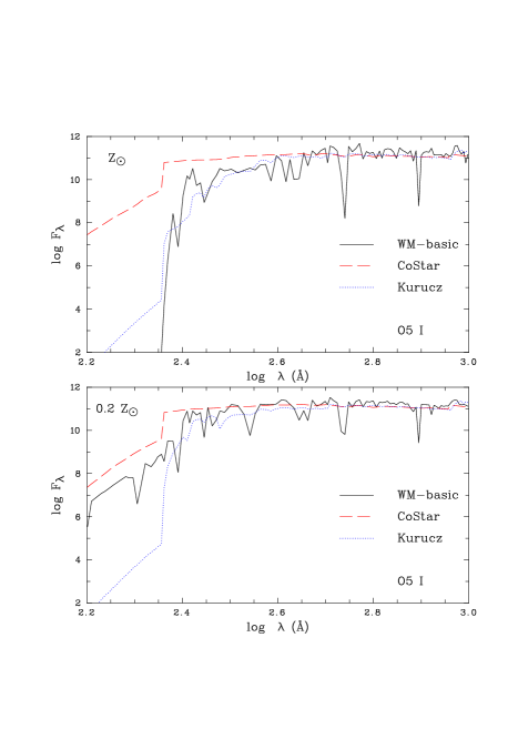
Figure 3: Comparison of the emergent fluxes for an early O supergiant from a WM-basic (black, solid), a CoStar (red, dashed), and a Kurucz model (blue, dotted) at solar metallicity and $0.2$ Z_⊙. The model details for $Z_{\odot}$ are: WM-basic OB#14 $T_{{\rm eff}}=42.6$ kK; $\log g=3.67$; $R_{*}=19.7$ R_⊙; $\log\dot{M}=-4.92$; $v_{\infty}=2300$ km s^-1; CoStar #E3 $T_{{\rm eff}}=42.6$ kK; $\log g=3.71$; $R_{*}=20.0$ R_⊙; $\log\dot{M}=-4.88$; $v_{\infty}=2538$ km s^-1; and Kurucz $T_{{\rm eff}}=42.5$ kK; $\log g=5.0$. The model parameters for $0.2$ Z_⊙ are scaled as discussed in the text.

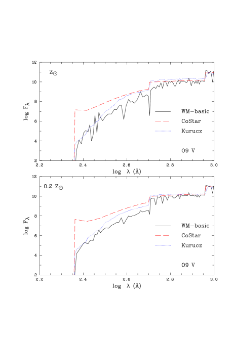
Figure 4: Comparison of the emergent fluxes for a late O dwarf from a WM-basic (black, solid), a CoStar (red, dashed), and a Kurucz model (blue, dotted) at solar metallicity and $0.2$ Z_⊙. The model details for $Z_{\odot}$ are: WM-basic OB#7 $T_{{\rm eff}}=32.3$ kK; $\log g=4.00$; $R_{*}=10.1$ R_⊙; $\log\dot{M}=-6.74$; $v_{\infty}=1500$ km s^-1; CoStar #A2 $T_{{\rm eff}}=33.3$ kK; $\log g=4.01$; $R_{*}=7.3$ R_⊙; $\log\dot{M}=-6.86$; $v_{\infty}=2544$ km s^-1; and Kurucz $T_{{\rm eff}}=32.0$ kK; $\log g=4.0$. The model parameters for $0.2$ Z_⊙ are scaled as discussed in the text.

3 Model Atmosphere Comparisons

3.1 O star models

The first expanding, line-blanketed, non-LTE grid of O star model atmospheres was introduced by Schaerer & de Koter (1997; hereafter SK97). These combined stellar structure and atmosphere or ‘CoStar’ models are used extensively in single star H ii region analyses (e.g. Oey et al. 2000) and spectral synthesis studies (e.g. Stasińska et al. 2001). The CoStar grid consists of 27 models covering the main sequence evolution of O3 to early B spectral types at metallicities of solar and 0.2 Z_⊙. The mass loss rates are taken from Meynet et al. (1994) and are scaled with metallicity using an exponent of 0.5. To compare the WM-basic with the CoStar models, we have chosen a hot (T${}_{{\rm eff}}=43$ kK; OB#14) early O supergiant model with a strong wind, and a cool (T${}_{{\rm eff}}=33$ kK; OB#7) late O dwarf model with a weak wind. In Figs. 3 and 4 we show the comparisons at solar and 0.2 Z_⊙ and also plot Kurucz (1992) LTE plane parallel models for reference. The details of the model parameters are given in the figure captions.

There are clearly significant differences in the emergent fluxes from the WM-basic and CoStar models. Considering first the O supergiant case, the WM-basic model has no flux below the He⁺ edge at Z_⊙ in contrast to the CoStar model whereas at 0.2 Z_⊙, both models have flux below 228 Å. We find again that the wind density is the critical parameter in determining the transparency below 228 Å for the WM-basic models; a model with an un-scaled (i.e. solar) mass loss rate and 0.2 Z_⊙ abundances has no flux below this wavelength (cf. Section 2.2). The reason for the difference between the CoStar and WM-basic models at $Z_{\odot}$ is less clear because both models have the same wind density. Crowther et al. (1999) explore the differences in the ionizing fluxes predicted by cmfgen and the isa-wind code of de Koter, Heap & Hubeny (1997) which is used for the CoStar atmosphere calculations. They suggest that the most likely reason for the difference is that isa-wind overestimates the far-UV flux because photon line-absorption and subsequent re-emission at longer wavelengths is not taken into account.

For the late O dwarf case, we find that the WM-basic model has a lower flux in the He⁰ continuum compared to both the CoStar and Kurucz models. It is closer to the Kurucz model, as expected for cool dwarf stars with low mass loss rates. The lower flux compared to the Kurucz model is probably due to non-LTE effects producing deeper line cores in the blocking lines (Sellmaier et al. 1996). SK97 investigated the excess flux in their dwarf models compared to plane parallel non-LTE models. They find that the temperature is too high in the region where the He⁰ continuum is formed and caution against the use of these models.

3.2 W-R models

As discussed in Section 2.2, the W-R grid is based on current best estimates of wind parameters, temperatures, luminosities and chemical compositions. These parameters differ substantially from the pure helium W-R model grid of Schmutz et al. (1992) which is implemented in the Starburst99 evolutionary synthesis code. The SLG92 grid is defined by three parameters: the ‘transformed radius’ $R_{\rm t}$ (a measure of the inverse wind density) given by

$$R_{\rm t}=R_{*}\left(\frac{10^{-4}}{dM/dt}\ \ \frac{v_{\infty}}{2500}\right)^{2/3},$$

the stellar or core effective temperature $T_{*}$, and the velocity law exponent ($\beta=1$ or 2).

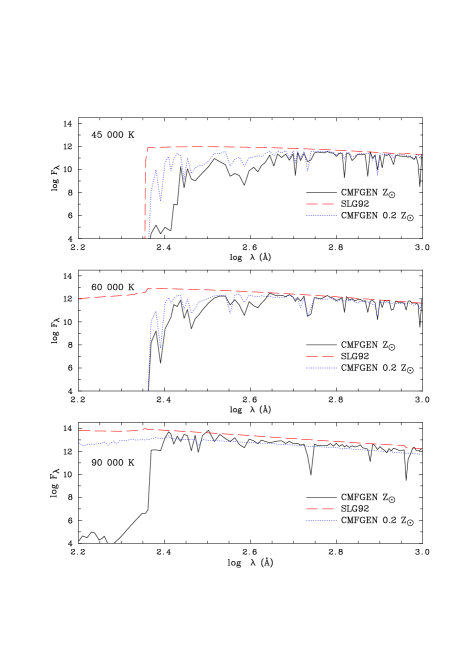
Figure 5: The emergent fluxes for cmfgen WN models with $T_{*}=45,60$ and 90 kK for $Z=$Z_⊙ (black, solid) and 0.2 Z_⊙ (blue, dotted). For comparison, the SLG92 models are also plotted (red, dashed) that would be chosen in Starburst99 for the same evolutionary point at 4 Myr in the HRD but corresponding to the hydrostatic core Meynet et al. temperatures of 56.2, 82.2 and 130.1 kK. The transformed radii $R_{\rm t}$ of these three models are 17.9, 8.4 and 1.7 R_⊙.

In Starburst99, SLG92 W-R atmospheres are connected to the evolutionary tracks by interpolating $T_{*}$ and $R_{\rm t}$ to match the hydrostatic effective temperature $T_{\rm{hyd}}$ tabulated in Meynet et al. (1994) and the $\dot{M}$ and $v_{\infty}$ values of Leitherer et al. (1992) as a function of W-R type. As discussed in the next section, the interfacing of W-R atmospheres to evolutionary tracks is difficult because of the optically thick nature of the W-R winds. We have chosen to implement the cmfgen W-R atmospheres by matching $T_{*}$ to $0.6T_{\rm{hyd}}+0.4T_{2/3}$ where $T_{2/3}$ represents the corrected temperature tabulated by Meynet et al. (1994). To make a meaningful comparison between the SLG92 and the new W-R grids, we compare models that would be selected in Starburst99 and our updated version to represent a W-R star at a given evolutionary point in the H-R diagram.

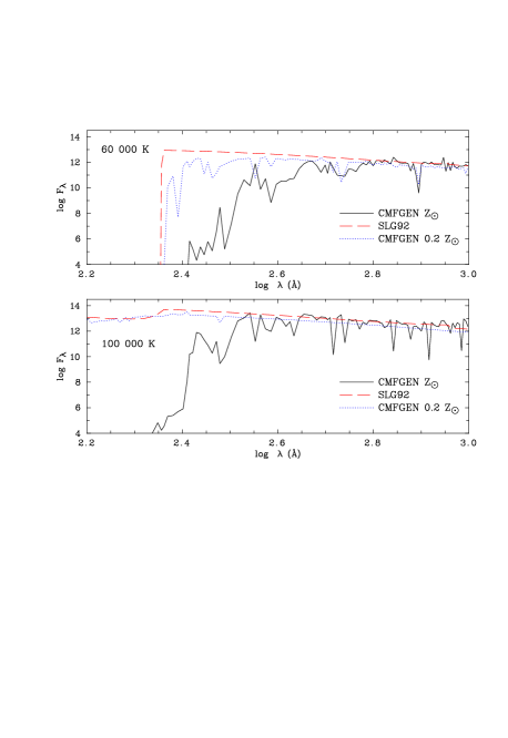
Figure 6: The emergent fluxes for cmfgen WC models with $T_{*}=60$ and 100 kK for $Z=$Z_⊙ (black, solid) and 0.2 Z_⊙ (blue, dotted). For comparison, the SLG92 models are also plotted (red, dashed) that would be chosen in Starburst99 for the same evolutionary point at 5 Myr in the HRD but corresponding to the hydrostatic Meynet et al. temperatures of 78.2 and 126.1 kK. The transformed radii $R_{\rm t}$ of these two models are 2.7 and 1.6 R_⊙.

In Fig. 5, we show three cmfgen WN models with $T_{*}=45\,000,60\,000$ and 90 000 K for metallicities of solar and 0.2 Z_⊙. For comparison, we plot the equivalent SLG92 models that would be chosen in Starburst99 at an age of 4 Myr corresponding to $T_{\rm{hyd}}=56\,200,82\,200$ and 130 100 K. Significant differences are seen because of the different wind densities, our inclusion of line blanketing, and the lower temperatures we adopt to match the W-R atmospheres to the evolutionary tracks. For the 45 000 K model, the emergent flux below 504 Å is much lower for the cmfgen model at $Z_{\odot}$ compared to SLG92 because of line blanketing, as shown by the increased flux in the $0.2$ Z_⊙ model. The 60 000 K cmfgen model has no flux below 228 Å in contrast to the higher temperature SLG92 model, and the flux below 504 Å is again reduced. The large difference in the emergent flux below 228 Å seen in Fig. 5 at 90 000 K at $Z_{\odot}$ between the cmfgen and SLG92 model is due to the wind density effect discussed in Section 2.2, since the $0.2$ Z_⊙ cmfgen model has emergent flux below 228 Å.

In Fig. 6, we plot two cmfgen WC models with temperatures of $T_{*}=60\,000$ and 100 000 K and compare them to the models that would be chosen in Starburst99 at an age of 5 Myr corresponding to $T_{\rm{hyd}}=78\,200$ and 126 100 K. The differences seen for the cooler case are similar to the 45 000 K WN model comparison in that the line blanketing at $Z_{\odot}$ produces a significant reduction in the flux in the He⁰ continuum. The differences seen at 100 000 K can be explained by the wind density determining the flux below 228 Å.

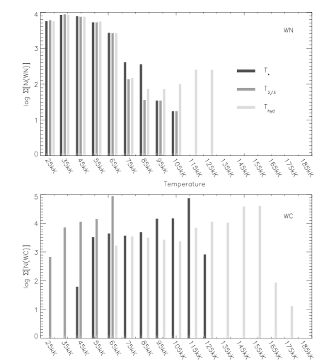
Figure 7: Histogram plots of the temperature distribution for the WN and WC phases summed over the lifetime of the W-R phase as given by Starburst99 with the Meynet et al. (1994) evolutionary tracks at solar metallicity for an instantaneous burst with $M=10^{6}$ M_⊙. For each W-R type, we show the temperature distributions corresponding to the hydrostatic temperature $T_{\rm{hyd}}$ (light grey), the corrected hydrostatic temperature $T_{2/3}$ (dark grey) of Meynet et al. (1994), and the adopted $T_{*}=0.6T_{\rm{hyd}}+0.4T_{2/3}$ (black). The temperature bin sizes are 10 kK.

4 Integration into Starburst99

Leitherer et al. (1999) present the evolutionary synthesis code Starburst99 which predicts the observable properties of galaxies undergoing active star formation, and is tailored to the analysis of massive star populations. The code is an improved version of that previously published by Leitherer & Heckman (1995). It is based on the evolutionary tracks of Meynet et al. (1994) for enhanced mass loss and the model atmosphere grid compiled by Lejeune et al. (1997), supplemented by the pure helium W-R atmospheres of Schmutz et al. (1992).

To integrate the new O star grid, we have simply replaced the Lejeune et al. (1997) LTE models by the WM-basic models for effective temperatures above 25 000 K, re-mapped to 1221 points over the wavelength range $\log\lambda=1.96$–6.20 Å, as required by the code. To ensure a smooth transition to the LTE models, we adopt the method of SV98: the WM-basic models are restricted to the $T_{{\rm eff}}$–$\log g$ domain defined by $\log g\geq 2.2$ and $\log g<5.71\times\log T_{{\rm eff}}-21.95$. The ionizing fluxes of giants were determined by averaging the supergiant and dwarf models, and renormalising to conserve the flux. Tests using real giant models show that this method is sufficiently accurate. We adopt the same method used by Leitherer et al. (1999) in choosing the best model atmosphere to represent an evolutionary point viz. selection using the nearest fit in $\log g$ and $T_{\rm{eff}}$ and then interpolation, rescaling for $T_{{\rm eff}}$ and $R$.

The new W-R grid is based on current best estimates of W-R temperatures and these are considerably lower than those of SLG92 and the evolutionary model temperatures. The problem of interfacing W-R atmospheres with evolutionary tracks is an unresolved issue which SLG92 discuss in some detail. It exists because the temperature given by evolutionary models $T_{\rm{hyd}}$ refers to the hydrostatic core. Since W-R winds are optically thick, the observed radiation emerges at larger radii, and the temperature derived from observational analyses cannot be related to $T_{\rm{hyd}}$ without inward extrapolation. To overcome this, Maeder (1990) and Meynet et al. (1994) correct the hydrostatic $T_{\rm{hyd}}$ value by assuming a velocity law to give the radius corresponding to an optical depth of 2/3 and hence a lower temperature $T_{2/3}$. This does not, however, solve the problem because the corresponding $T_{2/3}$ temperatures derived from W-R model atmospheres analyses are generally close to 30 000 K irrespective of W-R subtype. As discussed by SLG92, W-R model atmospheres are best characterized by the core temperature $T_{*}$ which refers to the radius where the optical depth is $\approx$ 10 (corresponding to a thermalization depth of unity for the continuum opacity which is dominated by electron scattering).

The problem is therefore how to assign a W-R model atmosphere characterized by $T_{*}$ to an evolutionary model defined by two temperatures: $T_{\rm{hyd}}$ and $T_{2/3}$, with the former being too hot and the latter too cool. In Starburst99, an SLG92 W-R atmosphere is assigned by interpolating $T_{*}$ and $R_{\rm t}$ to match $T_{\rm{hyd}}$ of the Meynet et al. (1994) evolutionary models. Since the $T_{\rm{hyd}}$ values of Meynet et al. are higher than the new W-R grid values, we have assigned the W-R models to the tracks by matching $T_{*}$ to $0.6T_{\rm{hyd}}+0.4T_{2/3}$. We arrived at this formalism by studying the distribution of temperatures in the W-R phase as given by Starburst99 for solar metallicity. We simply binned the number of WN and WC stars into 10 kK temperature bins and summed over the lifetime of the W-R phase. The resulting WN and WC temperature distributions are shown in Fig. 7.

For the WN stars, the temperature distribution for $T_{\rm{hyd}}$ shows one broad peak at $\sim 40\,000$ K and a second peak near 120 000 K. The distribution for the WC stars is flatter and peaks at $\sim 150\,000$ K. We first tried a simple average of the two Meynet et al. temperatures but this shifted the peak of the WN temperature distribution to a cool $\sim 30\,000$ K. We then adjusted the bias between the two temperatures by trial and error and found that $0.6T_{\rm{hyd}}+0.4T_{2/3}$ gave a single temperature distribution for the WNs peaking at 40 000 K and extending to 100 000 K. The corresponding WC temperature distribution, as shown in Fig. 7, peaks at 110 000 K. Ideally, the next step would be to compare the adopted $T_{*}$ distribution with observed W-R subtype vs. temperature distributions. Unfortunately there is insufficient data to do such a comparison. Nevertheless, our adopted $T_{*}$ values for WN and WC stars span the range occupied by Galactic and LMC W-R stars, as derived by recent analyses (e.g. Hillier & Miller 1998; Herald et al. 2001; Crowther et al. 2002a). We also note that the WN and WC $T_{*}$ peaks correspond to late WN and early WC stars. Studies of W-R galaxies (e.g. Guseva, Izotov & Thuan 2000) show that the composite W-R feature at $\sim 4680$ Å is usually dominated by these types of W-R stars.

Finally, we have adopted the same switching technique employed by Leitherer et al. (1999): W-R atmospheres are used when the surface temperature of the Meynet et al. (1994) tracks exceeds 25 000 K and the surface hydrogen content is less than 0.4. In addition, a WN or WC model is chosen depending on whether C/N$<10$ (WN) or $>10$ (WC).

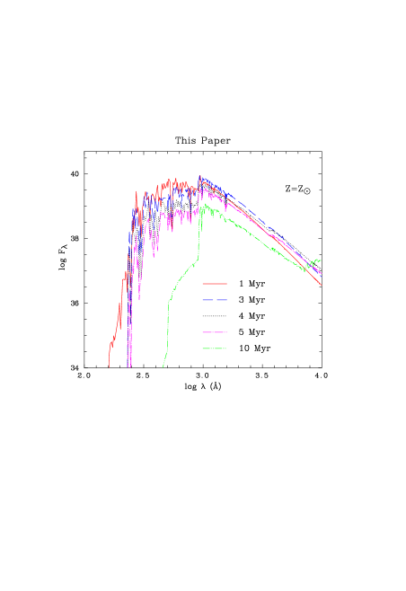
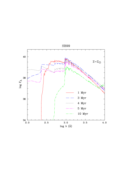
Figure 8: Spectral energy distributions of the new models (left-hand side) compared with Starburst99 (right-hand side) at time intervals of 1, 3, 4, 5 and 10 Myr for an instantaneous burst at $Z_{\odot}$.

5 Evolutionary Synthesis Comparisons

In Section 3, we compared the new O and W-R model atmospheres with the grids of Schaerer & de Koter (1997) and Schmutz et al. (1992). We find that there are significant differences below 228 Å at $Z_{\odot}$ (and higher) for the hot O supergiant and W-R models. We can thus expect large differences in the output ionizing fluxes of young massive star-forming regions, especially during the W-R phase. We compare the emergent flux distributions obtained with the new models integrated into Starburst99 to:

1. the standard version of Starburst99 (which we will refer to as SB99) which uses the W-R atmospheres of Schmutz et al. (1992) for stars with strong mass loss and the LTE models from the compilation of Lejeune et al. (1997) for all other stars.

2. a modified version of (i) with the CoStar models of Schaerer & de Koter (1997) replacing the LTE models for the main sequence evolution of massive stars. We have implemented these models as described in Schaerer & Vacca (1998) and use the solar metallicity grid for solar and above, and the $0.2$ Z_⊙ grid for $Z\leq 0.4$ Z_⊙. We refer to these models as SV98 and have checked that the output is the same as the actual SV98 models for the hot O star phase. There are small differences in the W-R phase resulting from the different methods of interpolation used in the SB99 and SV98 codes.

We consider two types of star formation: an instantaneous burst and continuous star formation. We adopt a standard initial mass function (IMF) with a single Salpeter power law slope of 2.35 and lower and upper mass cut-offs of 1 and 100 M_⊙. We use the enhanced mass loss tracks of Meynet et al. (1994) and calculate models for five metallicities: 0.05, 0.2, 0.4, 1 and 2 $Z_{\odot}$. We do not include the contribution of the nebular continuum.

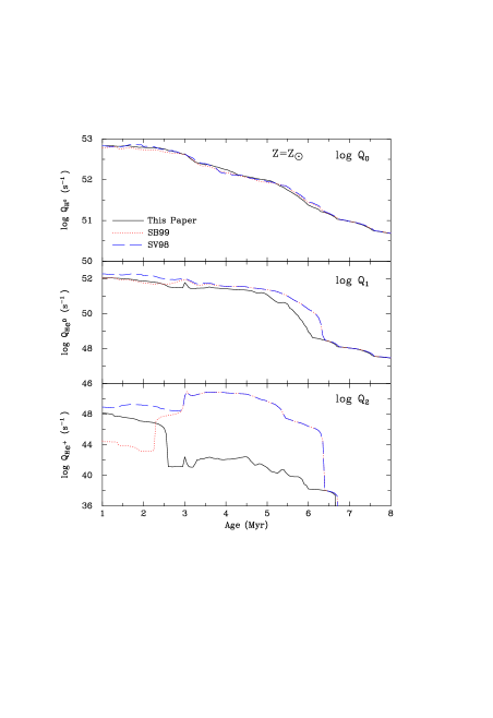
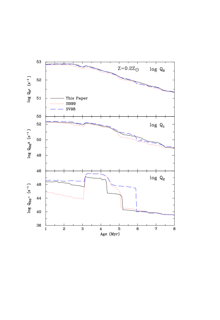
Figure 9: The evolution of the photon luminosity for ages of 1–8 Myr in the ionizing continua of hydrogen ($\log Q_{0}$), He i ($\log Q_{1}$) and He ii ($\log Q_{2}$) at 0.2 and $Z_{\odot}$ for an instantaneous burst at time steps of 0.1 Myr. The new models (black, solid) are compared to the ionizing fluxes of: Starburst99 (SB99, red, dotted) using the stellar library of Lejeune et al. (1997) and the Schmutz et al. (1992) W-R models; the Schaerer & Vacca (1998) models (SV98, blue, dashed) using CoStar and Schmutz et al. (1992) W-R atmospheres.

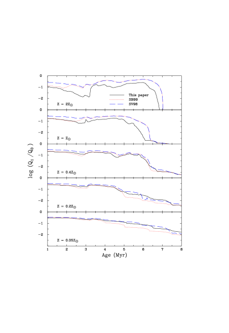
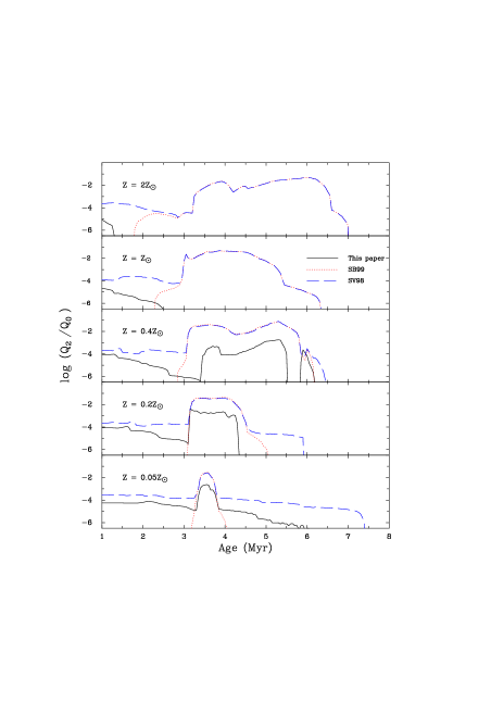
Figure 10: The evolution of the hardness of the ionizing spectra shown by the ratios of $\log(Q_{1}/Q_{0})$ (lefthand side) and $\log(Q_{2}/Q_{0})$ (righthand side) at all five metallicities for an instantaneous burst and ages of 1–8 Myr. The details of the models are given in Fig. 9.

5.1 Instantaneous burst

We adopt a standard instantaneous burst model with a total mass of $10^{6}$ M_⊙. In Fig. 8, we show the spectral energy distributions obtained with the new model atmospheres compared with SB99 at time intervals of 1, 3, 4, 5 and 10 Myr for $Z_{\odot}$. The most dramatic differences occur below the He⁺ edge at 228 Å during the W-R phase at 3–5 Myr. The new line-blanketed models have negligible flux below 228 Å at $Z_{\odot}$ in contrast to the very hard ionizing fluxes of the SLG92 atmospheres. The detailed differences between the new models and previous work, and their dependence on metallicity are best seen by considering the ionizing fluxes and their ratios. In Fig. 9, we show the evolution of the photon luminosity from 1–8 Myr in the ionizing continua of H i ($\log Q_{0}$), He i ($\log Q_{1}$) and He ii ($\log Q_{2}$) for 0.2 and $Z_{\odot}$. The evolution of the hardness of the ionizing spectra $\log(Q_{1}/Q_{0})$ and $\log(Q_{2}/Q_{0})$ for all five metallicities is shown in Fig. 10. The variation with metallicity is primarily due to the changing W-R/O ratio. The relative number of W-R stars formed and the duration of the W-R phase increases with metallicity because the lower mass limit for their formation decreases (Meynet 1995). The W-R/O ratio changes from 0.025 to 0.36 between $Z=0.05$–2 Z_⊙ at 3 Myr (SV98).

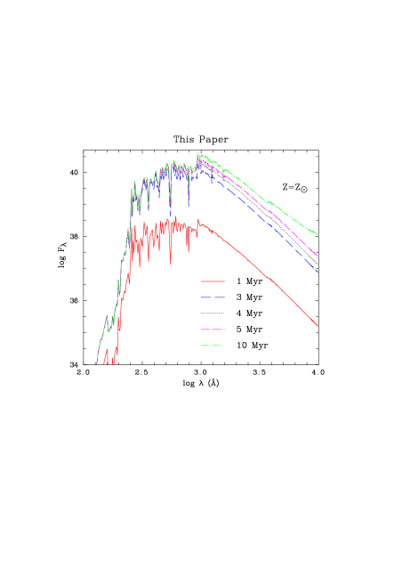
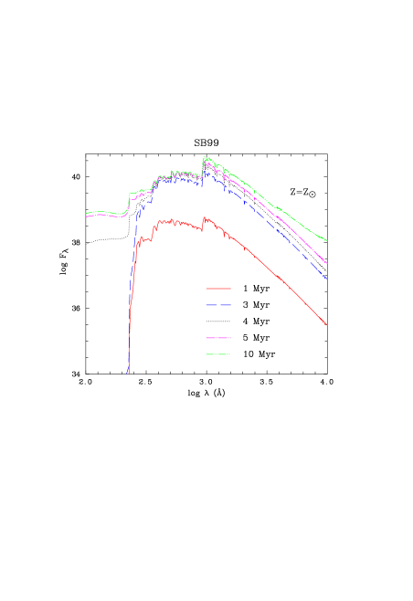
Figure 11: Spectral energy distributions of the new models (left-hand side) compared with Starburst99 (right-hand side) at time intervals of 1, 3, 4, 5 and 10 Myr for continuous star formation at $Z_{\odot}$.

The ionizing flux in the Lyman continuum $Q_{0}$ is determined mainly by hot main sequence stars. Fig. 9 shows that $Q_{0}$ is very similar to SV98 although the SB99 values are slightly lower because the Kurucz LTE models for hot O stars have smaller radii than the non-LTE O star models. The new models have lower ionizing fluxes below 504 Å at ages of less than $\sim$ 7 Myr for metallicities $\geq 0.4$ Z_⊙. This is because W-R stars contribute an important fraction of the He i ionizing flux and our new W-R models are line-blanketed compared to the SLG92 grid used for the SB99 and SV98 models. The new O star models also have a lower ionizing flux in the He i continuum (Sect. 3.1). The dependence of $\log(Q_{1}/Q_{0})$ on metallicity is demonstrated in Fig. 10. At 5 Myr, the ratio $Q_{1}/Q_{0}$ is softer by a factor of 2 at 2 Z_⊙ compared to SB99 and SV98 because of the effect of the W-R line-blanketed atmospheres, whereas at $Z=0.05$ Z_⊙, the models agree with SV98 because at this low metallicity, the main contributors to $Q_{1}$ are O supergiants because of the low W-R/O ratio. In general, at sub-solar metallicities for $Q_{1}/Q_{0}$, the new models agree more closely with SV98 than SB99.

The most pronounced revisions are seen in $Q_{2}$ during the W-R phase at 3–6 Myr in Fig. 9 for Z_⊙. The number of He ii ionizing photons emitted is now negligible compared to SV98 and SB99 because of the W-R wind density effect (Sect. 2.2) and the conspicuous bump in the SV98 and SB99 models disappears. At metallicities below solar, $Q_{2}/Q_{0}$ (Fig. 10) is softer in the W-R phase compared to SV98 and SB99 by, for example, a factor of $\sim 25$ at 0.4 Z_⊙. The W-R subtypes can be identified since we have used different models for the WN and WC phases. At 0.4 Z_⊙, the first W-R stars to form at 3.5 Myr are the late WN stars, the descendants of the most massive O stars. These stars then evolve to WC stars, and finally, near the end of the W-R phase, the O stars near the minimum mass limit for W-R formation, become WN stars. At $Z=0.05$ Z_⊙, the W-R phase is short-lived because only the most massive O stars evolve into W-R stars. At all metallicities, the new O star models are softer compared to SV98 because the far-UV flux in the CoStar atmospheres is probably overestimated (see discussion in Sect. 3.1).

Overall, at metallicities of solar and higher, we find that the He ii ionizing flux is negligible because of the high wind densities and significant line-blanketing. He ii ionizing photons are produced during the W-R phase at metallicities below solar but $Q_{2}/Q_{0}$ is much softer by a factor of $\sim 20$ compared to the SLG92 W-R models. In Section 7, we discuss the presence of nebular He ii $\lambda 4686$ as an indicator of a significant W-R population and its strength as a function of metallicity.

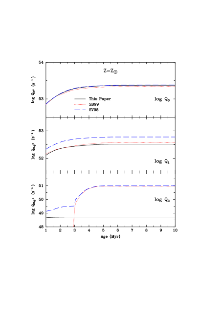
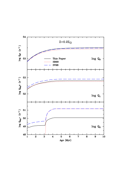
Figure 12: The evolution of the photon luminosity for ages of 1–10 Myr in the ionizing continua of hydrogen ($\log Q_{0}$), He i ($\log Q_{1}$) and He ii ($\log Q_{2}$) at 0.2 and $Z_{\odot}$ for continuous star formation at time steps of 0.1 Myr. The details of the models are given in Fig. 9.

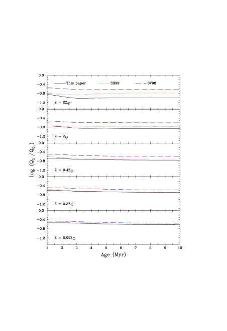
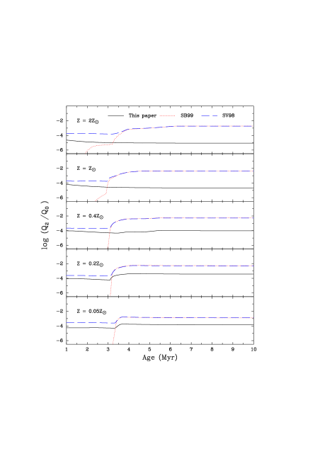
Figure 13: The evolution of the hardness of the ionizing spectra shown by the ratios of $\log(Q_{1}/Q_{0})$ (lefthand side) and $\log(Q_{2}/Q_{0})$ (righthand side) at all five metallicities for continuous star formation and ages of 1–10 Myr. The details of the models are given in Fig. 9.

5.2 Continuous star formation

For continuous star formation, we assume a star formation rate of 1 M_⊙ yr^-1 and the same IMF parameters adopted for the instantaneous case. In Fig. 11, we show the spectral energy distributions for continuous star formation. In Figs. 12 and 13, the $\log Q$ values and their log ratios are shown. After $\sim$ 5  Myr, a balance is achieved between massive star birth and death and the ionizing fluxes become time independent.

The differences shown between the various models in Fig. 12 emphasize the differences between non-LTE and LTE models and blanketed vs. un-blanketed non-LTE models. Again, the predicted values of $Q_{1}$ are lower than SV98 because of our use of line-blanketed W-R models and the lower ionizing fluxes of the WM-basic models. The difference in $Q_{2}$ for ages $<4\,$Myr between the SB99 and SV98 models is simply due to LTE vs. non-LTE models being used for O stars. The increase in $Q_{2}$ when the first W-R stars are formed is much less marked compared to SB99 and SV98 because of our use of line-blanketed W-R models. The low value of $\log Q_{2}/Q_{0}\approx-4$ implies that nebular He ii will not be detectable at any metallicity from an integrated stellar population undergoing continuous star formation (Sect. 7).

6 Impact on Nebular Diagnostics

We now assess the impact of the new grid of model atmospheres on the ionization structure of H ii regions by considering single O star and synthetic cluster models as a function of age. To perform these tests, we have used the photoionization code cloudy (version 96, Ferland 2002).

6.1 Single star H ii regions

Many studies of the excitation of H ii regions have suggested that the ionizing continuum becomes softer with increasing metal abundance (e.g. Shields 1974; Stasińska 1980; Vílchez & Pagel 1988). Shields & Tinsley (1976) first suggested that this relationship could be explained by a metallicity-dependent upper mass limit for star formation. Recently, Bresolin et al. (1999) and Kennicutt et al. (2000) have confirmed the decrease in effective temperature with increasing metal abundance. They discuss the possibility of a lower upper mass limit operating at abundances above solar, although they caution that insufficient line blanketing in the model atmospheres at high abundances may be the root cause. We are now able to test this since our new O star grid contains fully line-blanketed models up to 2 Z_⊙.

The nebular line ratio He i $\lambda 5786$/H$\beta$ is a sensitive diagnostic of the stellar temperature over the narrow range where helium is partially ionized, corresponding to $\approx$ 35 000–40 000 K, but is insensitive to changes in the ionization parameter $U$ (Bresolin et al. 1999). Using the appropriate O dwarf models listed in Table 1, we have calculated simple dust-free, plane-parallel, ionization-bounded photoionization models with $\log U=-3.0$ and a constant gas density $n=50$ cm^-3 with a filling factor of unity. We adopt the abundances and depletion factors given by Dopita et al. (2000) for solar metallicity and scale these for other metallicities. For the helium abundance as a function of metallicity, we use the formula given by Dopita et al. (2000). To compare our results with the CoStar models, we have used the model grid available within cloudy corresponding to main sequence stars for metallicities of 0.2 Z_⊙ and $Z_{\odot}$, and interpolated to match the temperatures of the WM-basic models. For Kurucz LTE models, we have used models that are the closest match to the WM-basic models in effective temperature and $\log g$.

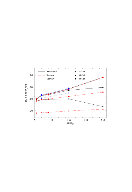
Figure 14: The predicted nebular He i $\lambda 5786$/H$\beta$ ratio plotted against metallicity for effective temperatures between 37–45kK for WM-basic, CoStar and Kurucz O V model atmospheres.

In Fig. 14, we plot He i $\lambda 5786$/H$\beta$ against metallicity for three temperatures: 37 000, 40 000 and 45 000 K. At the lower two temperatures, He is partially ionized and thus sensitive to changing effective temperature. For the WM-basic models, He becomes completely ionized at temperatures $\geq 43\,000$ K. Considering the lower two temperatures only, the Kurucz data points increase gradually with abundance. Since the observed He i $\lambda 5786$/H$\beta$ ratio shows a decrease with increasing abundance (e.g. Bresolin et al. 1999), this has led to the suggestion that effective temperature decreases with increasing $Z$. We see, however, that the WM-basic model predictions are not flat but show a decrease between 1 and 2 Z_⊙. This is because our new line-blanketed models have a softer ionizing flux in the He i continuum at high $Z$ (Fig. 10) because of the deeper line-core depths in non-LTE. The strength of He i $\lambda 5876$ for a given effective temperature therefore decreases with increasing metal abundance in a similar fashion to the observations.

The second significant difference between the WM-basic and the Kurucz and CoStar models is the large offset in the effective temperature for a given He i line strength at a single metallicity. For example at $Z_{\odot}$, at a temperature of 37 000 K, He i $\lambda 5786$/H$\beta=$ 0.10 (WM-basic); 0.12 (CoStar); and 0.05 (Kurucz). The absolute effective temperatures therefore depend heavily on the model atmospheres employed.

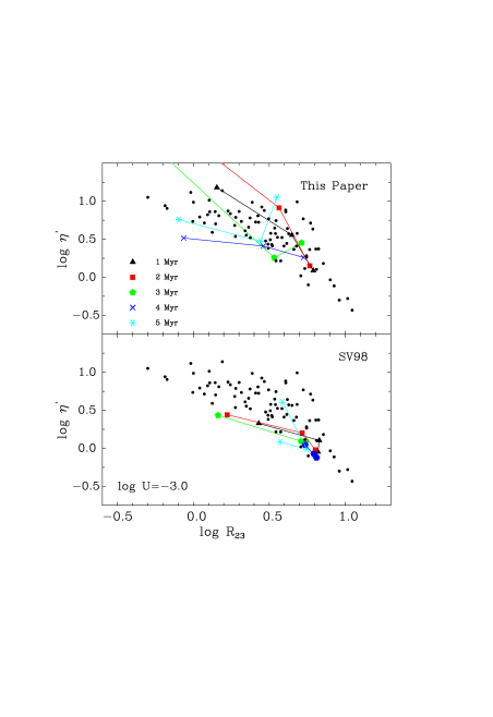
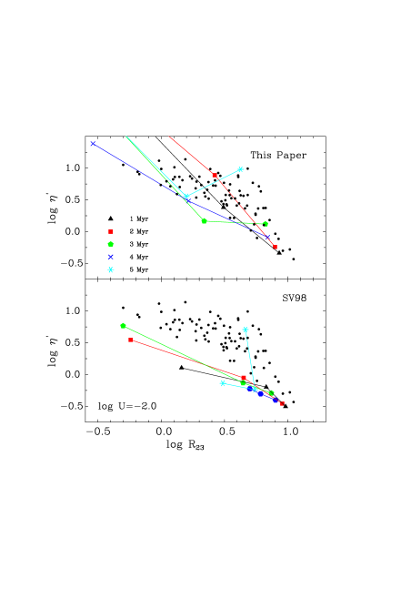
Figure 15: The predicted strength of the softness parameter $\eta^{\prime}$ plotted against the abundance indicator $R_{23}$ for 2, 1 and 0.2 $Z_{\odot}$ for cluster models with $\log U=-3$ and $-2$ using (a) the models in this paper and (b) the CoStar and SLG92 models of SV98. The observed data points for the extragalactic H ii region sample of Bresolin et al. (1999) are shown for comparison.

6.2 Cluster models

Bresolin et al. (1999) compared observational diagnostic diagrams for extragalactic H ii regions with the predictions of the cluster models of Leitherer & Heckman (1995). They found that the observed line ratios could only be reproduced for ages of 1 and 2 Myr, and concluded that either the W-R ionizing continua are too hard, or the H ii regions are disrupted at a young age. More recently, Bresolin & Kennicutt (2002) studied a sample of metal-rich extragalactic H ii regions. Some of these objects have W-R features in their spectra but the nebular line ratios are not affected i.e. they find no observational evidence that H ii regions ionized by clusters containing W-R stars show any signs of harder ionizing fluxes.

In Fig. 15, we plot the “radiation softness” parameter $\eta^{\prime}$ defined by Vílchez & Pagel (1988) as

$$\eta^{\prime}=\frac{[{\rm O\,II}]\,\lambda\lambda 3726,3729/{\rm[O\,III]}\,\lambda\lambda 4959,5007}{{\rm[S\,II]}\,\lambda\lambda 6717,6731/{\rm[S\,III]}\,\lambda\lambda 9069,9532}$$

against the abundance parameter $R_{23}=$([O II] $\lambda 3727+$[O III] $\lambda\lambda 4959,5007)/$H$\beta$. The $\eta^{\prime}$ parameter is a sensitive measure of the softness of the radiation field and provides an excellent test of the correctness of our new models. We show the predicted values of $\eta^{\prime}$ for metallicities of 2, 1 and 0.2 Z_⊙ and ages of 1–5 Myr (i.e. up to the end of the W-R phase) for an instantaneous burst model of mass $10^{6}$ M_⊙. We have used the same photoionization model parameters as in Sect. 6.1 and since $\eta^{\prime}$ is sensitive to the ionization parameter, we show two cases with $\log U=-3$ and $-2$. We compare the predictions of the new grid with the CoStar and SLG92 W-R models of SV98 and the observational data of Bresolin et al. (1999). It can be seen that the SV98 models are too hard, particularly for the $\log U=-2.0$ case, whereas the new models are coincident with the data points. We conclude that, for the parameter range explored, the ionizing fluxes of the new models are in much better agreement with the observed emission line ratios of H ii regions than previous model grids.

7 Discussion

The success of the technique of evolutionary synthesis for deriving the properties of young stellar populations depends on the accuracy of the model atmospheres and evolutionary tracks for massive stars. In this paper, we have sought to provide a grid of realistic ionizing fluxes for O and W-R stars using the latest line-blanketed, non-LTE atmosphere codes. We have carefully chosen the input stellar parameters to reflect current values available in the literature. While these appear to be well established for the O spectral class, there have been major revisions for the W-R stars. We have incorporated these changes by using lower clumping-corrected mass loss rates and lower temperatures compared to the previous W-R grid of SLG92. We have also introduced metallicity-dependent mass loss rates because recent observational and theoretical work indicate that the strength of W-R winds should scale with heavy metal abundance (Crowther et al. 2002a).

The lower, metallicity-dependent, W-R mass loss rates have implications for the amount of mass and energy returned to the interstellar medium from young starbursts. We will address this topic in a future paper. Briefly, in comparison to Leitherer et al. (1992), we find that W-R stars no longer dominate the energy input, particularly at low metallicity. Our revised O star mass loss rates, however, are larger than those given by the analytical formula of Leitherer et al. (1992), and this leads to an overall increase in the rates of mass and energy input.

As discussed in Section 3 and SLG92, the emergent flux below 228 Å depends on the wind density and hence the scaling law used to scale the wind parameters with metallicity. The precise scaling even for O stars has not been determined empirically and relies on the predictions of radiatively-driven wind theory. It is of course unknown for W-R stars and we simply chose to use the O star scaling law. The predicted number of He⁺ ionizing photons at metallicities below solar should therefore be considered as rather uncertain.

We now discuss the presence of nebular He ii $\lambda 4686$ emission. Guseva et al. (2000) compile a list of 30 H ii galaxies with nebular He ii detections. Schaerer (1996) used CoStar and the SLG92 models to synthesize the strength of nebular He ii $\lambda 4686$ emission in the early stages of a starburst. Schaerer predicts that strong nebular He ii emission will be present during the W-R phase with $I$(He ii)/$I$(H$\beta$)$=0.01$–0.025 for $0.2$ Z${}_{\odot}\leq Z\leq Z_{\odot}$. Guseva et al. (2000) find that the predicted He ii emission line strengths (as given by SV98) agree reasonably well with the observations except that the SV98 models predict the highest $I$(He ii)/$I$(H$\beta$) ratios to occur at 1 and 2 $Z_{\odot}$, while no nebular He ii is detected in objects with $Z>0.2$ Z_⊙. They also find that W-R stars cannot be the sole source of nebular He ii emission since only 60 per cent of their sample have W-R stars present, and they suggest additional mechanisms such as radiative shocks are needed to explain all the observations.

Assuming case B recombination and an ionization-bounded nebula, the strength of He ii $\lambda 4686$ relative to H$\beta$ is given by $I$(He ii)/$I$(H$\beta$)$=2.14\,Q_{2}/Q_{0}$ (SV98). If we further assume that the minimum detectable $I$(He ii)/$I$(H$\beta$)$=0.01$, then $\log Q_{2}/Q_{0}\geq-2.33$ for He ii $\lambda 4686$ to be observable. From Fig. 10, the highest value of $\log Q_{2}/Q_{0}=-2.4$, corresponding to $I$(He ii)/$I$(H$\beta$)$=0.08$, occurs at the beginning of the W-R phase at 0.2 Z_⊙. Thus any nebular He ii will be marginally observable. With the current grid of line-blanketed W-R models, it seems unlikely that the observed nebular He ii associated with W-R galaxies is in general due to W-R star photoionization.

We must emphasize that the W-R grid is based on the observational parameters of “normal or average” W-R stars and thus excludes the rare, hot early WN and WO stars with weak winds and significant fluxes above 54 eV. Since we do not understand the reasons for their extreme parameters, it is impossible to predict their impact on the ionizing output of young starbursts. Given their rarity in the Galaxy and LMC, we expect their influence to be negligible. But, if for example, they are formed via the binary channel in significant numbers at low $Z$, they may become an important source of He⁺ ionizing photons. We have also neglected shocks in the stellar winds; they will increase the ionizing flux in the EUV. It is not known how the strength of these shocks (caused by instabilities in the line-driving force) will scale with metallicity.

The problem of assigning W-R atmospheres to evolutionary models is a long-standing one and has been extensively discussed by SLG92 and in Section 3.2. To connect our new W-R models to the evolutionary tracks, we matched $T_{*}$ to $0.6T_{\rm{hyd}}+0.4T_{2/3}$ rather than matching $T_{*}$ directly to $T_{\rm{hyd}}$, as in Leitherer et al. (1999) because of the lower temperatures of the new W-R grid. The differences we find for starbursts in the W-R phase compared to the results of SV98 and Leitherer et al. (1999) is therefore potentially a combination of the effects of line blanketing and using lower temperature W-R models. The overall effect of the method we have used to connect the new W-R grid with the evolutionary tracks can be gauged from Figs. 9 and 10. The relative heights of the WN and WC bumps at $\sim$ 3.5 and 5 Myr are very similar for all three comparisons. This suggests that the main differences we find in the W-R phase are primarily due to the inclusion of line-blanketing and that the lower temperatures are a secondary effect. The formalism that we used to interface the W-R grid to the evolutionary tracks should, however, be considered as rather uncertain. For this reason, it is treated as a free parameter in the up-dated Starburst99 code.

Finally, we mention that the predictions we have made for the W-R phase as a function of metallicity depend on the evolutionary tracks of Meynet et al. (1994) for single stars with enhanced mass loss rates. Leitherer (1999) has compared various W-R synthesis models and discusses the differences in single and binary models. He finds that the W-R/O and WC/WN ratios are highest when the enhanced mass loss tracks are used, and that the W-R phase extends to between 6 and 10 Myr when binary formation is included (see also SV98). Recent evolutionary models including rotation (Maeder & Meynet 2000) have removed the necessity of artificially increasing the mass loss rate to obtain better agreement with observations of W-R stars. The lifetime of the W-R phase is increased, the WC/WN ratio is reduced, and more W-R stars are produced at low $Z$ (Maeder & Meynet 2001). The next stage in improving evolutionary synthesis models should be the inclusion of evolutionary models with rotation.

8 Conclusions

We have presented a large grid of non-LTE, line-blanketed models for O and W-R stars covering metallicities of 0.05, 0.2, 0.4, 1 and 2 Z_⊙. The grid is designed to be used with the evolutionary synthesis code Starburst99 (Leitherer et al. 1999) and in the analysis of H ii regions ionized by single stars. We have computed 110 models for O and early B stars using the WM-basic code of Pauldrach et al. (2001). The OB stellar parameters are defined at solar metallicity and are based on the most recent compilations of observational data. The mass loss rates and terminal velocities have been scaled according to metallicity by adopting power law exponents of 0.8 and 0.13 (Leitherer et al. 1992).

For the W-R grid, we used the model atmosphere code cmfgen of Hillier & Miller (1998) and computed 60 WN and 60 WC models. The new grid is based on what we consider to be the most realistic parameters derived from recent observations and individual model atmosphere analyses. In particular, the upper temperature limit of the grid is 140 000 K since the vast majority of W-R stars that have been analysed fall below this value. For the W-R mass loss rates at solar metallicity, we used the relationships derived by Nugis & Lamers (2000) which are corrected for inhomogeneities in the W-R winds. For the first time, we have introduced a W-R wind/metallicity dependence and adopted the same power law exponents used for the O star models. We argue in Sect. 2.2 that recent theoretical and observational work indicate that the strengths of W-R winds must depend on metallicity. We stress that the new W-R grid excludes the few known examples of individual hot W-R stars with weak winds that have significant ionizing fluxes above 54 eV. Since they are so rare (in the Galaxy and LMC, at least), we expect them to make a negligible contribution to the ionizing flux of a young starburst.

We find significant differences in the emergent fluxes from the WM-basic models compared to the CoStar models of Schaerer & de Koter (1997). For supergiants, the wind density determines the transparency below 228 Å. Generally, we find a lower flux in the He i continuum with important implications for nebular line diagnostic ratios. We believe that the CoStar models over-predict the number of He⁰ ionizing photons through the neglect of photon absorption in line transitions and their re-emission at longer wavelengths (Crowther et al. 1999).

We compared the new W-R model emergent fluxes with the pure helium W-R models of Schmutz et al. (1992) which have very different parameters (particularly wind densities and temperatures). We find that at $\sim 45\,000$ K for solar metallicity WN models, the emergent flux below 504 Å is much lower than the SLG92 models because of the inclusion of line blanketing. At 60 000 K, we find that blanketing is less important, and at 90 000 K, the wind density controls the emergent flux below 228 Å.

The WM-basic model grid has been integrated into Starburst99 (Leitherer et al. 1999) by directly replacing the Lejeune et al. (1997) LTE model library. For the W-R grid, we have used a new method of matching the models to the evolutionary tracks by taking a weighted mean of the uncorrected hydrostatic temperature $T_{\rm{hyd}}$ and the corrected hydrostatic temperature $T_{2/3}$. This is necessary because of our lower, more realistic temperatures, particularly for the WC stars.

We next compared the output ionizing fluxes of the new grid integrated into Starburst99 with the evolutionary synthesis models of Leitherer et al. (1999) and Schaerer & Vacca (1998) for an instantaneous burst and continuous star formation. The changes in the ionizing outputs are dramatic, particularly during the W-R phase, with the details depending on metallicity because of line-blanketing and wind density effects. For an instantaneous burst, we find that the number of He⁺ ionizing photons ($Q_{2}$) emitted during the W-R phase is negligible at $Z_{\odot}$ and higher. At lower metallicities, $Q_{2}/Q_{0}$ is softer by a factor of $\sim 20$ compared to the SLG92 models. In contrast to Schaerer (1996), we predict that nebular He ii will be at, or just below, the detection limit in low metallicity starbursts during the W-R phase. We also find lower He⁰ ionizing fluxes for $Z\geq 0.4$  Z_⊙ and ages of $\leq 7$ Myr compared to SV98 because of the smaller contributions of the line-blanketed models. The ionizing fluxes of the continuous star formation models emphasize the differences found for the single star models.

We have tested the correctness of the new model grid by computing nebular line diagnostic ratios using cloudy and single star and evolutionary synthesis models as inputs. For the former, we calculated the nebular He i $\lambda 5786$/H$\beta$ ratio as a function of $Z$ since this is a sensitive diagnostic of $Q_{1}/Q_{0}$ for the temperature range where He is partially ionized. Observations indicate that this ratio decreases with increasing metal abundance, leading to the suggestion that the effective temperature decreases with increasing $Z$, and thus that the upper mass limit may be $Z$-dependent (e.g. Bresolin et al. 1999). The WM-basic models for dwarf O stars show a decrease in He i $\lambda 5786$/H$\beta$ above $Z_{\odot}$ in contrast to Kurucz LTE models which are essentially independent of $Z$. This decrease is in the same sense as the observations and suggests that the observed decline in He i $\lambda 5786$/H$\beta$ with increasing $Z$ is simply due to the effect of line blanketing above $Z_{\odot}$, and is not caused by a lowering of the upper mass limit.

The ionizing fluxes of the instantaneous burst models have been tested by comparing them to the predictions of SV98 and the observations of Bresolin et al. (1999) for extragalactic H ii regions. In plots of the softness parameter $\eta^{\prime}$ against the abundance indicator $R_{23}$ for ages of 1–5 Myr and $\log U=-2$ and $-3$, we find that the new models cover the same parameter space as the data points in contrast to the SV98 ionizing fluxes which are generally too hard at all ages.

We therefore conclude that the ionizing fluxes of the new model grid of O and W-R stars represent a considerable improvement over the model atmospheres that are currently available in the literature for massive stars. To prove their worth, they should be tested rigorously against specific observations of single H ii regions and young bursts of star formation.

The grid of ionizing fluxes for O and W-R stars and the updated Starburst99 code can be obtained from: http://www.star.ucl.ac.uk/starburst.

References

- [1] Bresolin F., Kennicutt R.C., 2002, ApJ, 572, 838
- [2] Bresolin F., Kennicutt R.C., Garnett D.R., 1999, ApJ, 510, 104
- [3] Crowther P.A., 1998, in IAU Symp. 183, Fundamental Stellar Properties, eds. T.R. Bedding, A.J. Booth & J. Davis, p. 137
- [4] Crowther P.A. 1999, in IAU Symp. No 193, Wolf-Rayet Phenomena in Massive Stars and Starburst Galaxies, eds. K.A. van der Hucht, G. Koenigsberger & P.R.J. Eenens, p. 116
- [5] Crowther P.A., 2000, A&A, 356, 191
- [6] Crowther P.A., 2001, in The Influence of Binaries on Stellar Population Studies, ed. D. Vanbeveren, Kluwer, Dordrecht, p. 215
- [7] Crowther P.A., Smith L.J., 1997, A&A, 320, 500
- [8] Crowther P.A., Dessart, L., 1998, MNRAS, 296, 622
- [9] Crowther P.A., Smith L.J., Hillier D.J., 1995, A&A, 302, 471
- [10] Crowther P.A., Pasquali A., De Marco O., Schmutz W., Hillier D.J., de Koter A. 1999, A&A, 350, 1007
- [11] Crowther P.A., Dessart L., Hillier D.J., Abbott J.B., Fullerton A.W., 2002a, A&A, in press (astro-ph/0206233)
- [12] Crowther P.A., Hillier D.J., Evans C.J., Fullerton A.W., De Marco O., Willis A.J., 2002b, ApJ, in press (astro-ph/0206257)
- [13] de Koter A., Heap S.R., Hubeny I., 1997, ApJ, 477, 792
- [14] de Mello D.F., Leitherer C., Heckman T.M., 2000, ApJ, 530, 251
- [15] Dessart L., Crowther P.A., Hillier D.J., Willis A.J., Morris P.W., van der Hucht K.A., 2000, MNRAS, 315, 407
- [16] Dopita M.A., Kewley L.J., Heisler C.A., Sutherland R.S., 2000, ApJ, 542, 224
- [17] Esteban C., Vílchez J.M., Smith L.J., Clegg R.E.S., 1992, A&A, 259, 629
- [18] Esteban C., Smith L.J., Vílchez J.M., Clegg R.E.S., 1993, A&A, 272, 299
- [19] Ferland G.J., 2002, Hazy, a Brief Introduction to Cloudy, University of Kentucky Department of Physics and Astronomy Internal Report.
- [20] Gabler R., Gabler A., Kudritzki R.-P., Puls J., Pauldrach A.W.A., 1989, A&A, 226, 162
- [21] García-Vargas M.L., Bressan A., Díaz A.I., 1995, A&AS, 112, 13
- [22] Garnett D.R., Chu Y.-H., 1994, PASP, 106, 626
- [23] Garnett D.R., Kennicutt R.C., Chu Y.-H., Skillman E.D., 1991, ApJ, 373, 458
- [24] Guseva N.G., Izotov Y.I., Thuan T.X., 2000, ApJ, 531, 776
- [25] Hamann, W.-R, Koesterke L., 2000, A&A, 360, 647
- [26] Herald J.E., Hillier D.J., Schulte-Ladbeck R.E., 2001, ApJ, 548, 932
- [27] Herrero A., Kudritzki R.-P., Vílchez J.M., Kunze D., Butler K., Haser S., 1992, A&A, 261, 209
- [28] Hillier D.J., 1991, A&A, 247, 455
- [29] Hillier D.J., 1999, in IAU Symp. No 193, Wolf-Rayet Phenomena in Massive Stars and Starburst Galaxies, eds. K.A. van der Hucht, G. Koenigsberger & P.R.J. Eenens, p. 129
- [30] Hillier D.J., Miller D.L., 1998, ApJ, 496, 407
- [31] Hillier D.J., Miller D.L., 1999, ApJ, 519, 354
- [32] Kennicutt R.C., Bresolin F., French H., Martin P., 2000, ApJ, 537, 589
- [33] Kewley L.J., Dopita M.A., Sutherland R.S., Heisler C.A., Trevena J., 2001, ApJ, 556, 121
- [34] Kudritzki R.-P., Pauldrach A.W.A., Puls J., 1987, A&A, 173, 293
- [35] Kudritzki R.-P., Puls J., 2000, ARAA, 38, 613
- [36] Kurucz R., 1992, in Barbuy B., Renzini A. eds, Proc. IAU Symp. 149, The Stellar Populations of Galaxies, Dordrecht, Kluwer, p. 225
- [37] Lamers H.J.G.L.M., Snow T.P., Lindholm D.M., 1995, ApJ, 455, 269
- [38] Leitherer C. 1999, in IAU Symp. No 193, Wolf-Rayet Phenomena in Massive Stars and Starburst Galaxies, eds. K.A. van der Hucht, G. Koenigsberger & P.R.J. Eenens, p. 526
- [39] Leitherer C., Heckman T.M., 1995, ApJS, 96, 9
- [40] Leitherer C., Robert C., Drissen L. 1992, ApJ, 401, 596
- [41] Leitherer C., Robert C., Heckman T.M., 1995, ApJS, 99, 173
- [42] Leitherer C. et al. 1999, ApJS, 123, 3
- [43] Lejeune, Th., Cuisinier F., Buser R., 1997, A&AS, 125, 229
- [44] Maeder A., 1990, A&AS, 84, 139
- [45] Maeder A., Meynet G., 2000, ARAA, 38, 143
- [46] Maeder A., Meynet G., 2001, A&A, 373, 555
- [47] Martins F., Schaerer D., Hillier D.J., 2002, A&A, 392, 999
- [48] Meynet G., 1995, A&A, 298, 767
- [49] Meynet G., Maeder A., Schaller G., Schaerer D., Charbonnel C., 1994, A&AS, 103, 97
- [50] Moffat A.F.J., Drissen L., Lamontagne R., Robert C., 1988, ApJ, 334, 1038
- [51] Oey M.S., Dopita M.A., Shields J.C., Smith R.C., 2000, ApJS, 128, 511
- [52] Nugis T., Crowther P.A., Willis A.J., 1998, A&A, 333, 956
- [53] Nugis T., Lamers H.J.G.L.M., 2000, A&A, 360, 227
- [54] Pauldrach A.W.A., Hoffmann T.L., Lennon M., 2001, A&A, 375, 161
- [55] Prinja R.K., Barlow M.J., Howarth I.D., 1990, ApJ, 361, 607
- [56] Robert C., Leitherer C., Heckman T.M., 1993, ApJ, 418, 749
- [57] Schaerer D., 1996, ApJ, 467, L17
- [58] Schaerer D., 2000, in Alloin D., Galaz A., Olsen K. eds, Stars, Gas and Dust in Galaxies: Exploring the Links, ASP Conf. Ser., 221, p. 99
- [59] Schaerer D., de Koter A., 1997, A&A, 322, 598
- [60] Schaerer D., Vacca W.D., 1998, ApJ, 497, 618 (SV98)
- [61] Schaerer D., Contini T., Pinado M., 1999, A&AS, 136, 35
- [62] Schmutz W., 1991, in Crivellari L., Hubeny I., Hummer D.G. eds, Proc. NATO ASI Series C, Stellar Atmospheres: Beyond Classical Models, Dordrecht, Kluwer, 341, p.191
- [63] Schmutz W. 1997, A&A, 321, 268
- [64] Schmutz W., Leitherer C., Gruenwald R., 1992, PASP, 104, 1164 (SLG92)
- [65] Sellmaier F.H., Yamamoto T., Pauldrach A.W.A., Rubin R.H., 1996, A&A, 305, L37
- [66] Shields G.A., 1974, ApJ, 193, 335
- [67] Shields G.A., Tinsley, B., 1976, ApJ, 203, 66
- [68] Stasińska G., 1980, A&A, 84, 320
- [69] Stasińska G., Leitherer C., 1996, ApJS, 107, 661
- [70] Stasińska G., Schaerer D., 1997, A&A, 322, 615
- [71] Stasińska G., Schaerer D., Leitherer C., 2001, A&A, 370, 1
- [72] Vacca W.D., Garmany C.D., Shull J.M., 1996, ApJ, 460, 914
- [73] Vílchez J.M., Pagel B.E.J., 1988, MNRAS, 231, 257
- [74] Vink J.S., de Koter A., Lamers H.J.G.L.M., 2001, A&A, 369, 574