A model of nonlinear evolution and saturation of the turbulent MHD dynamo

Abstract

The growth and saturation of magnetic field in conducting turbulent media with large magnetic Prandtl numbers are investigated. This regime is very common in low-density hot astrophysical plasmas. During the early (kinematic) stage, weak magnetic fluctuations grow exponentially and concentrate at the resistive scale, which lies far below the hydrodynamic viscous scale. The evolution becomes nonlinear when the magnetic energy is comparable to the kinetic energy of the viscous-scale eddies. A physical picture of the ensuing nonlinear evolution of the MHD dynamo is proposed. Phenomenological considerations are supplemented with a simple Fokker–Planck model of the nonlinear evolution of the magnetic-energy spectrum. It is found that, while the shift of the bulk of the magnetic energy from the subviscous scales to the velocity scales may be possible, it occurs very slowly — at the resistive, rather than dynamical, time scale (for galaxies, this means that generation of large-scale magnetic fields cannot be explained by this mechanism). The role of Alfvénic motions and the implications for the fully developed isotropic MHD turbulence are discussed.

24 July 2002

New Journal of Physics 4 84 (2002) (http://www.njp.org)

E-print astro-ph/0207503

1 Introduction

It has long been appreciated [1] that a generic three-dimensional turbulent flow of a conducting fluid is likely to be a dynamo, i.e., it amplifies an initial weak seed magnetic field provided the magnetic Reynolds number is above a certain instability threshold (usually between 10 and 100). The amplification is exponentially fast and occurs due to stretching of the magnetic field lines by the random velocity shear associated with the turbulent eddies. The same mechanism leads to an equally rapid decrease of the field’s spatial coherence scale, as the stretching and folding by the ambient flow brings the field lines with oppositely directed fields ever closer together [2, 3, 4].

If the magnetic Prandtl number (${Pr}=\nu/\eta$, the ratio of the viscosity and the magnetic diffusivity of the fluid) is large and the hydrodynamic turbulence has Kolmogorov form, the scale of the magnetic field can decrease by a factor of ${Pr}^{1/2}$ below the viscous scale of the fluid. This situation is known as the Batchelor regime [5] and is characterized by the magnetic-energy concentration at subviscous scales. This MHD regime is very common in astrophysical plasmas, which tend to have very low density and high temperature. Examples include warm interstellar medium, some accretion discs, jets, protogalaxies, intracluster gas in galaxy clusters, early Universe, etc. (a representative set of recent references is [6, 7, 8, 9, 10, 11, 12, 13, 14, 15]). The object of our principal interest are magnetic fields of galaxies, often thought to have been generated by the turbulent dynamo in the interstellar medium. The challenge is to reconcile the preponderance of small-scale magnetic fluctuations resulting from the weak-field (kinematic) stage of the dynamo with the observed galactic fields coherent at scales of approximately 1 kpc, or 10 times larger than the outer scale of the interstellar turbulence, which is forced by supernova explosions at scales of $\sim 100$ pc ([16, 17, 18] are some of the recent reviews of relevant observations).

The galactic magnetic fields generally have energies comparable to the energy of the turbulent motions of the interstellar medium, and, therefore, cannot be considered weak. Indeed, the growth of the magnetic energy established for the kinematic regime inevitably leads to the field becoming strong enough to resist further amplification and to modify the properties of the ambient turbulence by exerting a force (Lorentz tension) on the fluid. This marks the transition from the kinematic (linear) stage of the dynamo to the nonlinear regime. In the astrophysical context, the main issue is what happens to the coherence scale of the field during the nonlinear stage and, specifically, whether a mechanism could be envisioned that would effectively transfer the magnetic energy from small (subviscous) to velocity scales: perhaps as large as the outer scale of the turbulence and above.

A large amount of work has been devoted to this issue during the last 50 years (a small subset of the relevant references is [1, 19, 20, 21, 22, 23, 24, 25, 26]). Since most phenomenological theories of the steady-state MHD turbulence envision a state of eventual detailed scale-by-scale equipartition between magnetic and velocity energies [27, 28, 29], it has been widely expected that the dynamo would converge to such a state via some form of inverse cascade of magnetic energy. The implication would be an eventual dominant magnetic-energy concentration at the outer scale of the turbulence — a convenient starting point for the operation of the helical mean-field dynamo [30, 31] or of the helical inverse cascade [32, 19]. Note that we believe the inverse cascade of magnetic helicity that takes place in helical MHD turbulence [32, 19] to be unrelated to the small-scale processes we discuss here: we are interested in ways to shift the magnetic energy from subviscous scales to the outer (forcing) scale of the turbulence, while the helical inverse cascade transfers magnetic helicity from the forcing scale to even larger scales. In the galactic dynamo theory, helicity-related effects should not be relevant for the small-scale turbulence because they operate at the time scale associated with the overall rotation of the galaxy, which is 10 times larger than the turnover time of the largest turbulent eddies ($10^{8}$ and $10^{7}$ years, respectively [6]).

To prevent confusion, let us spell out that by turbulent dynamo we mean the turbulent amplification of the energy of magnetic fluctuations, not of the mean field. Fluctuation-dynamo theories describe magnetic fields at the scales of the turbulence, mean-field-dynamo theories refer to much larger scales (the mean field is usually the field averaged over the flow scales). While fast mean-field dynamo is not possible in an isotropic system without net helicity (see, e.g., [30]), the fluctuation dynamo is [1, 35, 6]. Moreover, fluctuation dynamos in three-dimensional turbulent flows are usually fast, i.e., proceed at a finite rate in the limit of arbitrarily small magnetic diffusivity.

Thus, in this work, we study the possibility of the nonhelical, nonlinear, large-${Pr}$ fluctuation dynamo saturating with magnetic energy concentrated at the outer scale of the turbulence. Using a simple spectral Fokker–Planck model inspired by the quantitative theory of the kinematic stage of the dynamo and by a physical model of the nonlinear stage, we establish a possible mechanism for shifting the bulk of the magnetic energy from the subviscous scales to the velocity scales. The energy transfer mechanism proposed here involves selective resistive decay of small-scale fields combined with continued amplification of the field at larger scales. Therefore, the time needed for this process to complete itself turns out to be the resistive time associated with the velocity scales of the turbulence, not a dynamical time. In large-${Pr}$ systems, this time is enormously long and, in fact, can easily exceed the age of the Universe. Thus, a steady state with magnetic energy at velocity scales, even if attainable in principle, is not relevant for such systems. However, the scenario of the evolution and saturation of the nonlinear dynamo proposed here has fundamental implications for our understanding of the structure of the forced isotropic MHD turbulence and of the results of the recent numerical experiments.

The plan of the rest of this paper is as follows. In section 2, we review the kinematic theory. It is worked out in some detail because it constitutes the mathematical framework of the subsequent nonlinear extension presented in section 4. In section 3, a phenomenological theory of the nonlinear dynamo is proposed. This section contains our main physical argument and is, therefore, the part of this paper that a reader not interested in details should peruse before jumping to the discussion section at the end. In section 4 we proceed to formulate a Fokker–Planck model of the evolution of the magnetic-energy spectrum. The model is then solved numerically and analytically. Self-similar solutions are obtained. Both the qualitative physics of section 3 and the analytical solutions of section 4 exhibit a resistively controlled effective transfer of the magnetic energy to the velocity scales. The resulting long-time asymptotic state of the fully developed isotropic MHD turbulence is discussed in section 3.4. Section 5 contains a discussion of our findings and of the issues left open in our approach.

2 The kinematic dynamo

2.1 The growth of magnetic energy

The kinematic dynamo is described by the induction equation

$$\partial_{t}\bi{B}+\bi{u}\cdot\boldsymbol{\nabla}\bi{B}=\bi{B}\cdot\boldsymbol{\nabla}\bi{u}+\eta\Delta\bi{B},$$ (1)

where $\bi{B}$ is the magnetic field, $\eta$ is the magnetic diffusivity, and $\bi{u}$ is the random incompressible velocity field, whose statistics are externally prescribed. The following exact evolution law for the magnetic energy $W={1\over 2}{\langle B^{2}\rangle}$ is an immediate corollary of (1):

$${\rmd\over\rmd t}\,W=2\gamma(t)W-2\eta k_{\rm rms}^{2}(t)W,$$ (2)

where, by definition,

$$\gamma(t)={\langle\bi{B}\bi{B}:\boldsymbol{\nabla}\bi{u}\rangle\over{\langle B^{2}\rangle}},\qquad k_{\rm rms}^{2}(t)={\langle\left(\partial_{j}B^{i}\right)\left(\partial_{j}B^{i}\right)\rangle\over{\langle B^{2}\rangle}}={1\over W}\int_{0}^{\infty}\rmd k\,k^{2}M(t,k),$$ (3)

and $M(t,k)={1\over 2}\int\rmd\Omega{k}\langle|\bi{B}(t,\bi{k})|^{2}\rangle$ is the $k$-shell-integrated magnetic-energy spectrum. The angle brackets signify ensemble averages, but, the system being homogeneous, can also be thought of as volume integrals. Batchelor [1] argued that, in a turbulent flow, $\gamma(t)$ would tend to some constant ${\bar{\gamma}}$, thus implying exponential growth of the magnetic energy. This is essentially a consequence of the line-stretching property of turbulence [33, 34].

The growth of the magnetic energy is accompanied by the decrease of the characteristic scale of the magnetic fluctuations, which also proceeds exponentially fast in time at a rate $\sim{\bar{\gamma}}$ [1]. In a large-${Pr}$ medium, this process quickly transfers the bulk of the magnetic energy to scales below the hydrodynamic viscous cutoff. In the Kolmogorov turbulence, the fastest eddies are the viscous-scale ones, so it is their turnover time that determines the time scale at which the small-scale kinematic dynamo operates: ${\bar{\gamma}}\sim k_{\nu}u_{\nu}$, where $k_{\nu}$ and $u_{\nu}$ are the characteristic wave number and velocity of these eddies [6].

2.2 The magnetic-energy spectrum

Since the subviscous-scale magnetic fields “see” the ambient flow as a random linear shear, one might conjecture that their statistics should not be very sensitive to the specific structure of the flow, provided the latter is sufficiently random in space and time. This gives a physical rationale for modelling the ambient turbulence with some synthetic random velocity field whose statistics would be simple enough to render the problem analytically solvable. The most eminently successful such scheme has been the Kazantsev–Kraichnan model of passive advection [35, 36] which uses a Gaussian white-in-time velocity as a stand-in for the real turbulence:

$$\left\langle u^{i}(t,\bi{x})u^{j}(t^{\prime},\bi{x}^{\prime})\right\rangle=\delta(t-t^{\prime})\kappa^{ij}(\bi{x}-\bi{x}^{\prime}).$$ (4)

On the basis of this model, it is possible to show that the magnetic-energy spectrum at subviscous scales ($k\gg k_{\nu}$) satisfies the following equation [35, 37, 38, 6, 39, 8]

$$\partial_{t}M={{\bar{\gamma}}\over 5}\left(k^{2}{\partial^{2}M\over\partial k^{2}}-2k{\partial M\over\partial k}+6M\right)-2\eta k^{2}M,$$ (5)

where ${\bar{\gamma}}=-(1/6)\left[\Delta\kappa^{ii}(\bi{y})\right]_{\bi{y}=0}$, which is consistent with its physical meaning as the characteristic eddy-turnover rate of the turbulence [40, 8].

Note that, in order for equation (5) to be an adequate description of the spectral properties of the magnetic field, it must be a conservative approximation, i.e., be consistent with the exact energy-evolution law (2). Indeed, we can rewrite equation (5) in a conservative Fokker–Planck form

$$\partial_{t}M={\partial\over\partial k}\left[D(k){\partial M\over\partial k}-V(k)M\right]+2{\bar{\gamma}}M-2\eta k^{2}M,$$ (6)

where $D(k)={\bar{\gamma}}k^{2}/5$ is the diffusion coefficient and $V(k)=4{\bar{\gamma}}k/5$ the “drift velocity” in $k$ space ($V>0$ implies the spectrum moving towards higher $k$). We see that $W(t)=\int_{0}^{\infty}\rmd k\,M(t,k)$ satisfies (2) with $\gamma(t)={\bar{\gamma}}$.

Remarks on the validity of the Fokker–Planck model. Equation (5) is valid in the limit that the flow velocity has a zero correlation time as given by (4), which implies an infinite kinetic-energy density. In order to calculate the relevant parameters of this model for comparison with the more realistic situation where the flow has a finite correlation time, one may take the following steps. In (4), $\delta(t-t^{\prime})$ is replaced by $(1/2\tau_{\rm c})\exp(-|t-t^{\prime}|/\tau_{\rm c})$, where $\tau_{\rm c}$ is the correlation time of the velocity. Doing a calculation parallel to that in [40], one gets

$${\bar{\gamma}}={2\tau_{\rm c}\over 3}\int_{0}^{\infty}\rmd k\,k^{2}E(k),$$ (7)

where $E(k)$ is the energy spectrum of the fluid turbulence. [For a more refined model, one might allow for the decorrelation rate $\tau_{\rm c}^{-1}$ to vary with $k$ and remain inside the integral in (7), or use a three-mode decorrelation rate instead to account for a finite ratio of the velocity and magnetic-field correlation times. But as long as one uses a value for $\tau_{\rm c}$ characteristic of the fastest (highest-$k$) eddies, which dominate the integral in (7), and $\tau_{\rm c}$ does not become large compared to the magnetic-field correlation time, the main scaling is the same.] Note that the integral in (7) is proportional to the square of the characteristic eddy-turnover rate $\tau_{\rm eddy}^{-1}$ of the flow. It is clear that, in a fully developed turbulence, $\tau_{\rm c}\sim\tau_{\rm eddy}$, so we may rewrite (7) as

$${\bar{\gamma}}=c_{1}\left[\int_{0}^{\infty}\rmd k\,k^{2}E(k)\right]^{1/2},$$ (8)

where $c_{1}$ is a coefficient of order unity.

The other main assumption in (5) is that we are focusing on magnetic excitations at $k\gg k_{\nu}$, which raises the question of the appropriate boundary conditions or modifications to the theory at low $k$. The effect the large-scale structure of the velocity field may have on the statistics of the small-scale magnetic field is incompletely understood. However, when the bulk of the magnetic energy is at the subviscous scales, it is probably safe to assume that the spectrum is not significantly affected by the details of what happens at large scales (see discussion in [8]). For ${Pr}\gg 1$, we shall find that $k_{\rm rms}\gg k_{\nu}$, except perhaps at very large $t$. In this regime, our results are insensitive to the precise form of the boundary condition at small $k$, and we can simply specify a suitably low boundary $k_{*}\ll k_{\rm rms}$ across which there is no flux of magnetic energy.

At $k\lesssim k_{\nu}$, there is no scale separation between the velocity and magnetic field, the local (in $k$ space) approximation (5) breaks down, and one must, strictly speaking, use a more general integrodifferential equation for $M(t,k)$ [35, 6, 8], but simplifications may be possible. In the Kolmogorov picture of isotropic turbulence, the dominant stretching of eddies at a particular scale is due to interactions with other eddies at comparable scales. This suggests that the effect of small-scale velocity fields on larger-scale magnetic fields can be neglected, i.e., that the “turbulent diffusivity” acting on the magnetic field at some $k<k_{\nu}$ is dominated by the contribution from the velocities at the same $k$. As an approximation, one would then just continue to use the Fokker–Planck equation (6) but with the expression (8) for ${\bar{\gamma}}$ modified to account for the fact that velocities at a given scale are not very effective in causing net stretching of magnetic fields at larger scales:

$${\bar{\gamma}}(k)=c_{1}\left[\int_{0}^{k}\rmd k^{\prime}k^{\prime 2}E(k^{\prime})\right]^{1/2}.$$ (9)

For $k<k_{\nu}$, the dominant contribution to this integral comes from $k^{\prime}\sim k$, i.e., from eddies of sizes comparable to the scale of the field that is being stretched. Note that ${\bar{\gamma}}(k)$ in (9) has the same scaling as the $k$-dependent eddy-damping rate in the popular phenomenological EDQNM closure [41], where setting $c_{1}=0.36$ results in a good fit to the Kolmogorov constant [19]. The shearing rate ${\bar{\gamma}}(k)$ drops to zero for $k$ below the forcing wavenumber $k_{f}$ of the turbulence, so the “infrared” (IR) cutoff $k_{*}$ just needs to be low enough that ${\bar{\gamma}}(k_{*})$ [and thus the flux of magnetic energy in $k$ space, the expression in square brackets in equation (6)] also vanishes. In the analytic solutions presented below, we shall neglect any $k$ dependence of ${\bar{\gamma}}$ for simplicity and write the results in terms of a general IR cutoff $k_{*}$. One could set $k_{*}\sim k_{f}$ as a crude model of the argument above, but the precise value of $k_{*}$ will not affect any of our results until section 4.5, where the choice and the meaning of $k_{*}$ will be revisited.

2.3 The diffusion-free (ideal-MHD) regime

Let us discuss how a magnetic excitation initially concentrated at some wave numbers $k^{\prime}$ such that $k_{\nu}\ll k^{\prime}\ll k_{\eta}$ will evolve with time. Neglecting the resistive-diffusion term for the time being ($\eta=0$), we immediately find the Green’s-function solution of (5):

$$M(t,k)=\rme^{(3/4){\bar{\gamma}}t}\int_{0}^{\infty}{\rmd k^{\prime}\over k^{\prime}}\,M_{0}(k^{\prime})\left({k\over k^{\prime}}\right)^{3/2}{1\over\sqrt{(4/5)\pi{\bar{\gamma}}t}}\,\exp\left(-{\bigl{[}\ln(k/k^{\prime})\bigr{]}^{2}\over(4/5){\bar{\gamma}}t}\right),$$ (10)

where $M_{0}(k^{\prime})$ is the initial spectrum. This solution shows that (i) the amplitude of each Fourier mode grows exponentially in time at the rate $(3/4){\bar{\gamma}}$, (ii) the number of excited modes [i.e., the width of the lognormal envelope in (10)] also grows exponentially at the rate $(4/5){\bar{\gamma}}$, (iii) the peak of the excitation originating from each initially present mode $k^{\prime}$ moves towards larger $k$: $k_{\rm peak}=k^{\prime}\exp\left[(3/5){\bar{\gamma}}t\right]$, leaving a power spectrum $\sim k^{3/2}$ behind. The cumulative effect is the total magnetic-energy growth at the rate $2{\bar{\gamma}}$.

The solution (10) becomes invalid when the magnetic excitation reaches the velocity scale $k_{\nu}^{-1}$ and/or the resistive scale $k_{\eta}^{-1}$. In the former case, including the $k$ dependence of ${\bar{\gamma}}$ as discussed at the end of section 2.2 would be the minimal adjustment necessary to model large-scale effects. However, the bulk of the magnetic energy is at subviscous scales and is not significantly affected by such modifications. We shall, therefore, continue to rely on (5) and ask what happens when the resistive scale is reached.

2.4 The resistive regime

The asymptotic form of the magnetic-energy spectrum in the resistive regime can be determined by solving an eigenvalue problem. Seeking the solution in the form [6]

$$M(t,k)=\rme^{\lambda{\bar{\gamma}}t}\Phi(\xi),\qquad\xi=k/k_{\eta},\qquad k_{\eta}=({\bar{\gamma}}/10\eta)^{1/2},$$ (11)

we get

$$\xi^{2}\Phi^{\prime\prime}-2\xi\Phi^{\prime}+(6-5\lambda)\Phi-\xi^{2}\Phi=0.$$ (12)

The solutions of (12) are Bessel functions. Demanding that $\Phi(\xi\to\infty)=0$, we find

$$\Phi(\xi)={\rm const}\,\xi^{3/2}K_{\nu(\lambda)}(\xi),\qquad\nu(\lambda)=\sqrt{5\left(\lambda-3/4\right)},$$ (13)

where $K_{\nu}$ is the Macdonald function.

The eigenvalue $\lambda$ must be determined from the boundary condition at small $k$. This can be done in several different ways leading to the same result in the asymptotic case ${Pr}\gg 1$ (see, e.g., [39, 8] and the exhaustive reference list in [8]). Here we choose some finite IR cutoff $k_{*}$ and impose a zero-flux boundary condition at $k=k_{*}$. This gives [see equation (6)]

$$\xi_{*}\Phi^{\prime}(\xi_{*})-4\Phi(\xi_{*})=0,\qquad\xi_{*}=k_{*}/k_{\eta}.$$ (14)

Substituting (13) yields the following transcendental equation for $\lambda=\lambda(\xi_{*})$:

$$\xi_{*}K^{\prime}_{\nu(\lambda)}(\xi_{*})-{5\over 2}\,K_{\nu(\lambda)}(\xi_{*})=\left(\nu(\lambda)-{5\over 2}\right)K_{\nu(\lambda)}(\xi_{*})-\xi_{*}K_{\nu(\lambda)+1}(\xi_{*})=0.$$ (15)

It is immediately clear that (15) has no solutions with real $\nu(\lambda)$, i.e., with $\lambda\geq 3/4$. Indeed, such solutions could only exist if the first term were positive: $\nu(\lambda)>5/2$, which would imply $\lambda>2$. Since the total energy cannot grow faster than at the rate $2{\bar{\gamma}}$, $\lambda>2$ is impossible. Now, the Macdonald function $K_{\nu(\lambda)}(\xi)$ of imaginary order $\nu(\lambda)=\rmi{\tilde{\nu}}(\lambda)$ oscillates as it approaches $\xi=0$. Since the spectrum must be a nonnegative function, all zeros of $K_{\rmi{\tilde{\nu}}(\lambda)}(\xi)$ must lie to the left of the IR cutoff $\xi_{*}$:

$$z_{\rmi{\tilde{\nu}}(\lambda),m}\leq\xi_{*}.$$ (16)

As we are considering a large-${Pr}$ case, we must take $\xi_{*}=k_{*}/k_{\eta}\sim{Pr}^{-1/2}\ll 1$. The condition (16) then implies ${\tilde{\nu}}(\lambda)\ll 1$. In these limits, (15) reduces to

$$K_{\rmi{\tilde{\nu}}(\lambda)}(\xi_{*})\simeq-{1\over{\tilde{\nu}}(\lambda)}\,\sin\left[{\tilde{\nu}}(\lambda)\ln(\xi_{*}/2)\right]=0,\qquad{\tilde{\nu}}(\lambda)=\sqrt{5(3/4-\lambda)}.$$ (17)

Thus, in the large-${Pr}$ limit, the zero-flux boundary condition (14) is equivalent to requiring that the spectrum should vanish at the IR cutoff: $\Phi(\xi_{*})=0$ (cf. [8]). Taking the first (rightmost) zero in (17), so that (16) is observed, we find the desired eigenvalue

$$\lambda\simeq{3\over 4}-{\pi^{2}\over 5\left[\ln(\xi_{*}/2)\right]^{2}}={3\over 4}-\Or\left({1\over\ln^{2}({Pr}^{1/2})}\right).$$ (18)

For $\xi\gg\xi_{*}$, the spectrum is well described by (13) with $\nu(\lambda)=0$. Thus, in the kinematic regime with diffusion, the magnetic-energy spectrum has a constant profile with a $k^{3/2}$ scaling in the range $k_{\nu}\ll k\ll k_{\eta}$ [see (13)], and all modes grow exponentially at the same rate $\simeq(3/4){\bar{\gamma}}$ [6]. Most importantly, the bulk of the magnetic energy is concentrated at the resistive scales $\sim k_{\eta}^{-1}$.

3 A phenomenological theory of the nonlinear dynamo

3.1 The onset of nonlinearity

When the energy of the magnetic field reaches values such that the back reaction on the flow cannot be neglected, the dynamo becomes nonlinear and the velocity $\bi{u}$ can no longer be considered as given. It has to be determined self-consistently from the Navier–Stokes equation:

$$\partial_{t}\bi{u}+\bi{u}\cdot\boldsymbol{\nabla}\bi{u}=\nu\Delta\bi{u}-\boldsymbol{\nabla}p+\bi{B}\cdot\boldsymbol{\nabla}\bi{B}+\bi{f},$$ (19)

where $\nu$ is the fluid viscosity, $\bi{f}$ is some random large-scale forcing, $p$ is the pressure determined from the incompressibility condition $\boldsymbol{\nabla}\cdot\bi{u}=0$, and $p$ and $\bi{B}$ have been normalized by $\rho$ and $(4\pi\rho)^{1/2}$, respectively, $\rho$ being the (constant) density of the medium.

From equation (19), it is evident that the nonlinear regime is characterized by at least partial balancing of the inertial and magnetic-tension terms: $\bi{u}\cdot\boldsymbol{\nabla}\bi{u}\sim\bi{B}\cdot\boldsymbol{\nabla}\bi{B}$. In order to correctly estimate the tension force $\bi{B}\cdot\boldsymbol{\nabla}\bi{B}$, it is not enough to know the energy of the field and its characteristic scale as determined from the isotropic spectra in section 2. Indeed, the gradient in $\bi{B}\cdot\boldsymbol{\nabla}\bi{B}$ is locally aligned with the field direction, so one must invoke the geometrical structure of the field lines. As was shown in our earlier studies [3, 4, 26], the small-scale fields generated by the kinematic dynamo are organized in folds: the smallness of their characteristic scale is due to rapid spatial-direction reversals, while the field lines remain mostly straight up the scale of the stretching eddy. It follows that, during the kinematic stage, $\bi{B}\cdot\boldsymbol{\nabla}\bi{B}\sim k_{\nu}B^{2}$. Since the inertial term is $\bi{u}\cdot\boldsymbol{\nabla}\bi{u}\sim k_{\nu}u_{\nu}^{2}$, the nonlinearity becomes important when the small-scale magnetic energy equalizes with the energy of the viscous-scale eddies: $B^{2}\sim u_{\nu}^{2}$, or $W\sim W_{\nu}$ [3]. Note that if the folded structure of the field had been ignored, then estimating $\bi{B}\cdot\boldsymbol{\nabla}\bi{B}\sim k_{\eta}B^{2}$ would have led to the incorrect conclusion that nonlinearities become important at the much lower magnetic energies: $B^{2}\sim u_{\nu}^{2}/{Pr}^{1/2}$.

3.2 The nonlinear-growth stage

The magnetic back reaction must then act to suppress the random shear flows associated with these eddies. However, the next-larger-scale eddies still have energies larger than that of the magnetic field, though the turnover rate of these eddies is smaller. We conjecture that these eddies will continue to amplify the field in the same, essentially kinematic, fashion. The scale of these eddies is $\ell_{\rm s}>k_{\nu}^{-1}$, the folds are elongated accordingly (see remark in section 4.3), and the tension force is $\bi{B}\cdot\boldsymbol{\nabla}\bi{B}\sim B^{2}/\ell_{\rm s}$. The corresponding inertial term is $\bi{u}\cdot\boldsymbol{\nabla}\bi{u}\sim u_{\ell_{\rm s}}^{2}/\ell_{\rm s}$, so these eddies become suppressed when $B^{2}\sim u_{\ell_{\rm s}}^{2}$, whereupon it will be the turn of the next-larger eddies to provide the dominant stretching action. At all times, it is the smallest unsuppressed eddy that most rapidly stretches the field. Thus, we define the stretching scale $\ell_{\rm s}(t)$ at a given time $t$ by

$$W(t)\sim{1\over 2}\,u^{2}_{\ell_{\rm s}(t)}.$$ (20)

In equation (2), $\gamma(t)$ is now the turnover rate of the eddies of scale $\ell_{\rm s}(t)$: $\gamma(t)\sim u_{\ell_{\rm s}(t)}/\ell_{\rm s}(t)$. Then $\gamma(t)W(t)\sim u^{3}_{\ell_{\rm s}(t)}/\ell_{\rm s}(t)\sim\epsilon$, where $\epsilon={\rm const}$ is the Kolmogorov energy flux. Equation (2) becomes

$${\rmd\over\rmd t}\,W\simeq\chi\epsilon-2\eta k_{\rm rms}^{2}(t)W,$$ (21)

where $\chi$ is some constant of order unity. The physical meaning of this equation is as follows. The turbulent energy injected at the forcing scale cascades hydrodynamically down to the scale $\ell_{\rm s}(t)$ where a finite fraction $\chi$ of it is diverted into the small-scale magnetic fields. Equation (21) implies that the magnetic energy should grow linearly with time during this stage: $W(t)\sim\epsilon t$. Furthermore, comparing (21) and (2), we get

$$\gamma(t)\simeq{\chi\epsilon\over 2W(t)}\simeq{\alpha\over t},$$ (22)

where $\alpha$ is a constant order-one coefficient to be determined in section 4.3.

We stress that the field is still organized in folds of characteristic parallel length $\ell_{\rm s}(t)$ with direction reversals perpendicular to $\bi{B}$ at the resistive scale. Note that the resistive scale now changes with time: a straightforward estimate gives $k_{\eta}(t)\sim\left[\gamma(t)/\eta\right]^{1/2}\sim(\eta t)^{-1/2}$. Thus, the resistive cutoff moves to larger scales. Indeed, as the stretching slows down with decreasing $\gamma(t)$, selective decay eliminates the modes at the high-$k$ end of the spectrum for which the resistive time is now shorter than the stretching time and which, consequently, cannot be sustained anymore. In section 4.3, we shall see that the magnetic-energy spectrum evolves in a self-similar fashion during this stage.

Note that some fluid motions do survive at scales below $\ell_{\rm s}(t)$ and down to the viscous cutoff. These are the motions that do not amplify the magnetic field. They are waves of Alfvénic nature propagating along the folds of direction-reversing magnetic fields (A). A finite fraction of the hydrodynamic energy arriving from the large scales is channelled into the turbulence of these waves (figure 1). Since the Alfvénic motions are dissipated viscously, not resistively, we shall assume that they do not have a secular effect on the folded small-scale field, i.e., that they do not significantly change its scale or energy (see A and further discussion in section 3.4).

The process of scale-by-scale suppression of the stretching motions continues until the magnetic energy becomes comparable to the energy $W_{0}$ of the outer-scale eddies (i.e., to the energy of the turbulence) and $\ell_{\rm s}\sim k_{f}^{-1}$, the forcing scale. The time scale for this to happen is easily estimated to be the turnover time of the outer-scale eddies $t_{0}\sim(k_{f}u_{0})^{-1}\sim{\bar{\gamma}}^{-1}{Re}^{1/2}$, where $u_{0}$ is the velocity of these eddies. The resistive cutoff scale is now larger than during the kinematic stage: $k_{\eta}(t_{0})/k_{\eta}^{\rm(kin)}\sim(t_{0}{\bar{\gamma}})^{-1/2}\sim{Re}^{-1/4}$, where by $k_{\eta}^{\rm(kin)}$ we denote the resistive cutoff in the kinematic regime. However, this is not a very significant shift: for example, in the interstellar medium, where ${Re}\sim 10^{4}$, it is by a meager factor of $0.1$. Recall that $k_{\nu}/k_{f}\sim{Re}^{3/4}$ and $k_{\eta}^{\rm(kin)}/k_{\nu}\sim{Pr}^{1/2}$, so $k_{\eta}(t_{0})/k_{f}\sim({Re}\,{Pr})^{1/2}$, i.e., the scale separation between the field-generating motions and the resulting magnetic fields is actually increased. The magnetic field is still small scale and arranged in folds of length $k_{f}^{-1}$ with direction reversals at the resistive scale.

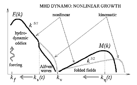
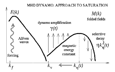
Figure 1: Sketches of the kinetic and magnetic energy spectra in the nonlinear regime. Left: the nonlinear-growth stage (section 3.2). During the kinematic stage, the velocity spectrum $E(k)$ is Kolmogorov, the magnetic spectrum $M(k)$ is peaked at $k_{\eta}\sim{Pr}^{1/2}k_{\nu}$. In the nonlinear-growth stage, the magnetic field is amplified by the eddies at the stretching scale $\ell_{\rm s}\sim k_{\rm s}^{-1}$. They are the eddies whose energy is equal to the total magnetic energy at any given time $t$. The motions with $k<k_{\rm s}(t)$ are still hydrodynamic, but those with $k>k_{\rm s}(t)$ are Alfvénic. As the magnetic energy grows, both $k_{\rm s}$ and $k_{\eta}$ decrease. Right: the approach to saturation (section 3.3). Selective decay eliminates high-$k$ modes, $k_{\eta}$ decreases, the stretching rate $\gamma\sim\eta k_{\eta}^{2}$ decreases accordingly, so the magnetic energy stays constant.

3.3 The approach to saturation

At this point, the hydrodynamic energy stirred up at the forcing scale is transfered directly into the small-scale folded magnetic field (i.e., in (2), $\gamma\sim k_{f}u_{0}$). As there are no scales in the system larger than $k_{f}^{-1}$, there can be no further growth of the magnetic energy. Indeed, the tension in the folds is now $\bi{B}\cdot\boldsymbol{\nabla}\bi{B}\sim k_{f}W$ and the force balance in (19) requires $\bi{B}\cdot\boldsymbol{\nabla}\bi{B}\sim\bi{u}\cdot\boldsymbol{\nabla}\bi{u}\sim k_{f}W_{0}$, so $W\sim W_{0}$. Note that setting $\rmd W/\rmd t=0$ in (2) gives $\gamma(t)=\eta k_{\rm rms}^{2}(t)$. This is a reflection of the fact that the resistive cutoff $k_{\eta}\sim k_{\rm rms}$ is now determined by the zero-sum balance between the field amplification (stretching) and the resistive dissipation:

$$\gamma(t)\sim\eta k_{\eta}^{2}(t).$$ (23)

However, at scales larger than the resistive cutoff, i.e., for $k<k_{\eta}$, the field-amplification rate $\gamma$ is larger than the resistive-dissipation rate $\eta k^{2}$ (figure 1, right panel). Since the total magnetic energy is not allowed to grow anymore, the growth of modes with $k<k_{\eta}$ must be compensated by the decrease in the value of $k_{\eta}$, i.e., by further selective decay of the high-$k$ modes. This, in turn, should lead to further decrease of $\gamma$ in accordance with the resistive balance (23). We shall see in section 4.4 that the evolution of the magnetic-energy spectrum in this regime is likely to be self-similar with $\gamma(t)\sim 1/t$ and $k_{\eta}(t)\sim(\eta t)^{-1/2}$.

Thus, we expect that this last stage of the nonlinear dynamo should be characterized by $\gamma$ dropping below the turnover rate $k_{f}u_{0}$ of the outer-scale eddies. Therefore, the rate of the energy transfer into the small-scale magnetic field decreases, as this channel of energy dissipation becomes inefficient. Instead, we expect the energy injected by the forcing to be increasingly diverted into the Alfvénic turbulence that is left throughout the inertial range in the wake of the suppression of the stretching motions.

3.4 The fully developed isotropic MHD turbulence

We saw in the preceding sections that $k_{\eta}$ decreases both in the nonlinear-growth stage and during the subsequent slower approach to saturation. It is very important to understand how far the decrease of $k_{\eta}$ can proceed. We recall that, in our arguments so far, we have disregarded the Alfvénic component of the turbulence. It is not, however, justified to do so after the small-scale magnetic energy reaches the velocity scales. Indeed, the decrease of $k_{\eta}(t)$ is basically a consequence of the balance between the field-amplification and the resistive-dissipation terms in the energy equation (2): as $\gamma(t)$ drops, so does $k_{\eta}(t)\sim k_{\rm rms}(t)$; once the characteristic scale of the small-scale fields reaches the viscous scale $k_{\nu}^{-1}$, the Alfvénic turbulence will start to affect $k_{\rm rms}$ in an essential way: since the waves are damped at the viscous scale, $k_{\rm rms}$ must stabilize at $k_{\rm rms}\sim k_{\nu}$. The resulting turbulent state features folded magnetic fields reversing directions at the viscous scale plus Alfvén waves in the inertial range propagating along the folds. There are then two possibilities: either (i) this represents the final steady state of the isotropic MHD turbulence, or (ii) further evolution will lead to unwinding of the folds and continued energy transfer to larger scales, so that the spectrum will eventually peak at the outer scale and have an Alfvénic power tail extending through the inertial range. The turbulence in the inertial range would in the latter case be of the usual Alfvén-wave kind [27, 28, 29], where the large-scale magnetic fluctuations provide a mean field along which the inertial-range Alfvén waves propagate. A generic MHD turbulent steady state would thus emerge at the end of the nonlinear-dynamo evolution. This dichotomy cannot be resolved at the level of the present model and requires further study. However, in either case, $k_{\rm rms}\sim k_{\nu}$, so the statistical steady state of the fully developed isotropic MHD turbulence is characterized by the equalization of the resistive and viscous scales.

The time scale at which such an equalization is brought about is the resistive time associated with the viscous scale of the turbulence: $t_{\eta}(k_{\nu})\sim\left(\eta k_{\nu}^{2}\right)^{-1}$. We immediately notice that, in order for the slow approach to saturation described in section 3.3 to be realizable, this time scale must be longer than the turnover time of the outer-scale eddies: $t_{\eta}(k_{\nu})\gg t_{0}$, which requires ${Pr}\gg{Re}^{1/2}$. In other words, the resistive scale at the end of the nonlinear-growth stage must still be smaller than the viscous scale: $k_{\eta}(t_{0})/k_{\nu}\sim{Pr}^{1/2}{Re}^{-1/4}\gg 1$. This constitutes the “true large-${Pr}$ regime,” which is the one relevant for astrophysical plasmas (thus, in the interstellar medium, ${Re}\sim 10^{4}$, ${Pr}\sim 10^{14}$). In this regime, the magnetic energy saturates at the equipartition level, $W\sim W_{0}$. From the energy balance (2), we get an estimate of the amount of turbulent power that is still dissipated resistively: $\chi\epsilon\sim\gamma W\sim\eta k_{\nu}^{2}W_{0}\sim\epsilon\,{Re}^{1/2}{Pr}^{-1}$. Thus, $\chi\ll 1$, i.e., most of the injected power now goes into the Alfvénic motions (which are dissipated viscously).

The other possibility is ${Pr}\lesssim{Re}^{1/2}$. In this case, the nonlinear-growth stage described in section 3.2 is curtailed with magnetic energy at a subequipartition value:

$$W\sim{t_{\eta}(k_{\nu})\over t_{0}}\,W_{0}\sim{{Pr}\over\sqrt{{Re}}}\,W_{0},$$ (24)

and resistivity continuing to take a significant ($\chi$ is order one) part in the dissipation of the turbulent energy. If no further evolution takes place [possibility (i) above], (24) gives an estimate of the saturation energy of the magnetic component of the turbulence. This regime is characterized by Prandtl numbers which may still be much larger than unity, but are not large enough to capture all of the physics of large-${Pr}$ dynamo. Most of the extant numerical simulations appear to be in this regime (see section 5).

We should now like to examine the implications of the proposed scenario in a somewhat more quantitative fashion, assuming from now on ${Pr}\gg{Re}^{1/2}\gg 1$. A busy reader with no time for these slow-paced developments may skip to section 5.

4 The Fokker–Planck model of the dynamo

4.1 Formulation of the model

The expression (22) suggests a way to build up the phenomenological picture just laid out into a semiquantitative model of the evolution of the magnetic spectrum throughout the nonlinear regime. Let us keep the general form of equation (5), but replace ${\bar{\gamma}}$ by a time-dependent function $\gamma(t)$, for which we stipulate the following ad hoc expression:

$$\gamma(t)=c_{1}\left[\int_{0}^{k_{\rm s}(t)}\rmd k\,k^{2}E(k)\right]^{1/2},\qquad c_{2}\int_{k_{\rm s}(t)}^{\infty}\rmd k\,E(k)=W(t),$$ (25)

where $c_{1}$ and $c_{2}$ are some numerical constants of order unity, $E(k)$ is the hydrodynamic energy spectrum in the absence of magnetic field, $k_{\rm s}(t)$ is defined by the second expression in (25), and $W(t)$ is the total magnetic energy at time $t$. The Fokker–Planck model we propose for the nonlinear evolution of the magnetic spectrum is then

$$\partial_{t}M={\gamma(t)\over 5}\left(k^{2}{\partial^{2}M\over\partial k^{2}}-2k{\partial M\over\partial k}+6M\right)-2\eta k^{2}M.$$ (26)

We now assume the following crude model profile of the hydrodynamic energy spectrum of the Kolmogorov turbulence in the absence of magnetic field:

$$E(k)=\cases{C_{\rm K}\epsilon^{2/3}k^{-5/3}&for $k\in[k_{f},k_{\nu}]$,\\ 0&elsewhere,\\ }$$ (27)

where $C_{\rm K}\simeq 1.5$ is the Kolmogorov constant. The value of $k_{\nu}$ is set to enforce consistency of the model profile (27) with the exact relation $\epsilon=2\nu\int_{0}^{\infty}\rmd k\,k^{2}E(k)$:

$$k_{\nu}=k_{f}\left(1+{\epsilon^{1/3}\over(3/2)C_{\rm K}\nu k_{f}^{4/3}}\right)^{3/4}\sim{Re}^{3/4}k_{f}.$$ (28)

Using (27), it is straightforward to derive from (25)

$$\gamma(t)={\bar{\gamma}}\left[1-{1\over\left(1+W_{0}/W_{\nu}\right)^{2}}\right]^{-1/2}\left[{1\over\left(1+W(t)/W_{\nu}\right)^{2}}-{1\over\left(1+W_{0}/W_{\nu}\right)^{2}}\right]^{1/2},$$ (29)

where $W_{\nu}={3\over 2}\,c_{2}C_{\rm K}\epsilon^{2/3}k_{\nu}^{-2/3}$ and $W_{0}=c_{2}\int_{0}^{\infty}\rmd k\,E(k)$ are of the order of the energies of the viscous- and of the outer-scale eddies, respectively. Here, ${\bar{\gamma}}=c_{1}(\epsilon/2\nu)^{1/2}$ follows from evaluating (25) for $W\to 0$, $k_{\rm s}=k_{\nu}$. Note that

$${W_{0}\over W_{\nu}}=\left({k_{\nu}\over k_{f}}\right)^{2/3}-1\sim{Re}^{1/2}\gg 1.$$ (30)

The kinematic regime $\gamma(t)\simeq{\bar{\gamma}}$ (section 2), the nonlinear-growth regime (22) (section 3.2), and the long-time asymptotic $\gamma(t)\to 0$ (section 3.3) are all contained in the model expression (29).

In the above formulae, $E(k)$ is the hydrodynamic turbulence spectrum in the absence of the magnetic field, and we have effectively assumed that, at each time $t$ during the evolution of the dynamo, $E(k)$ remains unaffected by the magnetic fields at $k<k_{\rm s}(t)$. As was explained in section 3.2, in the suppressed part of the inertial range $k>k_{\rm s}(t)$, Alfvénic turbulence is excited, which draws a finite fraction of the turbulent power and, indeed, in the long run, supplants the small-scale magnetic fields as the main energy-dissipation channel (see section 3.4). This part of the picture is not included in our Fokker–Planck model (26). We believe that it can be considered independently of the evolution of the small-scale magnetic-energy spectrum as long as the bulk of the magnetic energy stays below the viscous scale (see sections 3.4 and 4.5).

4.2 Self-similar solutions

The Fokker–Planck model (26) leads to the emergence of two distinct intermediate regimes where the magnetic-energy spectrum evolves in a self-similar fashion. In both regimes, the bulk of the magnetic energy moves from small to larger scales. We stress that the asymptotic self-similar solutions presented below are not sensitive to the particular form (29) of $\gamma(t)$. The essential features are those discussed in sections 3.2 and 3.3. The expression (29) will only be used to validate our solutions numerically.

Let us now study equation (26). We notice that, if $\gamma(t)$ can be represented as

$$\gamma(t)={\alpha\over t},$$ (31)

where $\alpha$ is a numerical constant, equation (26) admits a self-similar solution

$$M(t,k)={W(t)\over k_{\eta}(t)}\,\Phi(\xi),\qquad\xi=k/k_{\eta}(t),\qquad\int_{0}^{\infty}\rmd\xi\,\Phi(\xi)=1,$$ (32)

$$k_{\eta}(t)=\left[\gamma(t)/10\eta\right]^{1/2}=\left(\alpha/10\eta t\right)^{1/2},$$ (33)

$$W(t)=Ct^{\mu},$$ (34)

where the function $\Phi(\xi)$ satisfies

$$\xi^{2}\Phi^{\prime\prime}-\left(2+{5\over 2}\,\alpha^{-1}\right)\xi\Phi^{\prime}+\left(6-5\,{2\mu+1\over 2}\,\alpha^{-1}\right)\Phi-\xi^{2}\Phi=0.$$ (35)

Clearly, for $\gamma(t)\propto 1/t$, the appearance of self-similarity is inevitable on dimensional grounds because there is no fixed time scale in the problem in this case. The parameters $C$ and $\mu$ in (34) must be determined from the assumptions about the physics of the problem. The value of $\alpha$ is fixed by the solvability of equation (35).

4.3 The first self-similar regime: nonlinear growth

In section 3.2, we argued that $W(t)$ should grow linearly with time during the intermediate stage of the nonlinear dynamo when the magnetic back reaction gradually eliminates the stretching component of the inertial-range eddies. Thus, (34) should hold with $\mu=1$. Then, by virtue of (22), $\gamma(t)$ has the form (31) required for the self-similar solution to exist. The model expression (29) correctly reproduces this regime: substituting (31) into (29), we get

$$W(t)\simeq\alpha^{-1}{\bar{\gamma}}W_{\nu}t\simeq{\chi\epsilon\over 2\alpha}\,t,\qquad{\bar{\gamma}}^{-1}\ll t\ll{\bar{\gamma}}^{-1}{W_{0}\over W_{\nu}}\sim{\bar{\gamma}}^{-1}{Re}^{1/2}\sim t_{0}.$$ (36)

Comparing the above asymptotic with equation (21), we note that $1/2\alpha$ can be interpreted as the fraction of the turbulent power received by the magnetic fields that actually contributes to the growth of their energy. The rest is dissipated resistively. The upper time limit $t_{0}$ for this regime is the turnover time of the outer-scale eddies.

In order to determine the value of $\alpha$, we have to solve the equation (35) with $\mu=1$ and enforce the right boundary conditions. This is an eigenvalue problem very similar to that which we considered in section 2.4. The solution is again expressible in terms of the Macdonald function:

$$\Phi(\xi)={\rm const}\,\xi^{\sigma(\alpha)}K_{\nu(\alpha)}(\xi),\qquad\sigma(\alpha)={3\over 2}+{5\over 4}\,\alpha^{-1},$$ (37)

$$\nu(\alpha)={5\over 4}\left({1\over\alpha}-{1\over\alpha_{+}}\right)^{1/2}\left({1\over\alpha}-{1\over\alpha_{-}}\right)^{1/2},\qquad{1\over\alpha_{\pm}}={2\over 5}\left(\pm 4\sqrt{6}-9\right).$$ (38)

It is now necessary to implement the boundary condition at small $k$. Again, we should like to pick some finite IR cutoff $k_{*}$ and to impose the zero-flux condition (14) (see discussion in section 4.5 on the choice of $k_{*}$). However, strictly speaking, introducing the new dimensional parameter $k_{*}$ breaks the self-similarity of the problem: instead of (32), we must now write

$$M(t,k)={W(t)\over k_{\eta}(t)}\,\Phi(\xi,\xi_{*}),\qquad\int_{\xi_{*}}^{\infty}\rmd\xi\,\Phi(\xi,\xi_{*})=1,$$ (39)

where $\xi_{*}=k_{*}/k_{\eta}(t)=k_{*}(10\eta\alpha^{-1}t)^{1/2}$ is a new time-dependent dimensionless variable. Since the non-self-similar solution (39) has a self-similar asymptotic when $\xi_{*}\to 0$, we can still use (37), provided $\xi_{*}\ll 1$. This solution remains valid as long as $t\ll\alpha t_{\eta}$, where $t_{\eta}=(10\eta k_{*}^{2})^{-1}$ is the resistive time associated with the IR cutoff $k_{*}$. In large-${Pr}$ media, this is usually longer than the nonlinear-growth regime itself lasts according to (36) (see sections 3.4 and 4.5 though).

Figure 2: Evolution of $W(t)$ and $k_{\rm rms}(t)$ in a numerical solution of equation (26). In order to highlight scalings, an extreme asymptotic regime is considered in which ${Re}\sim 10^{7}$ and ${Pr}=10^{12}$. Left panel: time evolution of the quantity $\lambda(t)=\left[\gamma(t)\right]^{-1}{\rmd\over\rmd t}\ln W(t)$, which clearly exhibits all four asymptotic regimes of the dynamo: kinematic diffusion-free ($\lambda=2$, section 2.3), kinematic resistive ($\lambda=3/4$, section 2.4), nonlinear growth/first self-similar ($\lambda=\alpha^{-1}$, sections 3.2 and 4.3) and approach to saturation/second self-similar ($\lambda\propto t^{-2}$, sections 3.3 and 4.4). Right panel: corresponding time histories of $W(t)$ and $k_{\rm rms}(t)$ normalized by $W_{0}$ and $k_{\eta}^{\rm(kin)}$, respectively. Most of the exponential growth of $W(t)$ during the kinematic stage is not shown in order to resolve the nonlinear stages. The steady state (section 4.5), where the Fokker–Planck model (26) is not strictly valid, is not displayed either.

The zero-flux boundary condition for the self-similar solution (32) has the form (14) with $\xi_{*}=k_{*}/k_{\eta}(t)$. Substituting (37) into (14), we get the following equation for $\alpha$:

$$\left[\nu(\alpha)+\sigma(\alpha)-4\right]K_{\nu(\alpha)}(\xi_{*})-\xi_{*}K_{\nu(\alpha)+1}(\xi_{*})=0.$$ (40)

As explained above, this equation must be considered in the limit $\xi_{*}\ll 1$ and the resulting $\alpha$ must remain finite as $\xi_{*}\to 0$. Again there are no solutions with real $\nu(\alpha)$. For imaginary $\nu(\alpha)=\rmi{\tilde{\nu}}(\alpha)$, the requirement that the spectrum should have no nodes to the right of $\xi_{*}\ll 1$ again implies ${\tilde{\nu}}(\alpha)\ll 1$, and we get

$$K_{\rmi{\tilde{\nu}}(\alpha)}(\xi_{*})\simeq-{1\over{\tilde{\nu}}(\alpha)}\,\sin\left[{\tilde{\nu}}(\alpha)\ln(\xi_{*}/2)\right]=0,\qquad{\tilde{\nu}}(\alpha)\simeq 5^{1/2}6^{1/4}\left({1\over\alpha_{+}}-{1\over\alpha}\right)^{1/2}.$$ (41)

The solution is (see figure 2)

$$\alpha^{-1}\simeq\alpha^{-1}_{+}-{\pi^{2}\over 5\sqrt{6}\left[\ln(\xi_{*}/2)\right]^{2}}\simeq 0.32-\Or\left({1\over\ln^{2}(t/t_{\eta})}\right).$$ (42)

Since $t\ll t_{\eta}$, the spectral profile is well described by (37) with $\nu(\alpha)=0$ and $\sigma(\alpha)\simeq 1.9$.

Thus, in the first self-similar stage, the scale-by-scale suppression of the inertial-range eddies leads to gradual renormalization of the resistive cutoff $k_{\eta}(t)$, which is moving leftwards as $(\eta t)^{-1/2}$ in agreement with the estimate in section 3.2 (see figures 2, 3). The turbulent power arriving into the smallest unsuppressed eddies is (partially) transfered into the small-scale magnetic fields. The fraction $1/2\alpha$ ($\sim 16\%$) of it contributes to the linear-in-time growth of the total magnetic energy, while the rest is dissipated resistively. Since this stage of the dynamo lasts up to $t_{0}\sim{\bar{\gamma}}^{-1}{Re}^{1/2}$, we recover the physical estimates made in section 3.2: $W(t_{0})\sim{Re}^{1/2}W_{\nu}\sim W_{0}$ and $k_{\eta}(t_{0})\sim{Re}^{-1/4}k_{\eta}^{\rm(kin)}\sim\left({Re}\,{Pr}\right)^{1/2}k_{f}$.

Figure 3: Evolution of $M(t,k)$ in a numerical solution of equation (26). This is the same run as in figure 2. The spectra are normalized by $W(t)$.

Remark on the elongation of the folds. In section 3.2, we assumed the growth of the effective stretching scale $\ell_{\rm s}(t)$ during the nonlinear-growth stage to be accompanied by simultaneous elongation of the folds, so that the parallel scale of the magnetic field (characteristic length of the folds) would always be $\ell_{\parallel}(t)\sim\ell_{\rm s}(t)$. This assumption can now be supported in the following way. Consider a straight segment of a field line of length $\ell_{\parallel}$. In the absence of resistivity, volume- and flux-conservation constraints in an incompressible flow imply $\ell_{\parallel}/B\sim{\rm const}$, so $\rmd\log\ell_{\parallel}/\rmd t=(1/2)\,\rmd\log W/\rmd t=\gamma(t)$. With resistivity included, the growth of the magnetic field is offset by resistive diffusion. As we showed above, this lowers the net amplification rate of the magnetic energy to $\alpha^{-1}\gamma(t)$ in the first self-similar regime. However, the length of the field line continues to grow at the rate $\gamma(t)$, so $\rmd\log\ell_{\parallel}/\rmd t=\alpha\,\rmd\log W/\rmd t$. Using the nonlinear balance (20) and Kolmogorov scaling for velocity gives $\rmd\log\ell_{\parallel}/\rmd\log\ell_{\rm s}=2\alpha/3\simeq 2$. By itself, this would indicate that $\ell_{\parallel}$ grows even faster than $\ell_{\rm s}$. However, a straight section of a field line remains straight during stretching only as long as it is still short compared to the stretching-eddy size. Once $\ell_{\parallel}$ grows to be comparable to $\ell_{\rm s}$, it is limited to $\ell_{\parallel}\sim\ell_{\rm s}$ by the curvature in the stretching eddies. The conclusion from this argument is that the length of the folds can quickly adjust to the changing stretching scale. Note that this conclusion does not depend on the precise value of $\alpha$: it is sufficient that $\alpha^{-1}\leq 2/3$.

4.4 The second self-similar regime: approach to saturation

Thus, after time $t_{0}\sim{\bar{\gamma}}^{-1}{Re}^{1/2}$, the energy of the small-scale magnetic fields is very close to the equipartition energy $W_{0}$. We observe that in this regime it is still possible to have a self-similar solution in the form (32): the energy is now (nearly) constant, so $\mu=0$ in (34). Accordingly, substituting (31) into (29), we find

$$W(t)\simeq W_{0}\left[1-{\alpha^{2}\over 2}\left({t_{0}\over t}\right)^{2}\right],\qquad t\gg t_{0}={\bar{\gamma}}^{-1}{W_{0}\over W_{\nu}}\sim{\bar{\gamma}}^{-1}{Re}^{1/2}.$$ (43)

We now set $\mu=0$ in (35) and proceed to solve the resulting eigenvalue problem in exactly the same way as we did in section 4.3. All the same formulae and considerations apply, except that the expressions for $\alpha_{\pm}$ in (38) and for ${\tilde{\nu}}(\alpha)$ in (41) are now as follows:

$${1\over\alpha_{\pm}}=2\left(\pm 2\sqrt{2/5}-1\right),\qquad{\tilde{\nu}}(\alpha)\simeq 5^{3/4}2^{-1/4}\left({1\over\alpha_{+}}-{1\over\alpha}\right)^{1/2}.$$ (44)

The new eigenvalue is

$$\alpha^{-1}\simeq\alpha^{-1}_{+}-{\pi^{2}\over 5\sqrt{5/2}\left[\ln(\xi_{*}/2)\right]^{2}}\simeq 0.53-\Or\left({1\over\ln^{2}(t/t_{\eta})}\right).$$ (45)

For $t\ll t_{\eta}$, the spectrum is given by (37) with $\nu(\alpha)=0$ and $\sigma(\alpha)\simeq 2.2$.

Thus, in the second self-similar stage, the magnetic energy is nearly constant, but the resistive cutoff $k_{\eta}(t)$ continues to decrease as $(\eta t)^{-1/2}$, so the magnetic energy is redistributed from small to larger scales (see figures 2, 3). This is a very slow process, but it can, in principle, go on for a very long time: until self-similarity is broken at $t\sim t_{\eta}=(10\eta k_{*}^{2})^{-1}$. Note that, according to (43), the magnetic energy changes sufficiently slowly to make the left-hand side of the energy equation (2) subdominant in comparison with the field-amplification and resistive-dissipation terms in the right-hand side. This is consistent with the physical argument of section 3.3.

4.5 Steady states at the equipartition energy and below

The self-similar solutions obtained above break down after a finite time $\sim t_{\eta}$ due to the presence of the finite IR cutoff $k_{*}$. Once the resistive cutoff $k_{\eta}$ becomes comparable to $k_{*}$, the system arrives at the final steady state. The validity of this state is questionable since our model was derived under the assumption that the magnetic fields were at smaller scales than the velocity field, i.e. $k_{\eta}\gg k_{\nu}$. Furthermore, the specifications of the steady-state solution that the model yields clearly will have an order-one dependence on the value of the IR cutoff $k_{*}$, on the type of the boundary condition imposed, and on the form of the expression (29). However, we proceed to discuss this solution because it highlights several important issues that require further study.

In the steady state, $\gamma(t)\to\gamma(\infty)={\rm const}$, so the corresponding solution of equation (26) is simply the $\lambda=0$ eigenmode of the kinematic equation (5) with ${\bar{\gamma}}$ replaced by $\gamma(\infty)$: using equations (11) and (13), we get

$$M(k)={\rm const}\,\xi^{3/2}K_{i\sqrt{15}/2}(\xi),\qquad\xi=k/k_{\eta}(\infty),\qquad k_{\eta}(\infty)=\left[\gamma(\infty)/10\eta\right]^{1/2}.$$ (46)

The value of $\gamma(\infty)$ must be determined from the boundary condition at $k_{*}$:

$$\xi_{*}K^{\prime}_{i\sqrt{15}/2}(\xi_{*})-{5\over 2}\,K_{i\sqrt{15}/2}(\xi_{*})=0,\qquad\xi_{*}=k_{*}/k_{\eta}(\infty).$$ (47)

This is an equation for $\xi_{*}$, whose value in turn determines $\gamma(\infty)=10\eta k_{*}^{2}/\xi_{*}^{2}$. We have to pick the largest root of (47) to ensure that the spectrum (46) has no nodes. This gives $\xi_{*}\simeq 0.59$, which is order one, as expected. Substituting $\gamma(\infty)$ into (29), we get the magnetic energy $W(\infty)$ in the steady state:

$${W(\infty)\over W_{0}}=\left(1+{W_{\nu}\over W_{0}}\right)\left\{\left[1+\left(\left(1+{W_{0}\over W_{\nu}}\right)^{2}-1\right){\gamma^{2}(\infty)\over{\bar{\gamma}}^{2}}\right]^{-1/2}-\left(1+{W_{0}\over W_{\nu}}\right)^{-1}\right\},$$ (48)

which, using $W_{0}/W_{\nu}\sim{Re}^{1/2}\gg 1$ and $\gamma(\infty)/{\bar{\gamma}}=10\eta k_{*}^{2}/{\bar{\gamma}}\xi_{*}^{2}\sim\bigl{(}k_{*}/k_{\eta}^{\rm(kin)}\bigr{)}^{2}\sim\left(k_{*}/k_{\nu}\right)^{2}{Pr}^{-1}$, can be rewritten as follows

$${W(\infty)\over W_{0}}\sim\left[1+\left({k_{*}\over k_{\nu}}\right)^{4}{{Re}\over{Pr}^{2}}\right]^{-1/2}-{Re}^{-1/2}.$$ (49)

What is the correct choice of $k_{*}$? Of course, as long as the characteristic scale of the field is much smaller than that of all fluid motions, stretching or Alfvénic, i.e., $k_{\eta}\gg k_{\nu}$, the precise value of $k_{*}$ does not affect the self-similar asymptotics of sections 4.3 and 4.4 in the leading order. What $k_{*}$ represents is the presence in the problem of a spatial scale which leads to the breakdown of self-similarity in the long run (after time $t_{\eta}$). As we explained in section 3.4, once the resistive and the viscous scales become comparable, the evolution of the small-scale fields cannot be separated from that of the inertial-range Alfvénic turbulence. Clearly, beyond this point, the evolution of the spectrum is not described by the self-similar solutions obtained in sections 4.3 and 4.4. If we set $k_{*}\sim k_{\nu}$, the end of the self-similar regime and the stabilization of $k_{\eta}$ at a value $\sim k_{\nu}$ are reflected by the steady-state solution of our Fokker–Planck model. Note that, with this choice of $k_{*}$, equation (49) correctly reproduces both $W(\infty)\sim W_{0}$ for ${Pr}\gg{Re}^{1/2}$ and the physical estimate (24) of the subequipartition saturation level for ${Pr}\ll{Re}^{1/2}$. We stress that, since the validity of the Fokker–Planck model itself breaks down together with the self-similarity, the specific functional form of its steady-state solution cannot be expected to have predictive value. The ensuing regime is controlled by the interaction between the folded fields and the Alfvén waves and is left for future study.

5 Discussion

We have presented a physical scenario of the evolution of the nonlinear large-${Pr}$ dynamo according to which a magnetic-energy spectrum concentrated at velocity scales does emerge, but the time scale for it is resistive, not dynamical: the resistive scale approaches the viscous scale after $t_{\eta}\sim\left(\eta k_{\nu}^{2}\right)^{-1}$. In the interstellar medium, the Spitzer [42] value of the magnetic diffusivity is $\eta\sim 10^{7}~{}{\rm cm}^{2}/{\rm s}$, $k_{\nu}\sim 10^{-16}~{}{\rm cm}^{-1}$ [8], so $t_{\eta}\sim 10^{17}$ years, which exceeds the age of the Universe by 7 orders of magnitude! The conclusion is that this mechanism cannot be invoked as a workable feature of the galactic dynamo — at least not if the dissipation of the magnetic field is controlled by the Spitzer magnetic diffusivity.

The statistically steady solutions discussed in section 3.4 represent the possible long-time asymptotic states of the fully developed isotropic large-${Pr}$ MHD turbulence. Since the approach to these states is controlled by the resistive time scale associated with the velocity spatial scales, they have practically no relevance for astrophysical plasmas, which have large ${Re}$ and huge ${Pr}$. Studying these states may, therefore, appear to be a purely academic exercise in fundamental turbulence theory. While the importance of such pursuits ought never to be underestimated, we should like to point out another, more practical angle from which our results could be viewed. The enormous scale separations so often encountered in astrophysical objects are not accessible in the turbulence simulations that constitute the state of the art on Earth, so one usually has to be satisfied with only very modest ${Re}$ and ${Pr}$. Most of the numerical studies of the small-scale dynamo have so far adopted the strategy of resolving a reasonable hydrodynamic inertial range while only allowing for Prandtl numbers of at most order 10 [20, 21, 24, 25, 26, 43]. In this context, our steady-state solution and formula (48) point to an important possibility. When the scale separations in the problem are not very large, the system may converge to a steady state with a subequipartition magnetic energy $W(\infty)<W_{0}$. Subequipartion saturated states have indeed been reported in the numerical experiments cited above. Since the condition for the true asymptotic regime is ${Pr}\gg{Re}^{1/2}$ (section 3.4), numerical experiments with very high resolution are required to adequately study the large-${Pr}$ MHD turbulence.

In conclusion, we list some of the unresolved issues that require further study.

• The detailed mechanism of the flow suppression by the small-scale magnetic fields is a long-standing physical problem [44, 45, 46, 47]. In our model, we have conjectured the suppression of the shearing flows but allowed for oscillatory Alfvénic motions, that do not stretch the field (section 3.2). Strictly speaking, only the parallel component of the shear tensor $\boldsymbol{\nabla}\bi{u}$ must be suppressed in order to block the growth of the magnetic energy. The perpendicular components, if unaffected, could perhaps mix the field (without amplifying it) via a quasi-two-dimensional field-line-interchange mechanism and thus prevent any increase in the field’s characteristic scale. In fact, this seems to be the physics behind the recent numerical results on the large-${Pr}$ MHD turbulence with a fixed uniform mean field [48]. However, it is unclear to what extent such motions can remain quasi-two-dimensional and avoid twisting up the magnetic field, which would then resist further mixing — particularly, in our case of a folded field-line structure without an externally imposed mean field.

• Our physical picture of the final approach to saturation (section 3.3) is not based on a solid phenomenological argument such as that for the nonlinear-growth stage, and remains incompletely understood. Indeed, it remains to be proven definitively that the selective decay will continue after the small-scale magnetic energy reaches the energy of the outer-scale eddies. Due to resolution constraints discussed above, no numerical evidence of this regime is available as yet.

• Two possibilities for the long-time behaviour of the isotropic MHD turbulence were identified in section 3.4: saturation in the generic Alfvénic MHD turbulent state and saturation in a state where a significant amount of the magnetic energy remains tied up in the viscous-scale fields. Which one is realized depends on the way the small-scale folded fields interact with the inertial-range Alfvén-wave turbulence. We should like to observe that there is no numerical evidence available at present that would confirm that, the isotropic forced MHD turbulence without externally imposed mean field — at any Prandtl number — attains the Alfvénic state of scale-by-scale equipartition envisioned in Iroshnikov–Kraichnan [27, 28] or Goldreich–Sridhar [29] phenomenologies. In fact, medium-resolution numerical investigations [26] rather seem to support the final states with small-scale energy concentration even for ${Pr}=1$. This does not mean that the Alfvénic picture is incorrect per se. However, all existing phenomenologies of the Alfvénic turbulence depend on Kraichnan’s [28] assumption that the most energetic magnetic fields are those at the outer scale. This is automatically satisfied if a finite mean field is imposed externally [49, 50, 48]. However, it remains to be seen if such a distribution of energy is set up self-consistently when the turbulence is isotropic. The alternative identified here involves Alfvénic motions superimposed on small-scale folded fields.

• An extension of the MHD description itself that may change the properties of the small-scale magnetic turbulence is the incorporation of the Braginskii [51] tensor viscosity [52, 26, 53]. Even at magnetic energies small enough for the kinematic approximation to hold, the plasma is already well magnetized and the anisotropy of the viscous stress tensor leads to suppression of the velocity diffusion perpendicular to the local magnetic field [53]. This anisotropy is all the more important in view of the locally anisotropic (folding) structure of the magnetic field itself [3, 53].

• Another important extension is to allow compressible motions. The interstellar turbulence is sonic at the outer (supernova) scale but becomes subsonic and predominantly vortical in the inertial range (cf. [54, 55]). This is the commonly accepted justification for the use of incompressible MHD in the models of galactic dynamo. Of course, a certain amount of compressive motion is always present in the interstellar medium (as well as in other astrophysical plasmas), and it has been suggested in the literature that the compressibility of the motions and interactions between Alfvén waves and density inhomogeneities can be important in the description of turbulence (see, e.g., [56] and many recent references cited therein). The treatment of the kinematic-dynamo problem for a model compressible case can be found in [8, 3]. However, it remains to be understood whether and how weak compressibility affects the basic properties of the nonlinear dynamo.

It is a very old observation that any extension of the domain of one’s knowledge lengthens the perimeter along which this domain borders on the unknown. The perceptive reader must have realized that this work raises more questions than it gives definitive answers. We shall address these questions in our future investigations.

Appendix A Alfvén waves and folded fields

Defining $H^{ij}=B^{i}B^{j}$, we can write the MHD equations in the following tensor form:

$$\partial_{t}u^{i}+u^{k}\partial_{k}u^{i}=-\partial_{i}p+\partial_{k}H^{ik}+\nu\Delta u^{i}+f^{i},\qquad\partial_{i}u^{i}=0,$$ (50)

$$\partial_{t}H^{ij}+u^{k}\partial_{k}H^{ij}=H^{kj}\partial_{k}u^{i}+H^{ik}\partial_{k}u^{j}+\eta R^{ij},$$ (51)

where $\partial_{k}=\partial/\partial x^{k}$, and $R^{ij}=B^{i}\Delta B^{j}+B^{j}\Delta B^{i}$.

As we explained in section 3, the stretching and folding of the magnetic field by the turbulent eddies of scale $\ell_{\rm s}$ lead to the field becoming organized in folds of length $\ell_{\parallel}\sim\ell_{\rm s}$ with direction reversals within each fold at the scale $\ell_{\perp}\sim k_{\eta}^{-1}$ [3, 4]. Consider now some typical instance during the nonlinear stage of the dynamo when $k_{\nu}^{-1}\ll\ell_{\rm s}<k_{f}^{-1}$ (all stretching motions up to the scale $\ell_{\rm s}$ are suppressed). There is a clear scale separation in the problem: writing the magnetic-field tensor in the form $H^{ij}=b^{i}b^{j}B^{2}$, where $b^{i}=B^{i}/B$, we see that $B^{2}$ varies at scales $\ell_{\perp}\sim k_{\eta}^{-1}\ll k_{\nu}^{-1}$ while the tensor $b^{i}b^{j}$ varies at scales $\ell_{\parallel}\sim\ell_{\rm s}\gg k_{\nu}^{-1}$ ($b^{i}$ flips its sign at scale $\ell_{\perp}$, but this does not affect the tensor product $b^{i}b^{j}$). We can, therefore, average all fields over the subviscous scales: $\langle u^{i}\rangle_{\rm ss}=u^{i}$, $\langle H^{ij}\rangle_{\rm ss}=b^{i}b^{j}\langle B^{2}\rangle_{\rm ss}$. In the suppressed part of the inertial range, i.e. at scales $\ell$ such that $k_{\nu}^{-1}\ll\ell\ll\ell_{\rm s}$, the tensor $\langle H^{ij}\rangle_{\rm ss}=b^{i}b^{j}\langle B^{2}\rangle_{\rm ss}$ can be considered constant. Perturbing around this value and $u^{i}=0$, we find that equations (50)-(51) (without the dissipation terms) admit wave-like solutions with the dispersion relation

$$\omega=\pm k_{\parallel}v_{\rm A},\qquad k_{\parallel}=\sqrt{k_{i}k_{j}b^{i}b^{j}},\qquad v_{\rm A}=\sqrt{\langle B^{2}\rangle_{\rm ss}}.$$ (52)

These are Alfvén-like waves propagating along the folds of the direction-reversing magnetic fields, which are straight at scales below $\ell_{\rm s}$ (figure 4). These waves are a modification of the previously introduced magnetoelastic waves [57, 58] with account taken of the folding structure of the small-scale magnetic fields.

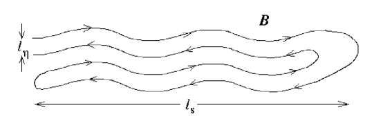
Figure 4: Alfvén waves propagate along folded magnetic fields.

In (52), we must have $\ell_{\rm s}^{-1}\ll k_{\parallel}\ll k_{\nu}$, so the frequency $\omega$ is larger than the characteristic time scale of the growth of the small-scale magnetic energy: $\omega=k_{\parallel}v_{\rm A}\gg v_{\rm A}/\ell_{\rm s}\sim W^{1/2}/\ell_{\rm s}\sim u_{\ell_{\rm s}}/\ell_{\rm s}\sim\gamma$. Since the resistive-dissipation rate of the small-scale fields is $\eta k_{\rm rms}^{2}\sim\gamma$ by virtue of (2), the Alfvén waves are mostly dissipated viscously via the MHD turbulent cascade. The velocity spectrum of this Alfvénic turbulence is subject to considerations similar to those arising in the Iroshnikov–Kraichnan [27, 28] or the Goldreich–Sridhar [29] phenomenologies. Further investigations of this and related issues will be published elsewhere.

References

References

- [1] Batchelor G K 1950 Proc. R. Soc.Ser. A 201 405
- [2] Ott E 1998 Phys. Plasmas 5 1636
- [3] Schekochihin A, Cowley S, Maron J and Malyshkin L 2002 Phys. Rev.E 65 016305
- [4] Schekochihin A A, Maron J L, Cowley S C and McWilliams J C 2002 Astrophys. J. 576 806
- [5] Batchelor G K 1959 J. Fluid Mech. 5 113
- [6] Kulsrud R M and Anderson S W 1992 Astrophys. J. 396 606
- [7] Kulsrud R M 1999 Annu. Rev. Astron. Astrophys. 37 37
- [8] Schekochihin A A, Boldyrev S A and Kulsrud R M 2002 Astrophys. J. 567 828
- [9] Balbus S A and Hawley J F 1998 Rev. Mod. Phys.70 1
- [10] Heinz S and Begelman M C 2000 Astrophys. J. 535 104
- [11] Kulsrud R M, Cen R, Ostriker J P and Ryu D 1997 Astrophys. J. 480 481
- [12] Malyshkin L 2001 Astrophys. J. 554 561
- [13] Narayan R and Medvedev M V 2001 Astrophys. J. 562 L129
- [14] Son D T 1999 Phys. Rev.D 59 063008
- [15] Christensson M, Hindmarsh M and Brandenburg A 2001 Phys. Rev.E 64 056405
- [16] Beck R 2000 Phil. Trans. R. Soc.A 358 777
- [17] Widrow L M 2002 Rev. Mod. Phys.74 775
- [18] Han J-L and Wielebinski R 2002 Chin. J. Astron. Astrophys. 2 293
- [19] Pouquet A, Frisch U and Léorat J 1976 J. Fluid Mech. 77 321
- [20] Meneguzzi M, Frisch U and Pouquet A 1981 Phys. Rev. Lett.47 1060
- [21] Kida S, Yanase S and Mizushima J 1991 Phys. Fluids A 3 457
- [22] Chandran B D G 1997 Astrophys. J. 485 148
- [23] Cho J and Vishniac E T 2000 Astrophys. J. 538 217
- [24] Brandenburg A 2001 Astrophys. J. 550 824
- [25] Chou H 2001 Astrophys. J. 556 1038
- [26] Maron J, Cowley S and McWilliams J 2003 Astrophys. J. submitted [Preprint astro-ph/0111008]
- [27] Iroshnikov P 1964 Sov. Astron. 7 566
- [28] Kraichnan R H 1965 Phys. Fluids 8 1385
- [29] Goldreich P and Sridhar S 1995 Astrophys. J. 438 763
- [30] Moffatt H K 1978 Magnetic Field Generation in Electrically Conducting Fluids (Cambridge: Cambridge University Press)
- [31] Blackman E G 2002 in Turbulence and Magnetic Fields in Astrophysics ed E Falgarone and T Passot (Berlin: Springer) in press [Preprint astro-ph/0205002]
- [32] Frisch U, Pouquet A, Léorat J and Mazure A 1975 J. Fluid Mech. 68 769
- [33] Cocke W J 1969 Phys. Fluids 12 2488
- [34] Orszag S A 1970 Phys. Fluids 13 2203
- [35] Kazantsev A P 1968 Sov. Phys.—JETP 26 1031
- [36] Kraichnan R H 1968 Phys. Fluids 11 945
- [37] Vainshtein S I 1980 Sov. Phys.—JETP 52 1099
- [38] Vainshtein S I 1982 Sov. Phys.—JETP 56 86
- [39] Gruzinov A, Cowley S and Sudan R 1996 Phys. Rev. Lett.77 4342
- [40] Schekochihin A A and Kulsrud R M 2001 Phys. Plasmas 8 4937
- [41] Orszag S A 1977, in Fluid Dynamics ed R Balian and J-L Peube (London: Gordon and Breach)
- [42] Spitzer L 1962 Physics of Fully Ionized Gases (New York: Interscience)
- [43] Brummell N H, Cattaneo F and Tobias S M 2001 Fluid Dyn. Res. 28 237
- [44] Cattaneo F, Hughes D W and Kim E 1996 Phys. Rev. Lett.76 2057
- [45] Zienicke E, Politano H and Pouquet A 1998 Phys. Rev. Lett.81 4640
- [46] Kim E 2000 Phys. Plasmas 7 1746
- [47] Nazarenko S V, Falkovich G E and Galtier S 2001 Phys. Rev.E 63 016408
- [48] Cho J, Lazarian A and Vishniac E T 2002 Astrophys. J. 566 L49
- [49] Maron J and Goldreich P 2001 Astrophys. J. 554 1175
- [50] Cho J, Lazarian A and Vishniac E T 2002 Astrophys. J. 564 291
- [51] Braginskii S I 1965 Rev. Plasma Phys. 1 205
- [52] Montgomery D 1992 J. Geophys. Res. A 97 4309
- [53] Malyshkin L and Kulsrud R 2002 Astrophys. J. 571 619
- [54] Balsara D and Pouquet A 1999 Phys. Plasmas 6 89
- [55] Lithwick Y and Goldreich P 2001 Astropys. J. 562 279
- [56] Tsiklauri D and Nakariakov V M 2002 Astron. Astrophys. 393 321
- [57] Gruzinov A V and Diamond P H 1996 Phys. Plasmas 3 1853
- [58] Chandran B D G 1997 Ph. D. Thesis (Princeton University)