The coronal topology of the rapidly rotating K0 dwarf, AB Doradus I. Using surface magnetic field maps to model the structure of the stellar corona

Abstract

We re-analyse spectropolarimetric data of AB Dor taken in 1996 December using a surface imaging code that can model the magnetic field of the star as a non-potential current-carrying magnetic field. We find that a non-potential field needs to be introduced in order to fit the dataset at this epoch. This non-potential component takes the form of a strong unidirectional azimuthal field of a similar strength to the radial field. This azimuthal field is concentrated around the boundary of the dark polar spot recovered at the surface of the star using Doppler imaging. As polarization signatures from the center of starspots are suppressed, it is unclear whether or not this non-potential component genuinely represents electric current at the unspotted surface or whether it results from the preferred detection of horizontal field in starspot penumbrae. This model contains 20% more energy than the corresponding potential field model at the surface. This amount of free energy drops to under 1% about 1 $\mbox{R}_{*}$ above the photosphere.

We use these surface maps to model the coronal structure of the star. The mixed radial polarities at the pole in the surface maps support closed coronal loops in the high latitude regions, indicating that a component of the X-ray emission may originate in this area. Assuming that the field remains closed out to 5 $\mbox{R}_{*}$  we find stable surfaces where prominences may form out to the observed distances using this coronal model.

1 Introduction

Doppler imaging allows us to map surface brightness distributions across the surfaces of rapidly rotating stars (Vogt & Penrod 1983). This technique has proven to be an important tool when studying activity in rapidly rotating solar-type stars. Spot maps show that, while sunspots tend to congregate between $\pm 30$^∘ latitude, spot patterns on other cool stars are different. In rapid rotators, strong spot activity is often concentrated in polar or high-latitude regions (Strassmeier 1996). This difference to the solar pattern has been the subject of much debate in recent years. The presence of strong flux at high latitudes may be explained in terms of increased Coriolis forces acting on flux tubes in the convective interior in rapidly rotating stars. These would lead to the emergence of flux tubes in high latitude regions (Schüssler & Solanki 1992). An alternative explanation for the polar spot phenomenon is that there are rings of alternating polarity at the pole (Schrijver & Title 2001). These are produced when increased flux is injected into solar-type models. Meridional flows transport this flux to the pole. As the flux injection rate is increased, flux cancellation occurs more slowly and results in strong flux gathering at the stellar pole.

In general, these dark starspots are assumed to mark the regions where the strongest magnetic flux is concentrated. However, it is likely that smaller spots exist below our resolution limit that we cannot reconstruct. Semel (1989) proposed applying standard Doppler imaging principles to circularly polarized spectra in order to detect magnetic fields on the surfaces of rapidly rotating stars. This technique is called Zeeman Doppler imaging (ZDI). Brown et al. (1991) first developed a code that employed maximum entropy techniques to enable the mapping of magnetic fields on the stellar photospheres. This method has since been applied to three rapidly rotating systems: the RS CVn binary, HR1099 (K1IV+G5V); the K0 dwarfs; AB Dor and LQ Hya (Donati & Collier Cameron 1997, Donati 1999). The technique is not very sensitive to magnetic fields in spotted regions, but the resulting maps typically show the presence of strong magnetic field even in relatively unspotted parts of the photosphere. A puzzling feature in these maps is that the radial and azimuthal field components across the surface are of about the same strength. This is very different to the solar case, where strong horizontal field is only found in sunspot penumbrae.

A criticism of ZDI has been that no relationship is assumed between the three components of the field vector thus enabling the reconstruction of physically unrealistic magnetic field distribution patterns such as monopoles at the stellar surface. Potential field configurations and their extrapolations have been used to model the global surface and coronal field of the Sun (Altschuler & Newkirk 1969). We show how the surface and coronal field of AB Dor can be modeled using the magnetic field maps obtained using an advanced version of ZDI. Hussain, Jardine & Collier Cameron (2001) describe a technique that introduces a relationship between the different components of the surface magnetic field vector by assuming that the observed data can be fitted using a potential field distribution. In this paper we extend this method to non-potential fields, i.e. we assume that the surface field can be modeled using a potential field plus a non-potential field component that represents the presence of electric currents. This method is similar to that described by Donati (2001).

The K0 dwarf, AB Doradus (HD 36705), is a relatively bright ($m_{V}\approx 7$) example of a class of very active cool stars that are just evolving onto the main sequence. Its distance has been measured to be 15pc using HIPPARCOS and VLBI interferometry and its age is estimated to be between 20 to 30 Myr (Guirado et al. 1997, Collier Cameron & Foing 1997). It rotates at roughly 50 times the solar rate, $P_{\mbox{rot}}=0.51479$ d (Pakull 1981). Its surface is covered with large cool starspots as indicated by rotational modulation of its photometric light curve (Rucinski 1985). AB Dor also displays strong X-ray variability on all timescales (Kürster et al. 1997). Long-term photometry indicates that the star was at its brightest in the first epoch of observation in 1978, it then decreased down to a minimum level in 1988 and has since been increasing steadily, most recently plateauing out to roughly the same $m_{V}$ level as 1978. This may be evidence of a solar-type activity cycle with the starspot coverage increasing and decreasing with a period of 22-23 years (Amado 2001).

Doppler images of this star have revealed the presence of a polar spot that has been consistently present since 1992 (Collier Cameron & Unruh 1994, Collier Cameron 1995, Donati & Collier Cameron 1997, Donati et al. 1999). The only image of AB Dor that does not display this polar feature was obtained using data taken in 1989 (Kürster, Schmitt & Cutispoto 1994), the star was at its minimum brightness level at this epoch and hence at its most spotted (Amado 2001). Hence this feature may be associated in some way with a stellar activity cycle. This polar spot should be associated with strong magnetic field if the solar stellar analogy applies. Lower-latitude spots are also recovered in Doppler maps but are found to be much less stable.

ZDI studies of AB Dor carried out annually since 1995 reveal magnetic field maps with strong field in even relatively unspotted parts of the photosphere. The strong unidirectional azimuthal flux recovered near the pole in maps obtained in successive years provides a puzzling non-solar pattern (Donati & Collier Cameron 1997, Donati et al. 1999, Hussain 2000). We re-analyse the best sampled dataset using a code that introduces a relationship between all three field components, and use this analysis to evaluate if this band of azimuthal flux is still present. These new surface maps are extrapolated to model the structure of the corona. This coronal topology is used to evaluate general properties of the stellar corona. The model is also used to compute sheet-like surfaces of stable mechanical equilibria taking the rotation of the star into account (Jardine et al. 2001). These are sites where the prominences are likely to form. We use these coronal magnetic field models to model the temperatures and densities expected in the corona of AB Dor in paper II (van Ballegooijen & Hussain 2002).

2 Magnetic field mapping

The basic principles behind the technique of Zeeman Doppler imaging (ZDI) are presented here (Semel 1989; Donati & Coller Cameron 1997). Circularly polarized spectra, “Stokes V spectra”, are sensitive to the line-of-sight components of the magnetic field. In the case of high resolution spectra from rapidly rotating stars the circularly polarized contributions from different regions of the visible stellar disk are separated in velocity-space. As the star rotates, a time series of circularly polarized spectra allow us to pinpoint the locations of magnetic field regions. High latitude magnetic field areas produce distortions that are confined to the centre of the line profile while low-latitude magnetic field distortions move out into the wings of the profile.

Stokes V spectra are sensitive to the longitudinal component of the field. Within the weak field regime (applicable to magnetic field strengths under 1kG) the amplitude of the signature scales with surface area covered by the magnetic field, and with field strength. Different field orientations produce distinctive signatures in dynamic spectra. Hence a time-series of spectra allows us to ascertain both the size, strength and the orientation of the magnetic region (Donati & Brown 1997).

This technique has been used to derive surface magnetic field maps for the K0 dwarves AB Dor, LQ Hya and the active G dwarf in the RS CVn binary system HR1099 (Donati & Coller Cameron 1997; Donati et al. 1999; Donati 1999). The magnetic field has been reconstructed assuming no interdependence between the radial, azimuthal and meridional field maps. This can lead to monopoles and other physically unrealistic magnetic field distributions. In the case of high inclination stars like AB Dor ($i=60^{\circ}$), the circularly polarized signatures from radial and meridional magnetic field regions are very similar and thus lead to cross-talk (Donati & Brown 1997). By imposing a relationship between the different components of the magnetic field vector, we can compensate for limitations in ZDI caused by the lack of sensitivity of circularly polarized profiles to certain field orientations such as low-latitude meridional field vectors (Hussain, Jardine & Collier Cameron 2001).

We have developed an advanced version of ZDI that imposes a relationship between the three components of the vector field ${\bf B}({\bf r})$. The magnetic field is written as a linear combination of non-potential and potential fields:

$${\bf B}({\bf r})={\bf B}_{\rm np}({\bf r})-\nabla D,$$ (1)

where $\nabla\cdot{\bf B}_{\rm np}=0$ and $\nabla^{2}D=0$. A simple model for the non-potential field is used. First, we assume that the radial component of the non-potential field vanishes, $B_{{\rm np},r}=0$. This is true by definition at the stellar surface, but we assume here for simplicity that it is also true at larger heights. Since $\nabla\cdot{\bf B}_{\rm np}=0$, the tangential components can be written as:

$$B_{{\rm np},\theta}=\frac{1}{r\sin\theta}\frac{\partial F}{\partial\phi},~{}~{}~{}~{}~{}~{}B_{{\rm np},\phi}=-\frac{1}{r}\frac{\partial F}{\partial\theta},$$ (2)

where $F({\bf r})$ is a scalar. This implies that the field lines of the non-potential field are closed curves that lie on spherical shells ($r$ = constant, $F$ = constant). Second, we assume that the electric current density ${\bf j}({\bf r})$ is derived from a potential $Q({\bf r})$:

$$\frac{4\pi}{c}{\bf j}=\nabla\times{\bf B}_{\rm np}=-\nabla Q.$$ (3)

It follows that $\nabla^{2}Q=0$, so the distribution of electric currents in the corona is uniquely determined by the current density $j_{r}(R_{*},\theta,\phi)$ through the photosphere. Inserting equation (2) into equation (3), we find that $F$ can be written as $F\equiv r^{2}\partial C/\partial r$, where $C({\bf r})$ is a harmonic function ($\nabla^{2}C=0$) and $Q$ is given by

$$Q\equiv\frac{1}{\sin\theta}\frac{\partial}{\partial\theta}\left(\sin\theta\frac{\partial C}{\partial\theta}\right)+\frac{1}{\sin^{2}\theta}\frac{\partial^{2}C}{\partial\phi^{2}}=-\frac{\partial}{\partial r}\left(r^{2}\frac{\partial C}{\partial r}\right).$$ (4)

The above assumptions are rather arbitrary, but they are an improvement over the conventional ZDI method in that they allow us to reconstruct electric currents in addition to the potential field.

The magnetic field is extrapolated out to a source surface, $R_{s}$, beyond which the field is assumed to be radial (Schatten, Wilcox & Ness 1969). While this solution is not force-free it allows us to pinpoint the areas where the surface field distribution becomes non-potential while still allowing for the extrapolation of the field out to the corona. The magnetic field is expressed in terms of spherical harmonics:

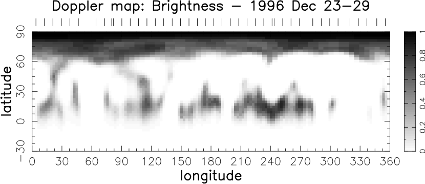
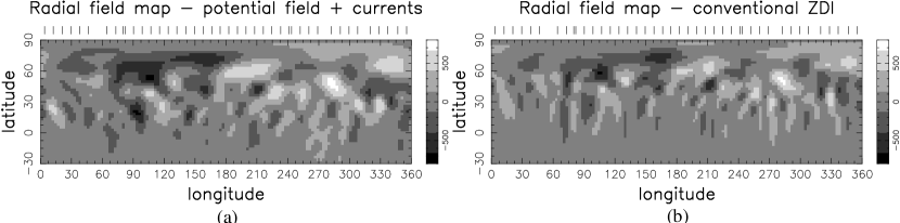
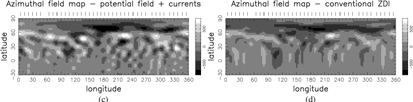
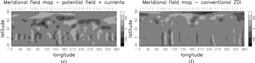
Figure 1: Surface brightness map for AB Dor in 1996 Dec 23-29. The greyscale for the brightness map represents spot occupancy for the star (1=complete spot coverage). The tick marks above each image indicate each phase of observation.

Figure 2: Magnetic field maps for AB Dor in 1996 Dec 23-29. The magnetic field maps in the left column were produced using the potential field and current prescription described here. The maps in the right column are those obtained using conventional ZDI (i.e. no assumed relationship between the three components of the magnetic field vector). All greyscales are the same (white/black represent $\pm$ 800G respectively). Both models fit the observed spectra to the same degree (reduced $\chi^{2}$=1.1).

Figure 3: The observed Stokes V intensity spectra from 1996 Dec 23-29 are shown by the error bars. The solid lines represent the spectral line profiles based on the non-potential magnetic field model (shown in the left-hand column of Fig.2). All spectra are plotted on the same intensity scale; the maximum polarization is $\pm 0.08$% of the continuum level. The phase of each observation is denoted at the bottom of each spectrum.

$$B_{r}(r,\theta,\phi) = \sum^{N}_{l=1}\sum^{l}_{m=-l}B_{lm}P_{lm}(\theta)f_{l}(r)e^{im\phi},$$ (5)

$$B_{\theta}(r,\theta,\phi) = -\sum^{N}_{l=1}\sum^{l}_{m=-l}[B_{lm}\frac{d}{d\theta}P_{lm}(\theta)g_{l}(r)$$ (6)

$$+(l+1)C_{lm}\frac{P_{lm}(\theta)}{\sin\theta}imr^{-(l+1)}]e^{im\phi},$$

$$B_{\phi}(r,\theta,\phi) = -\sum^{N}_{l=1}\sum^{l}_{m=-l}[B_{lm}\frac{P_{lm}(\theta)}{\sin\theta}img_{l}(r)$$ (7)

$$-(l+1)C_{lm}\frac{d}{d\theta}P_{lm}(\theta)r^{-(l+1)}]e^{im\phi}.$$

Here $\theta$ represents co-latitude; $\phi$ represents longitude; $B_{lm}$ represents the radial field at the stellar surface; $C_{lm}$ is the coefficient of the electric current; $P_{lm}(\theta)$ is the associated Legendre function at each latitude; the functions, $f_{l}(r)$ and $g_{l}(r)$ are given by (Nash, Sheeley & Wang 1988):

$$f_{l}(r)=\frac{(l+1)r^{-l-2}+lR_{s}^{-2l-1}r^{l-1}}{l+1+lR_{s}^{-2l-1}},$$

$$g_{l}(r)=\frac{r^{-l-2}-R_{s}^{-2l-1}r^{l-1}}{l+1+lR_{s}^{-2l-1}}.$$

We use $N=23$ as this corresponds to a spatial resolution of 2.5^∘ at the equator (i.e. the limit of the spectral resolution). The ZDI code maps different $B_{lm}$ and $C_{lm}$ configurations until the dataset is fitted. The radial, azimuthal and meridional field maps at the surface are then reconstructed using Eqns. (5), (6) and (7). The source surface, $R_{s}$ is initially set to 5 $\mbox{R}_{*}$ as prominence-type complexes are found to be supported out to these heights at this epoch (Donati et al. 1999). See Secn. 4 for a more detailed discussion of this parameter.

2.1 Weighting scheme

As several solutions can fit the observed spectral dataset to within any level of $\chi^{2}$, a regularising function is required to obtain a unique solution. We use maximum entropy in order to obtain the ’simplest’ possible image. We define the simplest image as the image that has the least number of nodes across the stellar surface while still fitting the observed dataset. Weights are assigned such that the image is biased towards the lowest order harmonics. See Hussain, Jardine & Collier Cameron (2001) for more discussion on the effect of different weighting schemes. The weighting scheme used here defines weights as follows:

$$\frac{1}{W(l,m)}=[(2|m|+1)(l-|m|+1)]^{2}.$$ (8)

Different schemes were tested and this one was chosen as it produced the quickest convergence to a unique solution.

2.2 Dataset

The spectroscopic observations used to obtain the magnetic field map for AB Dor were obtained as part of a long-term stellar activity monitoring programme over the week of 1996 December 23-29. The Semel polarimeter (Semel 1993) was mounted at the Cassegrain focus of the 3.9m Anglo-Australian Telescope and linked to the ucles spectrograph. For details of the instrumental setup and observing run, see Donati et al. (1997) and Donati & Collier Cameron (1997). The technique of least squares deconvolution (LSD) is used to improve the signal-to-noise ratio of the Stokes V profiles (Donati et al. 1999). It essentially cross-correlates thousands of selected line profiles with an appropriately weighted mask to produce a mean line profile with reduced noise.

The intrinsic line profile is assumed to remain constant across the entire visible stellar disc. The central wavelength and Landé factor of the mean LSD line profile is used to generate a look up table that contains the mean Stokes V profiles as a function of limb angle for a magnetic field at the equipartition strength (taken to be a maximum at 1.5 kG). See Hussain et al. (2000) for more detail on how these LSD profiles were produced. Data were combined from all four nights (1996 Dec. 23, 25, 27 and 29) in order to obtain as complete phase coverage as possible.

3 Surface magnetic field map of AB Dor

Initially the observed circularly polarized spectra were analysed using a code that just allowed for potential field solutions (Hussain, Jardine & Collier Cameron 2001). The observed differential rotation rate of the star, $\Omega(l)$, was taken into account when combining spectra taken over 1 week (i.e. 14 rotation cycles): $\Omega(l)=12.2434-0.0564\sin^{2}l$ rad  d^-1, where $l$ is the latitude on the star (Donati & Collier Cameron 1997, Donati et al. 1999). However, it was not possible to find a solution with a reduced $\chi^{2}<2$ for this dataset.

On allowing for an electric current component we find that this provides the additional freedom to fit the observed dataset to a reduced $\chi^{2}$ level of 1 (see Fig. 3). It should be noted that this is not a force-free solution. However, this method does have the advantage in that it does allow us to pinpoint the regions at which the field distribution departs from being purely potential, as well as enabling us to extrapolate the surface field out to the corona.

As AB Dor is inclined at $i=60$^∘ the magnetic field cannot be reconstructed reliably below a latitude, $l=-30$^∘. The high inclination angle means that the contribution of the meridional (N-S) field component to the circularly polarized profiles is suppressed and subject to cross-talk with the radial field component, especially at lower latitudes (Donati & Brown 1997). This may explain why the recovered meridional field is considerably weaker than either radial or azimuthal field components. There may be stronger meridional field at the stellar surface that we cannot recover using circularly polarized profiles alone. Once Stokes Q and U profiles can also be included in the reconstruction process it should be possible to improve the accuracy of the meridional field maps. Unfortunately at present it is not possible to obtain linear polarization signatures with sufficiently high S/N for this purpose.

The magnetic field analysis assumes that the intrinsic line depth across the stellar surface is uniform. This means that the spotted regions remain unaccounted for and the magnetic field at the surface is likely to be much stronger, particularly in the dark, spotted regions. This especially applies to the polar cap, where the dense spot coverage suppresses the contribution to the polarization signature from the entire region. It is possible that the strong azimuthal field that is recovered represents strong horizontal field in the penumbrae of the starspots and that more radial field at the surface is suppressed as it is located in the center of the spot umbrae. While the contribution from the meridional (N-S) field component to circularly polarized spectra is suppressed in the lower latitudes of high inclination stars (like AB Dor), the meridional field contribution should be strong in the polar region. The origin of the strong negative azimuthal field in the penumbrae of the polar region is still unclear.

3.1 Comparison with conventional ZDI

The maps shown in Fig. 2 are Cartesian projections of the stellar surface. The radial and azimuthal magnetic field maps in Fig. 2 show very similar distributions to those obtained using conventional ZDI (i.e. no assumed relationship between the components of the field vector). The radial field maps (Figs. 2a & b) differ only in the relative areas of the field that are reconstructed. These differences are not significant and can be affected by slight differences in the degree of fit that the images are pushed to (i.e. the level of agreement to the data as measured by $\chi^{2}$). Both the non-potential magnetic field model and the ZDI model fit the observed spectra to a reduced $\chi^{2}=1.1$. Fig. 3 shows the fits to the observed spectra from the non-potential magnetic field model. There is some difference between the two azimuthal field maps (Figs. 2c & d). In particular, in the conventional ZDI model there is an unbroken band of negative azimuthal field above a latitude of 60^∘  whereas in the non-potential field model some positive azimuthal field is also reconstructed near longitude 0^∘.

As with Doppler imaging, spectral signatures from low latitude features move through the line profile much more quickly than the signatures from higher latitude fields as the star rotates. This makes it harder to constrain the location of equatorial features. As the code preferentially produces images with as little structure as possible, it essentially weights against equatorial features which have large areas. Structure is pushed away from the equator and this results in the smearing effect seen in these maps. This smearing is particularly noticeable in the meridional field maps, where low-latitude spots are subject to cross-talk with the radial field maps in high inclination stars. The lack of constraints in the meridional field maps is also reflected in the differences between Figs.  2e & f.

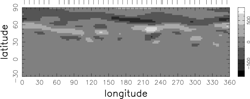
Figure 4: Non-potential component of azimuthal field for the same reconstruction as shown in Fig.2c. Greyscales and tick marks represent the strength of the magnetic field (in Gauss) and observation phases respectively (as in Fig. 2).

3.2 Azimuthal component

As mentioned above, these new maps do not show the same unbroken band of azimuthal field near the pole. While there is still strong negative azimuthal field in this region, the band is not complete and is even broken with a region of positive polarity near 0^∘ longitude (see Fig. 2c). Fig. 4 shows the contribution of the electric currents (the last term in Eqn. 7) to the azimuthal field. In this figure, there is some field around 50^∘ latitude but the strongest field is associated with the strong negative band of azimuthal field between 70^∘ and 80^∘ latitude.

Preliminary results obtained by carrying out a similar analysis on 1995 and 1998 datasets also suggest that the strong negative component may be increasing in strength with subsequent years. In the 1995 dataset, there is no need to invoke a non-potential component to fit the observed spectra within a reduced $\chi^{2}\approx 1$. What this non-potential component actually represents is unclear. As these maps are flux-censored in the spotted regions, it may be that the non-potential component exists only in certain parts of the penumbrae and not in others. The fraction of the penumbrae with azimuthal fields is apparently increasing with time. The origin of this magnetic shear in the penumbra of the polar spot is still unclear.

4 Coronal magnetic field

As described in Secn. 2 the magnetic field, B, can be written in terms of spherical harmonic functions and can be used to determine the radial dependence of the field. The resulting coronal magnetic field topology is shown in Fig. 5. The magnetic field is shown for two values of the source surface radius, $R_{s}$ [see Eqns.5-7].

Fast moving H$\alpha$ absorption transients have been reported in the optical spectra of this object at every epoch at which it has been observed (Robinson & Collier Cameron 1986, Collier Cameron et al. 1990). These transients can be explained in terms of the presence of slingshot-type prominence complexes forced into rigid corotation with the system. The rate of the transit of these cool (9000 K) clouds allow us to determine their axial distances from the stellar rotation axis. In 1996 December these prominences were found at various distances above the Keplerian corotation radius of the star ($R_{k}\approx 2.6$ $\mbox{R}_{*}$) up to 5 $\mbox{R}_{*}$ (Donati et al. 1999). This means that the magnetic field must be capable of supporting closed loop structures at these distances and so we initially set $R_{s}=5$ $\mbox{R}_{*}$ (see Fig.5a). However, in paper II we argue on the basis of the observed EUV emission from AB Dor that the gas pressure in coronal loops with heights beyond 1.7 $\mbox{R}_{*}$ would exceed the magnetic presure, hence the plasma in these loops cannot be magnetically contained. Therefore in Fig.5b we show a second model with the source surface located at $R_{s}=$1.7 $\mbox{R}_{*}$.

The mixed polarities in the surface radial field map allow closed loops to form over the polar region of the star. This indicates that plasma can be supported over the pole of the star, and that at least some of the observed coronal emission from AB Dor could originate here. This is indeed what is suggested by observations. For example, Maggio et al. (2000) report an observation of a compact flare ($H\approx 0.3$ $\mbox{R}_{*}$) which took a rotation period to decay and showed no evidence of self-eclipse. Furthermore, there is evidence from other active cool star systems, such as in the binaries 44i Boo and Algol. In the former case, a strong emission feature at $T\approx 8\times 10^{6}$ K indicating very dense, hot plasma confined close to the stellar surface. That this emission showed no sign of eclipse over a rotation cycle suggests that these hot loops may be located at the pole of the star (Brickhouse & Dupree 1998). A flare observed in Algol (B8 V + K2 IV) using BEPPOSAX originating on the K component was completely eclipsed by the hot star and allowed accurate determination of its physical characteristics. The analysis revealed that the flare’s maximum height was 0.6 $\mbox{R}_{*}$ and that it was located at the southern pole of the cool star component of the system, Algol B (Schmitt & Favata 1999).

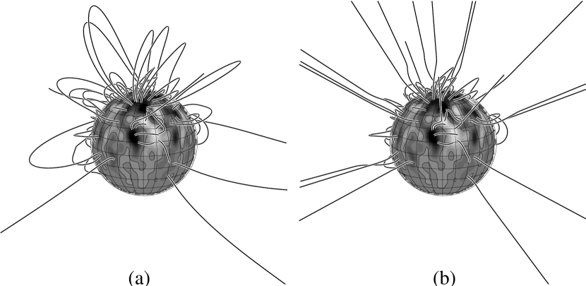
Figure 5: Coronal magnetic field of AB Dor for two values of the source surface radius: (a) $R_{s}=5$ $\mbox{R}_{*}$, and (b) 1.7 $\mbox{R}_{*}$.

5 H$\alpha$ prominences

As described in Secn.4, there is evidence for cool slingshot-type prominences formations lying well above the Keplerian co-rotation radius of AB Dor, at distances of up to 5 $\mbox{R}_{*}$ (Donati et al. 1999). Ferreira (2000) decribes how a prominence may be modeled in rapidly rotating stars if it is represented as an axisymmetric current sheet in a perfectly conducting plasma. An equilibrium can be found between the gravity, centrifugal and Lorentz forces acting on the current sheet. These prominences are most likely to form at stable points in the corona. Stable equilibria satisfy two conditions (Ferreira 2000):

• for equilibrium, the effective gravity component, $g_{\hbox{eff}}$, along a field line B must be zero and

• for a stable equilibrium, the location must be a minimum of the effective gravitational potential.

These stable points are also positions where the plasma pressure is a maximum along a field line. Jardine et al (2001) developed a general method to compute the locations of these stable points in arbitrary field configurations. We have improved their technique by solving numerically for positions of pressure maxima along field lines rather than interpolating from a grid of field vectors. This is more accurate close to the star where the field is complex and avoids the problem with the original method of a coarse grid leading to spurious stable points. Here we apply this method to the non-potential field model of AB Dor shown in Fig. 5a.

Our model of stable sheet-like surfaces are shown in Fig. 6. This plot shows that the main loci of equilibria where prominences could form starts at about the Keplerian co-rotation radius (2.6 $\mbox{R}_{*}$) and extends out to the source surface ($R_{s}=5$ $\mbox{R}_{*}$). Note that although closed loops form over the pole, there are no stable equilibria here as there is no centrifugal support. The prominences shown here would transit the stellar disk as the star rotates and could explain the observed H$\alpha$ absorption transients. The model shown in Fig. 6 would suggest that prominences can form above 2.5 $\mbox{R}_{*}$ up to the source surface, but that they should be confined to two small ranges of longitude (approximately $180^{\circ}$-$200^{\circ}$ and $350^{\circ}$-$20^{\circ}$). However, Donati et al. (1999) measure prominence-type complexes lying between 2.5-5 $\mbox{R}_{*}$ at almost all observed longitudes using this same dataset. Therefore the model with $R_{s}=5$ $\mbox{R}_{*}$ cannot explain the wide range of longitudes at which prominences are found to occur. In contrast, a model with lower source surface would produce many more polarity reversals. Therefore, a possible solution of the longitude problem is that $R_{s}=1.7$ $\mbox{R}_{*}$ and the prominences are located above the source surface at longitudes where the radial magnetic field changes sign (similar to the coronal streamers observed on the Sun). In this case the prominences are located in a nearly radial field and cannot be in static equilibrium. Further modeling is required to determine whether the observed H$\alpha$ prominences can be explained in this way.

A word of caution when comparing this model with observations is necessary here. The analysis of prominences using H$\alpha$ data carried out by Donati et al. (1999) suggests that coronal features evolve on a timescale of under 2 days and hence much more quickly than timescales of surface features (which are thought to have timescales on the order of 2 weeks or more). The coronal model that we have computed is based on surface maps that were obtained by combining data taken over one whole week. Observations would suggest that the coronal field or at least the component of the field that supports prominences is subject to considerable variability over the course of a week. This model also does not take the field in the starspots into account. The missing field is of unknown strength and polarity and, particularly, if the field in the high latitude spots is unipolar it will flatten the prominence sheet into an equatorial current sheet.

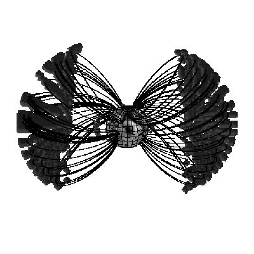
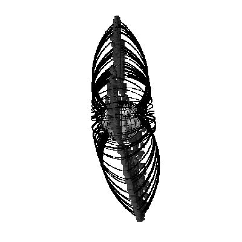
Figure 6: Locations of mechanical equilibria showing where prominence type complexes can be supported centrifugally. This model was computed using the coronal topology in Fig.5a (source surface, $R_{s}=5$ $\mbox{R}_{*}$). Phases 0.25 and 0.5 are pictured here.

6 Discussion

The magnetic field analysis of the stellar surface indicates that there is a strong non-potential field encircling the polar spot on AB Dor in 1996 December. This azimuthal field in located in the penumbra of the polar spot and its detection may be affected by the reduced visibility of the magnetic fields in the spotted regions. However, the observed azimuthal field appears to be real.

Schrijver & Title (2001) model the effect that the increased magnetic flux injected onto the surfaces of solar-type stars would have on subsequent flux patterns. They find that concentric bands of radial field with opposite polarity form near the pole of the star. This is a consequence of meridional transport of flux and the increased amount of flux dissipating on longer timescales. While our maps do not show this pattern, if there is strong flux of opposite polarities in the polar spot, meridional fields would connect the alternating bands of radial field. As the star rotates differentially, this horizontal field would be sheared in the azimuthal direction. Therefore, this model can in principle explain the origin of the azimuthal field.

Alternatively, there is preliminary evidence associating this azimuthal feature with the epoch of observation. First results suggest that the 1995 December images show no strong non-potential component and that 1998 January images have an even stronger non-potential component than required by the 1996 December dataset. Could this non-potential component be related to the stellar activity cycle? Does it switch direction over the course of the cycle? These are questions that analysis of subsequent datasets will answer. If this non-potential component is indeed real it is possible to evaluate the amount of magnetic energy available to power flares and coronal mass ejections. The amount of free energy integrated over the entire coronal volume is 14% of the potential-field energy. Fig. 7 shows how the ratio of non-potential and potential magnetic energy densities depends on height. The amount of extra energy drops off with height from 20% at the surface to well under 1% at the source surface height (5 $\mbox{R}_{*}$).

Analysis of subsequent datasets will reveal how typical the features recovered in this paper are and if they evolve from year to year. The method presented here promises to be an important tool in probing the dynamo activity of rapidly rotating cool stars.

Figure 7: The ratio of non-potential to potential magnetic field energy as a function of height. As this figure shows, the amount of free energy is greatest at the surface and drops quickly, levelling out to under 1% about 1 $\mbox{R}_{*}$ above the photosphere.

When modeling the coronal structure of the star it is necessary to define the point beyond which the field is open and radial. In the model presented in Fig. 6, this value has been set to 5 $\mbox{R}_{*}$ as suggested by the presence of prominences at these distances. This model would apply if these prominences fit the model of slingshot-type prominences. Observations suggest that prominences form out to 5 $\mbox{R}_{*}$, are stable over one rotation cycle but tend to have been ejected over a period of two days. This instability may reflect the inherent variability in the coronal field of AB Dor. Surface features recovered on AB Dor are, by contrast, stable on timescales of over a week.

If the source surface is at 1.7 $\mbox{R}_{*}$ as suggested by an analysis of the gas and magnetic pressures in AB Dor’s corona (see Paper II), the prominences are located beyond the source surface and their equilibrium and stability cannot be described in terms of potential field models. The magnetic field beyond the source surface is nearly radial with current sheets separating regions with opposite sign of $B_{r}$. According to this new model the prominences would be associated with these current sheets, but unlike in Fig. 6 they would not be in a state if magnetostatic equilibrium. Instead, the prominence plasma would slowly flow outward along the current sheets with velocity significantly less than the rotational velocity. This new model may explain the observation that prominences occur over a broad range of longitudes.

References

- (1)
- (2) Altschuler M., Newkirk Jr. G., 1969, Solar Phys., 9, 131
- (3)
- (4) Amado P., Cutispoto G., Lanza A., Rodonó M., 2001, in García López R., Rebolo R., Zapatero Osorio M., (eds.), 11th Cambridge Workshop on Cool Stars, Stellar Systems and the Sun. ASP Conference Series, San Francisco, Vol. 223, p.895
- (5)
- (6) Brickhouse N., Dupree A., 1998, ApJ, 502, 931
- (7)
- (8) Brown S.F., Donati J.-F., Rees D.E., Semel M., 1991, A&A, 250, 463
- (9)
- (10) Collier Cameron A., 1995, MNRAS, 275, 534
- (11)
- (12) Collier Cameron A., Foing B.H., 1997, Obs., 117, 218
- (13)
- (14) Collier Cameron A., Duncan D. K., Ehrenfreund P., Foing B. H., Kuntz K. D., Penston M. V., Robinson R. D., Soderblom D. R., 1990, MNRAS, 247, 415
- (15)
- (16) Collier Cameron A., Unruh Y.C., 1994, MNRAS, 269, 814
- (17)
- (18) Donati J.-F., Brown S. F., 1997, AA, 326, 1135
- (19)
- (20) Donati J.-F., Collier Cameron A., 1997, MNRAS, 291, 1
- (21)
- (22) Donati J.-F., Semel M., Carter B., Rees D. E., Collier Cameron A., 1997, MNRAS, 291, 658
- (23)
- (24) Donati J.-F., Collier Cameron A., Hussain G. A. J., Semel M., 1999, MNRAS, 302, 437
- (25)
- (26) Donati J.-F., 1999, MNRAS, 302, 457
- (27)
- (28) Donati J.-F., 2001, in: Boffin H., Steeghs D., Cuypers J. (eds.), First International Workshop on Astro-Tomography. Springer, Berlin (in press)
- (29)
- (30) Ferreira J., 2000, MNRAS, 316, 647
- (31)
- (32) Guirado J.C. et al. 1997, ApJ 490, 835
- (33)
- (34) Hussain G., Jardine M., Collier Cameron A., 2001, MNRAS, 322, 681
- (35)
- (36) Hussain G., Donati J.-F., Collier Cameron A., Barnes J., 2000, MNRAS, 318, 961
- (37)
- (38) Jardine M., Collier Cameron A., Donati J.-F., Pointer G. R., 2001, MNRAS, 324, 201
- (39)
- (40) Kürster M., Schmitt J., Cutispoto G., Dennerl K., 1997, A&A, 320, 831
- (41)
- (42) Kürster M., Schmitt J. H. M. M., Cutispoto G., 1994, A&A, 289, 899
- (43)
- (44) Maggio A., Pallavicini R., Reale F., Tagliaferri G., 2000, A&A, 356, 627
- (45)
- (46) Nash A.G. and Sheeley N.R., Jr. and Wang Y.-M., 1988, Solar Phys. 117, 359
- (47)
- (48) Pakull M. W., 1981, A&A, 104, 33
- (49)
- (50) Robinson R. D., Collier Cameron A., 1986, Proc. Astron. Soc. Aust., 6, 308
- (51)
- (52) Rosner R., Tucker W. H., Vaiana G. S., 1978, ApJ, 220, 643
- (53)
- (54) Rucinski S. M., 1985, MNRAS, 215, 591
- (55)
- (56) Schatten K.H, Wilcox J.M., Ness N.F., 1969, Solar Phys, 6, 442
- (57)
- (58) Schmitt J. H. M. M., Favata F., 1999, Nature, 401, 44
- (59)
- (60) Schrijver C., Title A., 2001, ApJ, 551, 1099
- (61)
- (62) Schüssler M., Solanki S. K., 1992, A&A, 264, L13
- (63)
- (64) Semel M., 1989, A&A, 225, 456
- (65)
- (66) Semel M., 1993, A&A, 278, 231
- (67)
- (68) Serio S., Peres G., Vaiana G. S., Golub L., Rosner R., 1981, ApJ, 243, 288
- (69)
- (70) Strassmeier K., 1996, in Strassmeier, K.G., Linsky, J.L., eds, IAU Symposium 176: Stellar Surface Structure. Kluwer, p. 289
- (71)
- (72) van Ballegooijen A., Cartledge N., Priest E., 1998, ApJ, 501, 866
- (73)
- (74) van Ballegooijen A., Hussain G., 2002, ApJ (in preparation)
- (75)
- (76) Vesecky J. F., Antiochos S. K., Underwood J. H., 1979, ApJ, 233, 987
- (77)
- (78) Vogt S. S., Penrod G. D., 1983, PASP, 95, 565
- (79)