A CLEAN-based Method for Deconvolving Interstellar Pulse Broadening from Radio Pulses

Abstract

Multipath propagation in the interstellar medium distorts radio pulses, an effect predominant for distant pulsars observed at low frequencies. Typically, broadened pulses are analyzed to determine the amount of propagation-induced pulse broadening, but with little interest in determining the undistorted pulse shapes. In this paper we develop and apply a method that recovers both the intrinsic pulse shape and the pulse broadening function that describes the scattering of an impulse. The method resembles the CLEAN algorithm used in synthesis imaging applications, although we search for the best pulse broadening function, and perform a true deconvolution to recover intrinsic pulse structre. As figures of merit to optimize the deconvolution, we use the positivity and symmetry of the deconvolved result along with the mean square residual and the number of points below a given threshold. Our method makes no prior assumptions about the intrinsic pulse shape and can be used for a range of scattering functions for the interstellar medium. It can therefore be applied to a wider variety of measured pulse shapes and degrees of scattering than the previous approaches. We apply the technique to both simulated data and data from Arecibo observations.

1 Introduction

Multipath propagation in the interstellar medium (ISM) at radio wavelengths is caused by diffraction from irregularities in electron density on scales smaller than the Fresnel scale, $\sqrt{\lambda D}\sim 10^{11}$ cm (where $\lambda$ is the wavelength of observation and $D$ is the extent of the scattering medium). One consequence is that pulses from radio pulsars are distorted by the differences in arrival time of different portions of the scattered wavefronts. The resultant pulse broadening (e.g. Williamson, 1972) is usually quantified in terms of the pulse-broadening time, ${\tau_{d}}$, which is related to the scattering measure SM, where SM is the integrated value of ${C_{n}^{2}}$, the coefficient of the wavenumber spectrum of electron density irregularities. Pulse broadening is important information for quantifying the Galactic structure of electron density fluctuations. But it is also a hindrance in studying the intrinsic properties of pulsars that are manifested in the undistorted pulse shape.

For a Kolmogorov wavenumber spectrum with small inner scale (e.g. Rickett, 1990; Cordes & Lazio, 1991; Armstrong, Rickett & Spangler, 1995), the pulse broadening time scales as

$${\tau_{d}} \approx 1.10\,{\rm ms}\,\,{W_{\tau}}{\rm SM}^{6/5}\nu^{-22/5}D,$$ (1)

where $\nu$ is the frequency of observation (GHz), $D$ is the pulsar distance (kpc), SM has units kpc m^-20/3, and ${W_{\tau}}$ is a geometric factor that accounts for the distribution of ${C_{n}^{2}}$ along the line of sight (e.g. Cordes & Rickett, 1998). Pulsars with larger dispersion measures (${\rm DM}$) tend to have larger scattering measures. The effect is thus predominant in observations of distant pulsars and at lower frequencies, and it limits the utility of such scattered pulse profiles for the study of pulsar magnetospheres.

The observed pulse $y(t)$ can be modeled as a convolution of the intrinsic pulse $x(t)$ with the pulse-broadening function (PBF) $g(t)$ and the net instrumental resolution function, $r(t)$:

$$y(t)=x(t)\otimes g(t)\otimes r(t);$$ (2)

the PBF $g(t)$ is the response of the interstellar medium (ISM) to a delta function. The exact form of the PBF depends on the spatial distribution of scattering material along the line of sight and on its wavenumber spectrum (e.g. Williamson, 1972, 1973; Cordes & Rickett, 1998; Lambert & Rickett, 1999; Cordes & Lazio, 2001; Boldyrev & Gwinn, 2002).

In general, reconstruction of the original pulse shape from the scattered data is complicated by the fact that the PBF $g(t)$ is unknown. However, classes of possible PBFs corresponding to different distributions of scattering media are known.

Independent determination of the PBF requires knowledge of the wavenumber spectrum and distribution of scattering material along the line of sight. Alternatively, a priori knowledge of the intrinsic pulse shape could allow determination of the PBF. In general, however, both $x(t)$ and $g(t)$ are unknown; hence the utility of scattered pulse profiles is limited to measuring ${\tau_{d}}$ through a template fitting method, which assumes a form for the intrinsic pulse shape and a model for the ISM, rather than determining these quantities from the data. The assumed shapes can be incorrect, leading to estimates for ${\tau_{d}}$ which are only approximate, and have poorly quantified uncertainties.

In this paper, we describe a method for reconstruction of the intrinsic pulse shape as well as determination of the PBF. The basic idea is derived from the CLEAN algorithm extensively used in image reconstruction of synthesis imaging data (Högbom, 1974; Schwarz, 1978). Our one-dimensional application is similar to the usage of CLEAN in spectral analysis (Roberts, Lehar & Dreher, 1987). In §2, we outline the method and its practical realization, and compare it to other methods that have been used for this application. This CLEAN-based method is demonstrated using simulated data as well as some recent data from Arecibo observations, and the results are discussed in §3. Finally, we present our conclusions in §4.

2 Method and Practical Realization

Before outlining the CLEAN-based approach, we briefly describe other methods that have been used to estimate the pulse-broadening time from scattered pulse profiles. In general, a model is fitted to the observed pulse profile, $\mbox{${y_{o}}$\,}(t)$, where the model, $\mbox{${y_{m}}$\,}(t)$, is the convolution of a template profile, representing an estimate for the intrinsic pulse shape, with an impulse response, $g(t)$, that describes pulse broadening from the ISM for the particular line of sight.

2.1 Conventional Frequency-Extrapolation Approach

Typically, the intrinsic pulse shape at the frequency of interest is extrapolated from high-frequency observations where the pulse broadening is assumed to be negligible. In addition, the PBF shape is also assumed known, often as a one-sided exponential function,

$$g(t)={\tau_{d}}^{-1}\exp(-t/{\tau_{d}})U(t),$$ (3)

where $U(t)$ is the unit step function. As discussed below, this form applies to a thin scattering screen for which the density irregularities follow a square-law structure function. The pulse broadening time ${\tau_{d}}$ is estimated by minimizing $\chi^{2}$ (as standardly defined) as a function of ${\tau_{d}}$, the sole parameter in this problem. Results from the method thus rely on use of an empirical pulse shape derived from radio frequencies quite different from that at which the scattering is prominent. However, it is well known that profile evolution with frequency can be quite complex for some pulsars (e.g. Hankins & Rickett, 1986), and extrapolation to the frequency of interest will be in error. It is also well known that the PBF is a one-sided exponential only for a medium described as a thin screen with a square-law structure function (e.g. Cordes & Rickett, 1998). While thin screens may exist along some lines of sight, a more reasonable default model is one where the medium is Kolmogorov (leading to a non-square law structure function) and fills a significant fraction of the line of sight. Despite such shortcomings, the method has been used to obtain estimates of ${\tau_{d}}$ for a large number of pulsars (e.g. Löhmer et al., 2001).

Variations on this approach include use of non-exponential pulse broadening functions and detailed estimation of the frequency dependence of the intrinsic pulse shape, for example by modeling individual components of the pulse shape and scaling each with frequency. The essence of the method is the same, however, in that measurements at other frequencies are used to estimate the intrinsic pulse shape at the frequency of interest.

2.2 Fourier Inversion

From Eq. 2, the Fourier transform of $y(t)$ is related to that of $x(t)$ as $Y(f)=X(f)G(f)R(f)$, where $X,G$ and $R$ are the respective Fourier transforms of the factors on the right-hand side of Eq. 2. Adopting a particular form for $g(t)$ and knowing $r(t)$, one can, in principle, perform the deconvolution by calculating $X(f)=Y(f)/G(f)R(f)$ and inverse-transforming to obtain the intrinsic pulse shape. This method was used by Weisberg et al. (1990) and Kuz’min & Izvekova (1993) with a one-sided exponential PBF. Kuz’min & Izvekova pointed out that the results depend on the assumed form of the PBF but did not present any results using alternative forms.

2.3 A CLEAN-based approach

In this paper, we propose an alternative method to realize both objectives of recovering the intrinsic pulse shape and determining the shape and characteristic time scale of the broadening function. The method is based on the CLEAN algorithm, an iterative method for deconvolving the instrumental point source response function from an interferometric image (Högbom, 1974; Schwarz, 1978). In the present case, the problem is much simplified as the data are one-dimensional. The method involves inverting the convolution in Eq. 2. By analogy with imaging applications, the measured, scattered pulse is equivalent to the “dirty map”; and the combination $g(t)\otimes r(t)$ (the PBF convolved with the instrumental response) is equivalent to the “dirty beam”. In synthesis imaging applications, CLEANing involves the iterative subtraction of scaled copies of the dirty beam from the dirty map at locations corresponding to real features until the residual map is indistinguishable from noise, followed by restoration of the subtracted CLEAN components. Here, we adapt the method to (one-dimensional) scattered pulse profiles.

While this method is inspired by CLEAN as used in synthesis imaging, we emphasize that there are some important differences between the two algorithms. Specifically, in imaging applications, the dirty beam is assumed to be perfectly known, and sets an upper limit on the achievable resolution. In the algorithm outlined here, we are performing a true deconvolution, and the resolution of the deconvolved pulse is determined by the response function of the instrument, rather than the width of the PBF. Additionally, the PBF is not known a priori, and we perform a search in both parameter space and function space for the best pulse-broadening function, as outlined below.

We consider the measured pulse to consist of delta functions, each convolved with the PBF, $g(t)$, and the resolution function, $r(t)$. In reality, radiometer noise adds to the measured quantity and the intrinsic pulse shape is itself perturbed by pulse-to-pulse fluctuations intrinsic to the pulsar. The CLEAN process identifies the amplitude and location of a CLEAN component (CC) by finding a suitable maximum in the residual profile in each iteration. Initially, the residual profile is the measured profile, $y(t)$. The amplitude of the CC is the identified maximum multiplied by a loop gain, ${\gamma}$ . The CC ${y_{c}}$ (t) is convolved with $g(t)$ and $r(t)$ and subtracted from the measured pulse profile to yield the residual pulse profile, $\mbox{${\Delta y}$}(t)$:

$$\mbox{${\Delta y}$}(\mbox{${t_{i}}$\,})=y(\mbox{${t_{i}}$\,})-\left[\mbox{${y_{c}}$\,}(t)\otimes\left(g(t)\otimes r(t)\right)\right]_{t=t_{i}},\quad i=1,...,N,$$ (4)

where $\mbox{${y_{c}}$\,}(\mbox{${t_{i}}$\,})=\mbox{${\gamma}$\,}\{{\rm max}[y(t)]\}\delta(t-\mbox{${t_{o}}$\,})$, and $N$ is the number of pulse phase bins. $\mbox{${\Delta y}$}(t)$ for a given iteration becomes $y(t)$ for the next iteration, and the process is repeated until the residual subtracted pulse, $\mbox{${\Delta y}$}(t)$, is comparable to the off-pulse rms noise level. Upon termination of the iteration, ${n_{c}}$  CLEAN components are identified: $C_{j},t_{j}$, $j=1,\ldots,n_{c}$ denote the amplitudes and times of these CLEAN components (i.e., the collection of delta functions at the end of the CLEAN process).

Figure 1: Sample plots that illustrate the CLEAN process for deconvolving the interstellar pulse broadening. Left-hand side: simulated data. Right-hand side: data for PSR J1852+0031 at 1475 MHz. (a) scattered pulse shapes (b) model PBFs (c) CLEAN components (d) final restored (CLEANed) pulse shapes.

The restored pulse shape is built from the ensemble of CLEAN components, $C_{j}$, convolved with a ‘restoring function’ $\rho(t)$, details of which we will discuss later in this section:

$$\mbox{${y_{r}}$}(t)=\sum_{j=1}^{\mbox{${n_{c}}$\,}}C_{j}\delta(t-t_{j})\otimes\rho(t).$$ (5)

At the end of the CLEAN process the residual noise, $\mbox{${\Delta y}$}(t)$, is added to the convolved CCs to obtain the final restored pulse profile.

Examples of the CLEAN process are shown in Figure 1 for simulated data (left-hand panels) and real data (right-hand panels). The figure shows the measured pulse shapes, the chosen PBF (a one-sided exponential as in Eq. 3), the CCs, and the deconvolved profile. Compared to the traditional least-squares or frequency-extrapolation methods (§2.1), the approach to the pulse-broadening problem outlined here is much easier to apply because it is non-parameteric. Further, it does not make any assumption about the intrinsic pulse shape or its evolution with frequency, and thus can potentially yield useful information about the intrinsic pulse shape.

Below we elaborate on some aspects concerning the practical realization of the method.

2.3.1 Loop Gain

Small values of the loop gain ($\gamma$) are employed in imaging applications. The performance of the method is expected to change only marginally for sufficiently small values (say, $\mbox{${\gamma}$\,}\ll 0.1$). Larger values tend to cause over-subtraction and consequent lack of convergence. We adopted ${\gamma}$ =0.05 as a reasonable choice for our application. Thus, in each iteration, a delta function with an amplitude of 5% of the profile peak is convolved with the chosen PBF and the instrumental response function $r(t)$, and then subtracted from the peak of the residual pulse profile.

2.3.2 Pulse Broadening Functions

Unlike radio synthesis imaging applications, where the dirty beam is often known exactly as the response of the instrument to a point source, the exact functional form for the PBF of the ISM is not known. It depends on both the distribution and the wavenumber spectrum of scattering material along the line-of-sight to the pulsar, neither of which is known in detail. The PBF is particularly sensitive to the spatial distribution of ${C_{n}^{2}}$. For instance, in the simplest case of a thin slab of scattering material located in between the pulsar and the Earth, the PBF is characterized by a sharp rise and exponential fall-off (eq. 3), whereas the PBFs of more realistic models (such as a thick slab or a uniform medium) are characterized by rounded edges and slower fall-offs, with different rise and peak times. For media with a square-law structure function (Cordes & Rickett, 1998; Lambert & Rickett, 1999) the PBF for a thin screen is given by Eq. 3 and for thick and uniform media the PBFs are given by Williamson (1972, 1973):

$$g(t) = \left(\pi{\tau_{d}}/4t^{3}\right)^{1/2}\exp(-\pi^{2}{\tau_{d}}/16t)$$ (6)

$$g(t) = \left(\pi^{5}{\tau_{d}}^{3}/8t^{5}\right)^{1/2}\exp(-\pi^{2}{\tau_{d}}/4t)$$ (7)

where the time constant ${\tau_{d}}$ is the pulse-broadening time.

For other media, such as those with a Kolmogorov wavenumber spectrum having different inner scales (Lambert & Rickett, 1999) or media with non-Gaussian density fluctuations (Boldyrev & Gwinn, 2002) (but still having uniform statistics transverse to the line of sight), the PBFs are qualitatively similar to those for media with square-law structure functions in that thin screens show sharp rise times while extended media have slower rise times.

Nonuniformities of the scattering transverse to the line of sight, particularly any truncation of the scattering screen, produce PBFs truncated for times $t>\mbox{${t_{{\rm max}}}$\,}$, where ${t_{{\rm max}}}$  is the arrival time corresponding to the edge of the screen (Cordes & Lazio, 2001). As an example, a circular disk centered on the line of sight to a source will produce a PBF of the form

$$g(t)={\exp(-t/{\tau_{d}})\over{\tau_{d}}(1-\exp(-\zeta))}U(\mbox{${t_{{\rm max}}}$\,}-t),$$ (8)

where $\mbox{${t_{{\rm max}}}$\,}=\zeta{\tau_{d}}$, $\zeta=\mbox{${{\rm\theta_{max}^{2}}}$\,}/2\mbox{${{\rm\sigma_{\theta}^{2}}}$\,}$, where ${{\rm\theta_{max}}}$  and ${{\rm\sigma_{\theta}}}$  are the maximum and RMS scattering angles, respectively. Cordes & Lazio (2001) also discuss PBFs for several other configurations. For example, in the case of scattering from a long, narrow filament, ${{\rm\theta_{max}}}$  will be much larger than ${{\rm\sigma_{\theta}}}$ , and consequently the scattered image becomes elongated, and the PBF tends toward the form $\propto t^{-1/2}\exp(-t)$. For a large screen with elongated irregularities, the PBFs will be strongly frequency dependent, and will be characterized by multiple peaks that align at different frequencies.

In applying our algorithm, one can perform a grid search over various forms of the PBF as well as the relevant parameters and thus determine (a) the appropriate model of the PBF that best describe observations, and (b) the best fit ${\tau_{d}}$ that yields meaningful intrinsic pulse shapes. The figures of merit for determining the best fit case is discussed later in this section.

2.3.3 Instrumental Response

The response function due to instrument can be described as the convolution of the functions that characterize various instrumental effects relevant in determining the effective pulse phase resolution, including (i) dispersion smearing (${r_{dm}}$ ), (ii) profile binning (${r_{pb}}$ ), (iii) the backend time averaging (${r_{av}}$ ), and (iv) additional post-detection time averaging (${r_{pd}}$ ). The response function of the instrument, or the effective resolution function of the data, is therefore given by

$$r(t)=r_{dm}(t)\otimes r_{pb}(t)\otimes r_{av}(t)\otimes r_{pd}(t).$$ (9)

The contributing factors in the above equation, in particular those which describe effects (i) to (iii), can be treated as approximately rectangular. Hence the response function will be approximately “trapezoidal” for cases where one or two factor(s) dominate the effective time resolution of the data. It will be more “Gaussian-like” due to the convolution of similar-sized rectangle functions when there are multiple contributions that determine the time resolution. We form the resolution function according to eq. 9, where the convolution is performed with a time resolution that is much larger than the narrowest factor; the resultant function is then re-sampled to the resolution of the actual data.

2.3.4 Restoring function

The CLEANed pulse shape is obtained by convolving CCs with a restoring function, $\rho(t)$, equivalent to the CLEAN beam in imaging applications. The choice of a restoring beam is driven by several ideas (see Cornwell, Braun & Briggs (1999) for a detailed discussion). Following the analogy of imaging applications, where the CLEAN beam is approximated as a Gaussian fitted to the central part of the dirty beam, we adopt an equivalent Gaussian, $\mbox{${r_{g}}$}(t)$, whose width reflects the effective resolution of the actual data (given by the width of $r(t)$ as discussed in the previous section). The choice of restoring function, $\rho(t)=\mbox{${r_{g}}$}(t)$, de-emphasizes the higher frequency components that are sometimes spuriously generated by the CLEAN algorithm when directly using the response function $r(t)$ as the restoring function. The restoring function is normalized to unit area in order to ensure conservation of flux in the inversion process.

2.3.5 Figures of Merit

We now discuss the figures of merit for determining the best fit case, i.e., when the observed pulse profile is optimally compensated for interstellar broadening. Assume that we know the shape of the PBF but not its characteristic scale, ${\tau_{d}}$. If we choose ${\tau_{d}}$ too large, we will tend to oversubtract pulsed flux and thus introduce negative going features in the deconvolved profile. Conversely, if too-small a value for ${\tau_{d}}$ is used, the deconvolved profile will display residual asymmetry due to un-deconvolved scattering. Therefore two figures of merit that are appropriate are: (1) positivity and (2) minimum asymmetry of the resultant pulse. In practice we numerically require the residual noise (i.e., measured$-$modeled pulse) to show zero mean and the same rms everywhere. We use all these criteria to choose the correct PBF and characteristic time scale, ${\tau_{d}}$.

We define a parameter ($f_{r}$) that measures positivity as

$$f_{r}=\frac{m}{N\mbox{${\sigma_{{\rm off}}^{2}}$\,}}\sum_{i=1}^{N}[\mbox{${\Delta y}$}(\mbox{${t_{i}}$\,})]^{2}U_{\Delta y}$$ (10)

where

$$U_{\Delta y}=U\left(-\Delta y(\mbox{${t_{i}}$\,})-x\mbox{${\sigma_{{\rm off}}}$\,}\right),$$ (11)

$\mbox{${\Delta y}$}(\mbox{${t_{i}}$\,})$ is the residual noise at the end of the CLEAN process, and $m$ denotes a ‘weight’ of order unity. The unit step function $U$ turns on when the residual $\Delta y$ is significantly below the off-pulse noise level (i.e. when oversubraction is caused by using a PBF that is too broad). We adopted $x=3/2$ for our analysis so that distortions of the pulse more negative than $3\sigma/2$ yield a penalty manifested as a larger value of $f_{r}$. To minimize profile asymmetry, we minimize the skewness parameter of the CLEANed profile, $\mbox{${y_{r}}$}(t)$, by explicitly minimizing the skewness ($\Gamma$) of the CCs:

$$\Gamma={\langle t^{3}\rangle\over\langle t^{2}\rangle^{3/2}},$$ (12)

where

$$\langle t^{n}\rangle = \frac{\displaystyle\sum_{i=1}^{n_{c}}(t_{i}-\bar{t})^{n}C_{i}}{\displaystyle\sum_{i=1}^{n_{c}}C_{i}},$$ (13)

$$\overline{t} = \frac{\displaystyle\sum_{i=1}^{n_{c}}t_{i}C_{i}}{\displaystyle\sum_{i=1}^{n_{c}}C_{i}},$$ (14)

and $C_{i},t_{i}$, $i=1,\ldots,n_{c}$ denote the amplitudes and times of the CLEAN components, as defined before.

In addition to the symmetry and positivity constraints, we also maximize the number of residual points in the on-pulse window that were consistent with the noise in an off-pulse window. Specifically we count the number of points $N_{f}$ that satisfy $|\mbox{${y_{i}}$\,}-\mbox{${\langle y_{{\rm off}}\rangle}$\,}|\leq 3\mbox{${\sigma_{{\rm off}}}$\,}$, where ${\langle y_{{\rm off}}\rangle}$ and ${\sigma_{{\rm off}}}$ represent the mean and rms of the off-pulse region. Thus the figures of merit we employ include (a) maximum $N_{f}$, (b) minimum residual noise, (c) minimal skewness, and (d) minimum positivity parameter $f_{r}$.

Sample plots illustrating the figures of merit are shown in Figure 2 for the simulated and actual data of Figure 1. The best fit model will correspond to minimal values of both $f_{r}$ and $\Gamma$, or equivalently to a minimum of the combined parameter, $f_{c}=(\Gamma+f_{r})/2$, as well as conforming to a maximum of $N_{f}$ and a minimum of the residual noise rms (${\sigma_{{\rm offc}}}$ ) of the CLEANed pulse. Economy in the number of CCs required to fit the observed pulse profile may also provide a means to discriminate between different forms of the PBF (and hence, different distributions of scattering material).

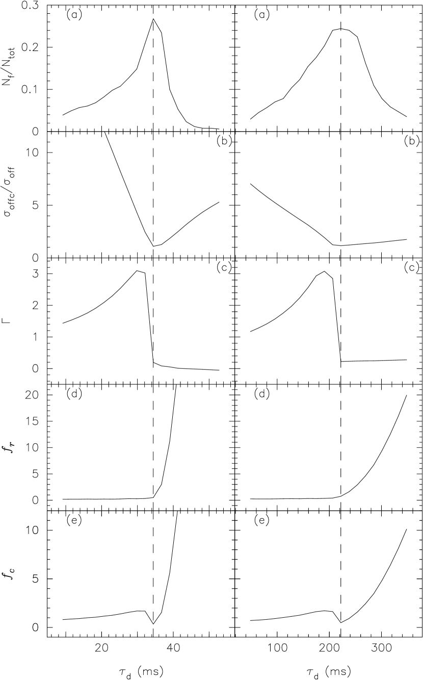
Figure 2: Plots of the various figures of merit used in the CLEAN method as a function of the model parameter, $\tau_{d}$. Left-hand side: simulated data from Figure 1. Right-hand side: real data from PSR J1852+0031 at 1475 MHz also in Figure 1. The vertical dashed lines show the true value of ${\tau_{d}}$ for the simulated case and the best value for the real data. (a) $N_{f}$, the number of data points within 3-$\sigma$ level of the noise, as described in the text; (b) $\mbox{${\sigma_{{\rm offc}}}$\,}/\mbox{${\sigma_{{\rm off}}}$\,}$, the ratio of RMS residual noise to the off-pulse RMS noise; (c) the skewness parameter, $\Gamma$; (d) the positivity parameter, $f_{r}$; and (e) the combined skewness + positivity parameter, $f_{c}=(\gamma+f_{r})/2$

As the deconvolution process removes smearing due to interstellar scattering, the resultant CLEANed pulse is narrower and the peak signal to noise (S/N) is higher, the increase being determined largely by the ratio of ${\tau_{d}}$ to pulse width. This is evident from examples of simulated and real data shown in Figs. 1 and 3–6; examination of Figure 1 suggests that the sum of CCs matches closely the area of the scattered pulse.

3 Further Examples

We illustrate the application of the above-described method using additional simulated and real data. In doing so, we show the sensitivity of the method for finding both the shape of the pulse broadening function and the appropriate ${\tau_{d}}$. We also demonstrate how the derived intrinsic pulse shapes vary with different PBFs.

3.1 Simulated Data

Pulse profiles are generated as single or multi-component Gaussians. Scattered profiles are then constructed for a given choice of PBF, and noise is added to the scattered profile to account for finite signal-to-noise ratios. The simulated scattered data are then input to our CLEAN algorithm to recover the intrinsic pulse shape as well as the best fit model PBF, and the results are compared with the original data and PBF used to generate the data. Figure 3 illustrates the case where the intrinsic pulse is a simple Gaussian and the ISM is described by a simple thin slab model. As evident from the figure, the intrinsic pulse obtained by application of the CLEAN algorithm is in very good agreement with the original data. A significant deviation from the best fit model PBF (a one-sided exponential with a characteristic timescale of 40 ms) leads to distortion of the resultant deconvolved pulse profile, leading to residual scattering (for PBFs narrower than the optimal case) or negative going features at trailing edge of the pulse (for PBFs wider than optimal case). This example thus demonstrates the ability of the technique to well characterize the PBF and recover the intrinsic pulse.

Fig 4 shows another example where the intrinsic pulse is modeled as a sum of Gaussians, to mimic a pulse profile that is composed of multiple components. As in the previous example, the ISM model assumed here is a thin slab of scattering material, which can be described by an exponential PBF with a characteristic time scale ${\tau_{d}}=60$ ms. The recovered pulse is in good agreement with the original data.

Figure 3: Example illustrating the CLEAN-based deconvolution for simulated data and trial PBFs having a range of pulse-broadening times. Top frame: the restored and true pulse shapes are shown as solid and dotted curves, respectively, along with the true PBF (a one-sided exponential with $\tau$ = 40 ms) used to generate the scattered pulse (dashed line). Lower panel: PBFs and resultant deconvolved pulse shapes for a range of models that have the correct PBF shape but a range of pulse-broadening times, ${\tau_{d}}=30,35,40,45$ and 50 ms, from top to bottom trace. PBFs that are narrower than the true PBF result in pulse shapes with residual scattering (${\tau_{d}}$=30 and 35 ms), while wider PBFs over-subtract the data, causing negative features near the trailing edge of the pulse (${\tau_{d}}$=45 and 50 ms).

Figure 4: Simulation example illustrating the CLEAN-based technique for recovering an intrinsic pulse shape consisting of three components. The CLEANed pulse (solid line) is overlayed on the original pulse (dotted line); the best fit PBF model (exponential with a time constant of 60 ms) is shown on the left (dashed curve).

3.2 Data from Observations

Having demonstrated the feasibility of the technique using simulated data, we now discuss its application to some real data. The data used in this paper are from recent observations at Arecibo, where a large sample of high-DM pulsars has been studied at multiple frequency bands (Bhat et al., 2002). The sample includes several new discoveries from the Parkes multibeam survey (Manchester et al., 2001) that are visible at Arecibo. Details of the observations and results will be presented in a forthcoming paper. Figure 5 shows the 1475 MHz profile of PSR J1852+0031 (B1849+00), whose DM$=680$ ${\rm pc\ cm^{-3}}$ implies a distance D$=8.4$ kpc using the model of Taylor & Cordes (1993). We attempted deconvolving these data with two widely different types of PBFs: (a) a sharp-edged PBF (eq. 3) that characterizes a thin slab model, (b) a rounded PBF (eq. 7) for a uniform distribution of scattering material. As the figure shows, the results are strikingly different; the final CLEAN pulse appears approximately triple for an exponential PBF (with a characteristic time ${\tau_{d}}$=225$\pm$14 ms), whereas it is a distinct double for the case of a uniform medium (${\tau_{d}}$=121$\pm$6 ms). At first glance, either of the models seem equally good. However, given that two-component profiles are more commonly observed at and near this radio frequency (which implies observations are more sensitive to a conal geometry than a core and cone case), we believe that a double profile is more likely. The double profile obtained with a rounded PBF is constituted from only 7 CCs, compared to 21 required to fit the data with an exponential PBF. As alluded to before, this economy in the number of CCs lends weight to the idea that the intrinsic profile is double. Very similar results are obtained for the same pulsar at 1175 MHz (Figure 6a), which implies that although the folded profile at 1475 MHz is an average from only $\sim$120 pulse periods, the result is not likely to be affected by inadequate profile stability.

More examples are shown in Figure 6, where the data span a wide range of signal to noise ratio and degree of scattering. The CLEAN method yields satisfactory and robust results even for cases where the scattering tail is not very prominent, as illustrated by the scattering tail of PSR J1902+0556, which extends only to a few percent of the pulse period. The 1175 MHz profile of PSR J1852+0031 illustrates the other extreme, where the scattering tail extends out to nearly half the pulse period. For the 430 MHz data on PSR J1901+0331, three different types of PBFs (eqs. 3, 7 and 7) were used for deconvolution. As evident from Figure 6c, the observations are better accounted for by a thin slab case with exponential PBF of ${\tau_{d}}$=60$\pm$3 ms or by a uniform medium with a PBF of characteristic time ${\tau_{d}}$=31$\pm$2 ms, rather than an intermediate case such as a thick slab (eq. 7). The residual asymmetry in the deconvolved pulse is most likely intrinsic to the pulsar beam, though it is possible that the true PBF for this line of sight differs from what we have considered. Detailed interpretations are deferred to a forthcoming paper where we will consider multifrequency data and additional forms for the PBF.

Figure 5: CLEANed pulse shapes for PSR J1852+0031 at 1475 MHz obtained by deconvolving with two different models for the PBF. The results are strikingly different. Upper panel: a one-sided exponential PBF, corresponding to a thin-screen model with a square-law structure function, yields ${\tau_{d}}$=225$\pm$14 ms and an approximately triple pulse with merged components. Lower panel: a more rounded PBF, corresponding to a uniform medium with a square-law structure function, yields ${\tau_{d}}$=121$\pm$6 ms and a distinct double pulse shape. The differences result from the fact that in the top panel, the sharp PBF requires broad structure in the deconvolved pulse in order to match the measured pulse. For the bottom panel, the PBF is more rounded and the deconvolved pulse can have sharper structure and still be consistent with the measured pulse.

Figure 6: The measured and CLEANed pulse profiles for four pulsars: (a) J1852+0031 at 1175 MHz, (b) J1853+0546 at 1475 MHz, (c) PSR J1901+0331 at 430 MHz; The measured pulse can be accounted for by either a thin slab model with a PBF of characteristic time, ${\tau_{d}}$=60$\pm$3 ms (dashed curves), or by a uniform medium with a PBF with ${\tau_{d}}$=31$\pm$2 ms (solid curves), and (d) PSR J1902+0556 at 430 MHz. The best fit ISM models (PBFs) are shown as dashed curves (panels $a$, $b$ and $d$), and the CLEANed pulses are shown as thick solid curves. The negative dip preceding the pulse in (a) is an artifact that appears for several choices of PBF and ${\tau_{d}}$.

Table 1: Pulse-broadening Times: Frequency Extrapolation vs CLEAN

				F-Extrapolation			CLEAN
PSR	DM	Distance	Frequency	${\tau_{d}}$	${\sigma_{\tau_{d}}}$		${\tau_{d}}$	${\sigma_{\tau_{d}}}$
	(${\rm pc\ cm^{-3}}$ )	(kpc)	(MHz)	(ms)	(ms)		(ms)	(ms)
J1852+0031	680	8.4	1175	367	75		487	73
J1852+0031	680	8.4	1475	190	30		225	14
J1853+0546	197.2	4.9	1175	12	2		13	2
J1853+0546	197.2	4.9	1475	6	1		6	1
J1855+0422	438.6	10.1	1175	25	15		24	4
J1901+0331	401.2	7.8	430	57	3		61	2
J1902+0556	179.7	3.9	430	15	3		14	1

3.3 Estimates of Pulse-broadening Time

The CLEAN-based approach we outlined in this paper provides a general tool that can be applied to a wide variety of measured pulse shapes and degrees of scattering. For pulse shapes that show significant scattering tails, application of the frequency extrapolation approach as outlined in §2.1 can be expected to yield satisfactory results. We have applied the CLEAN and frequency-extrapolation methods to strongly scattered pulses, such as those in Figure 6, and the results are tabulated in Table 1. The data span a wide range of DM, signal to noise ratio and degree of scattering. In the frequency extrapolation method, the uncertainty in ${\tau_{d}}$ is estimated as the model parameter range where ${\chi^{2}}$ is unity above the minimum. For the CLEAN method, a similar estimate can be defined based on the figure of merit parameter $f_{r}$, which is essentially an indicator of the average deviation of the residuals from the noise level (normalized to the noise variance). For instance, if a model results in a value for $f_{r}$ that is unity above that for the best fit PBF, then the pulse is over-subtracted by ${\sigma_{{\rm off}}}$ (on average). Note that the best fit model is characterized by a minimum in the combined figure of merit parameter $f_{c}$.

The CLEAN-based pulse-broadening measurements in Table 1 for PSRs J1852+0031 and J1853+0546 indicate scaling laws ${\tau_{d}}\propto\nu^{-x}$ with $x=3.45\pm 0.7$ and $x=3.4\pm 1.0$, respectively. These scalings may be compared with those expected from a Kolmogorov wavenumber spectrum with a negligibly small inner scale ($x=4.4$) or from a medium with a square-law structure function ($x=4$). The empirical intervals for $x$ include both cases, though the centroids of the intervals are certainly biased below the expected values. We defer a detailed analysis to a later paper, but we point out here that the inferred scaling index for a given pulsar will depend on the PBF used and that the PBF shape may also be a function of frequency. Ideally, the data and the CLEAN procedure will indicate the best PBF through investigation of the figures of merit discussed above. Both the PBF and the scaling index of ${\tau_{d}}$ are useful information for understanding the nature and distribution of scattering along the line of sight (Cordes & Lazio, 2001; Löhmer et al., 2001; Boldyrev & Gwinn, 2002). For multifrequency data like these, the CLEAN-based approach we have outlined here can be extended to do a global fit (by assuming the same form for the PBF, and ${\tau_{d}}$ scaling with the frequency as a power law but with an unknown index) to yield the pulse-broadening times and the index of the power law, along with the intrinisic pulse shapes. A detailed treatment of this approach is deferred to a forthcoming paper where we report on multifrequency pulse-broadening measurements for a larger sample of distant pulsars.

4 Conclusions

We have developed and applied an algorithm for deconvolving interstellar pulse broadening from radio pulses. The technique realizes the two-fold objective of recovering the intrinsic pulse shape and determining the pulse-broadening function that describes the scattering process. The method parallels the CLEAN algorithm used in synthesis imaging applications, but differs from CLEAN in that the best pulse broadening function is not known in advance. Additionally, we perform a true deconvolution, where the resolution of the deconvolved pulse is limited by the instrumental resolution rather than the pulse broadening function.

Application of the technique is demonstrated through use of simulated data as well as data from Arecibo observations. Unlike the conventional frequency extrapolation approach, the method makes no prior assumptions about the intrinsic pulse shape, and can therefore be applied to a wider variety of pulse shapes and degrees of scattering.

The derived intrinsic pulse shape depends on the form and parameters of the PBF used for deconvolving, and further considerations have to be employed to select the best fit model. We employ figures of merit that quantify positivity and asymmetry of the CLEANed pulse, and the best fit PBF is taken to be the one that yields minimal residual scattering and skewness of the intrinsic pulse. As in any other nonlinear method, the uniqueness of the deconvolved result is not always assured: however, further considerations (such as data at different observing frequencies) can help resolve any such degeneracy. Intrinsic pulse shapes obtained by application of this method are likely to be closer to reality, and hence should prove to be useful for the study of pulsar emission properties. A paper is in preparation which applies our method to a large body of multi-frequency pulsar observations.

References

- Armstrong, Rickett & Spangler (1995) Armstrong, J. W., Rickett, B. J., & Spangler, S. R. 1995, ApJ, 443, 209.
- Bhat et al. (2002) Bhat, N. D. R., Camilo, F., Cordes, J. M., Nice, D. J., Lorimer, D. R., Chatterjee, S. 2002, JA&A, Accepted.
- Boldyrev & Gwinn (2002) Boldyrev, S., & Gwinn, C. R. 2002, ApJ, Submitted.
- Cordes & Lazio (1991) Cordes, J. M. & Lazio, T. J. 1991, ApJ, 376, 123.
- Cordes & Lazio (2001) Cordes, J. M. & Lazio, T. J. W. 2001, ApJ, 549, 997.
- Cordes & Rickett (1998) Cordes, J. M. & Rickett, B. J. 1998, ApJ, 507, 846.
- Cornwell, Braun & Briggs (1999) Cornwell, T., Braun, R., & Briggs, D. S. 1999, ASP Conf. Ser. 180: Synthesis Imaging in Radio Astronomy II, 151.
- Hankins & Rickett (1986) Hankins, T. H. & Rickett, B. J. 1986, ApJ, 311, 684.
- Högbom (1974) Högbom, J. A. 1974, A&AS, 15, 417.
- Kuz’min & Izvekova (1993) Kuz’min, A. D. & Izvekova, V. A. 1993, MNRAS, 260, 724
- Lambert & Rickett (1999) Lambert, H. C. & Rickett, B. J. 1999, ApJ, 517, 299.
- Löhmer et al. (2001) Löhmer, O., Kramer, M., Mitra, D., Lorimer, D. R., & Lyne, A. G. 2001, ApJ, 562, L157.
- Manchester et al. (2001) Manchester, R. N. et al. 2001, MNRAS, 328, 17.
- Rickett (1990) Rickett, B. J. 1990, ARA&A, 28, 561.
- Roberts, Lehar & Dreher (1987) Roberts, D. H., Lehar, J., & Dreher, J. W. 1987, AJ, 93, 968
- Schwarz (1978) Schwarz, U. J. 1978, A&A, 65, 345.
- Taylor & Cordes (1993) Taylor, J. H. & Cordes, J. M. 1993, ApJ, 411, 674.
- Weisberg et al. (1990) Weisberg, J. M., Pildis, R. A., Cordes, J. M., Spangler, S. R., & Clifton, T. R. 1990, BAAS, 22, 1244.
- Williamson (1972) Williamson, I. P. 1972, MNRAS, 157, 55.
- Williamson (1973) Williamson, I. P. 1973, MNRAS, 163, 345.