RELATIVISTIC JETS IN COLLAPSARS

Abstract

We examine the propagation of two-dimensional relativistic jets through the stellar progenitor in the collapsar model for gamma-ray bursts (GRBs). Each jet is parameterized by a radius where it is introduced, and by its initial Lorentz factor, opening angle, power, and internal energy. In agreement with previous studies, we find that relativistic jets are collimated by their passage through the stellar mantle. Starting with an initial half-angle of up to 20 degrees, they emerge with half-angles that, though variable with time, are around 5 degrees. Interaction of these jets with the star and their own cocoons also causes mixing that sporadically decelerates the flow. We speculate that this mixing instability is chiefly responsible for the variable Lorentz factor needed in the internal shock model and for the complex light curves seen in many gamma-ray bursts. In all cases studied, the jet is shocked deep inside the star following a brief period of adiabatic expansion. This shock converts most of the jet’s kinetic energy into internal energy so that even initially “cold” jets become hot after going a short distance. The jet that finally emerges from the star thus has a moderate Lorentz factor, modulated by mixing, and a very large internal energy. In a second series of calculations, we follow the escape of that sort of jet. Conversion of the remaining internal energy gives terminal Lorentz factors along the axis of approximately 150 for the initial conditions chosen. Because of the large ratio of internal to kinetic energy in both the jet ($\geq 80\%$) and its cocoon, the opening angle of the final jet is significantly greater than at breakout. A small amount of material emerges at large angles, but with a Lorentz factor still sufficiently large to make a weak GRB. This leads us to propose a “unified model” in which a variety of high energy transients, ranging from x-ray flashes to “classic” GRBs, may be seen depending upon the angle at which a standard collapsar is observed. We also speculate that the breakout of a relativistic jet and its collision with the stellar wind will produce a brief transient with properties similar to the class of “short-hard” GRBs. Implications of our calculations for GRB light curves, the luminosity-variability relation, and the GRB-supernova association are also discussed.

1 INTRODUCTION

Growing evidence connects GRBs to the death of massive stars. Analysis by Frail et al. (2001) and others of the radio afterglows of “long-soft” GRBs suggests that, despite great diversity in apparent brightnesses, these events have a total kinetic energy in relativistic matter tightly clustered around $3\times 10^{51}\,{\mathrm{erg}}$ (Frail et al., 2001) - a supernova-like energy. “Bumps” resembling the light curves of Type I supernovae have also been seen in the optical afterglows of at least four GRBs (GRB 980326, Bloom et al. 1999; GRB 970228, Reichart 1999, Galama et al. 2000; GRB 011121, Bloom et al. 2002, Garnavich et al. 2002; and GRB 020405, Price et al. 2002) and GRB 980425 has been associated with an optical supernova, SN 1998bw (e.g., Galama et al. 1998; Iwamoto et al. 1998; Woosley, Eastman, & Schmidt 1999). The observational evidence that (long-soft) GRBs are associated with regions of star formation has become overwhelming (Bloom, Kulkarni, & Djorgovski, 2002). Given the evidence for beaming and relativistic motion, it is probable that at least one major subclass of GRBs is a consequence of massive stars that, in their explosive deaths, produce relativistic jets.

Here we examine the passage of relativistic jets through a collapsing massive star and their breakout. We begin with a rotating star that has already experienced 10 seconds of collapse. Ten seconds is the nominal time for a disk to form around a black hole and the polar region to become sufficiently evacuated for a polar jet to propagate (MacFadyen & Woosley, 1999). The initial progenitor is a helium core of $15\,M_{\sun}$ evolved by Heger & Woosley (2002) to iron core collapse with approximations to all (non-magnetic) forms of angular momentum transport included. The missing 10 seconds is followed using a non-relativistic two-dimensional code as in MacFadyen & Woosley (1999). We pick up the calculation when the jet, which presumably began in a region $\sim 30\,{\mathrm{km}}$ in size, has already reached a radius of $2000\,{\mathrm{km}}$ and do not consider what has gone on inside. For present purposes, details of whether the jet was made by black hole angular momentum, MHD processes in the disk, or neutrinos do not concern us. The jet is initiated in a parametric way based upon its power, opening angle, Lorentz factor, and internal energy. Its propagation to the stellar surface at $800,000\,{\mathrm{km}}$, and its interaction with the stellar mantle is then followed (§ 3.1). Additional calculations (§ 3.3) also examine what happens to the jet immediately after it escapes the star and converts its residual internal energy into additional relativistic motion.

We find, in agreement with Aloy et al. (2000), that the passage of the jet through the star leads to its additional collimation. We also find that instabilities along the beam’s surface lead to mixing with the nearly stationary stellar material and cocoon. The mixing produces variations in the mass loading, and therefore the Lorentz factor of the jet. The opening angle of the jet also varies with time, gradually, if irregularly, growing as the star is blown aside. These results, discussed in § 4, have important implications for the observed light curves and energies of GRBs and imply that what is seen may vary greatly with viewing angle. In particular, we predict the existence of a large number of low energy GRBs with mild Lorentz factors (§ 4.3) that may be related to GRB 980425/SN 1998bw and to the recently discovered “hard x-ray flashes” (Heise et al., 2001).

Finally, we consider the breakout of the jet. As the shock breaks out a small amount of material being pushed ahead by the jet head is accelerated to relativistic speeds. Interaction of this material with the stellar wind of the progenitor will produce a transient of some sort (Woosley, Eastman, & Schmidt, 1999; Tan, Matzner & McKee, 2001). We speculate that this is the origin of a hard precursor to GRBs that, at least in some cases, might be characterized as a “short-hard GRB” in isolation(§ 4.4).

2 COMPUTATIONAL PROCEDURE AND ASSUMPTIONS

2.1 The Relativistic Code Employed

In order to study relativistic jets in collapsars, we developed a special relativistic, multiple-dimensional hydrodynamics code similar to the GENESIS code (Aloy et al., 1999). Our program employs an explicit Eulerian Godunov-type method with numerical flux calculated using an approximate Riemann solver: Marquina’s flux formula. The PPM algorithm is used to reconstruct the variables so that high-order spatial accuracy is achieved. Second- or third-order Runga Kutta methods are employed for the time integration. This method has previously been used successfully to study relativistic jets in collapsars and many other ultra-relativistic flows (Aloy et al., 1999). The code has been extensively tested and the results are comparable with those found in the literature (Martí & Müller, 1999, and references therein). To model collapsars more accurately, the code was revised to include a realistic equation of state (Blinnikov, Dunina-Barkovskaya, & Nadyozhin, 1996), that, in particular, allows a Fermi gas of electrons and positrons with arbitrary relativity and degeneracy. Radiation and an ideal gas of nuclei are also included. The code was also modified to include the advection of nuclear species. Nuclear burning, which is not important in the present problem, is not considered. Because we are interested in phenomena far from the central black hole, gravity is treated in the Newtonian approximation. We do not include the self gravitational force of the mass on our grid, but only a radial force from the mass inside our inner boundary condition.

2.2 The Stellar Model

Our initial model is derived from a 15 $M_{\sun}$ helium star of 0.1 solar metallicity with an initial surface rotation rate of 10% Keplerian on the helium burning main sequence. This Wolf-Rayet star might be the result of a star with initially 40 $M_{\sun}$ on the main sequence. The rotating helium star is evolved to iron core collapse (defined as when any part of the star is collapsing at $10^{8}\,{\mathrm{cm}}\,{\mathrm{s}}^{-1}$) including angular momentum transport, but neglecting mass loss and magnetic fields (Heger, Langer, & Woosley 2001; Heger & Woosley 2002). It is presumed that this helium star has lost its hydrogen envelope either to a companion star or by stellar winds. The collapsing, but still initially spherical star is mapped into a two-dimensional non-relativistic code (MacFadyen & Woosley, 1999) and the inner 2 $M_{\sun}$ of iron core, which is assumed to collapse to a black hole, replaced by an absorbing inner boundary condition at $10^{7}\,{\mathrm{cm}}$. Poisson’s equation is then solved using a post-Newtonian gravitational potential. Neutrino cooling by thermal processes and pair capture are included, as well as the photodisintegration of nuclei into nucleons in the inner part of the disk, once one has formed. The calculation is run until a low density channel ($\rho\lesssim 10^{6}\,\mathrm{g}\,{\mathrm{cm}}^{-3}$) has cleared along the rotational axis. This takes approximately $10\,{\mathrm{s}}$ after the initial core collapse. The collapsing rotating star is then mapped into our two-dimensional special relativistic code(§ 2.1), the inner boundary moved out to $2\times 10^{8}\,{\mathrm{cm}}$, and a $5.0\,M_{\sun}$ point mass placed at its center.

During this $10\,{\mathrm{s}}$, rotation and infall appreciably modify the core structure, but only inside of $5000\,{\mathrm{km}}$. Outside $10,000\,{\mathrm{km}}$, one might just as well use a non-rotating presupernova model. The present study with an inner boundary at $2000\,{\mathrm{km}}$ is thus moderately sensitive to the post-collapse evolution of the rotating progenitor. For example, the density in the equatorial plane at $2000\,{\mathrm{km}}$ and $10\,{\mathrm{s}}$ is ten times greater than that at the same radius along the axis. However, this non-spherical density structure does not critically influence jet propagation. Our two-dimensional starting model is available to others and might be the basis for comparison calculations that are more sensitive to the structure of the inner star.

2.3 Initial Conditions

A two-dimensional spherical grid ($r,\theta$) is employed consisting of 480 logarithmically spaced radial zones, 120 uniform angular zones in the polar region ($0\arcdeg\leq\theta\leq 30\arcdeg$) and 80 logarithmically spaced angular zones in the range $30\arcdeg\leq\theta\leq 90\arcdeg$. The initial model is remapped onto this grid with an inner boundary at $2\times 10^{8}\,{\mathrm{cm}}$, and an outer boundary at $9\times 10^{10}\,{\mathrm{cm}}$.

As the initial condition for the calculation, a highly relativistic jet is assumed to have formed interior to the inner boundary of the computational grid. The jet is implemented in the calculation as an inner boundary condition. An axisymmetric outflow is injected in a purely radial direction through the inner boundary at $2\times 10^{8}\,{\mathrm{cm}}$ within a half-angle $\theta\leq\theta_{0}$, where $\theta_{0}$ is a free parameter. The processes producing the jet are uncertain, but are presumed to have endowed it with a large energy per baryon. At the origin this may have been in the form of a large internal energy (as in the neutrino-version of the collapsar model or a jet energized by magnetic reconnection) or the jet may have been born with low entropy and highly directed motion (as in some versions of MHD accelerated jets). As we shall see, processes deep inside the star tend to erase the distinction.

The jet is specified by its power, $\dot{E}$, initial opening half-angle, $\theta_{0}$, initial Lorentz factor, $\Gamma_{0}$, and the ratio of its kinetic energy to its total energy, $f_{0}$. Of these four parameters, the power is the easiest to address. First, observationally, we know that the total energy in relativistic ejecta is of order a few times $10^{51}\,{\mathrm{erg}}$ for the entire event (e.g., Frail et al. 2001). The energy in subrelativistic ejecta, i.e., the supernova, is probably comparable or greater (Woosley et al. 1999; Iwamoto et al. 1998). A total energy of order $10^{52}\,{\mathrm{erg}}$ is thus reasonable. From another perspective, roughly one to several solar masses of material will accrete into the black hole during the principal phase of the GRB. If a few tenths of a percent of the rest mass energy is used to power jet-like outflows, one again obtains $\sim 10^{52}\,{\mathrm{erg}}$. In the lab frame, the duration of a (long-soft) GRB is $\sim 10\,{\mathrm{s}}$, so a jet power of $10^{51}\,{\mathrm{erg}}\,{\mathrm{s}}^{-1}$ is reasonable and probably accurate to an order of magnitude. We employed this energy for each jet so that the total is $2\times 10^{51}\,{\mathrm{erg}}\,{\mathrm{s}}^{-1}$ (or $2\times 10^{52}\,{\mathrm{erg}}$ in $10\,{\mathrm{s}}$). In light of recent developments that have tended to downgrade the total energy of a GRB to a few times $10^{51}\,{\mathrm{erg}}$ (Frail et al., 2001) and even suggest that the kinetic energy after the GRB is over is only a few times $10^{50}\,{\mathrm{erg}}$ (Panaitescu & Kumar, 2001), this may be too large. So we also ran one set of calculations with an energy 30% as great. This is still large compared with the estimate by Panaitescu & Kumar (2001).

The ratio of kinetic energy to total energy, $f_{0}$, depends on how the jet was born and its history before it entered the computational grid and is more difficult to estimate. We assume, at $2000\,{\mathrm{km}}$, that our jet has comparable internal and kinetic energies in the laboratory frame. Specifically, we adopt an initial Lorentz factor, $\Gamma$, of 50 for Models JA and JB, and $f_{0}=1/3$. These values are reasonable for a jet which began at say $30\,{\mathrm{km}}$ consisting initially of a small amount of matter at rest with about $\sim 150$ times its rest mass in internal energy. That is, in the notation of Mészáros, Laguna, & Rees (1993), $\eta=150$. For a jet of constant opening angle, $\theta_{0}$, the Lorentz factor of an adiabatically expanding jet scales as $\sim r$. If $\theta_{0}$ decreases with $r$ inside of $2000\,{\mathrm{km}}$ as is likely, $\Gamma$ grows more gradually. For the parameters chosen in Table 1, the terminal Lorentz factors of the jets if they expanded freely to infinity would be 150 for Models JA and JB. We also explored, for comparison, Model JC which had a lower initial Lorentz factor and a smaller total power, but a larger fraction of internal energy (Table 1). Fortunately, as we shall see, the initial partition of energy is not an important parameter of the model - so long as the total energy per baryon is large.

3 RESULTS

Because of the difficulty of carrying too large a range of radii on the computational grid, each calculation was carried out in two stages: 1) propagation inside the star, and 2) propagation in the stellar wind after breakout. The calculations, although two-dimensional, did not include the dynamical effects of rotation in the jet.

3.1 Jet Propagation Inside the Star

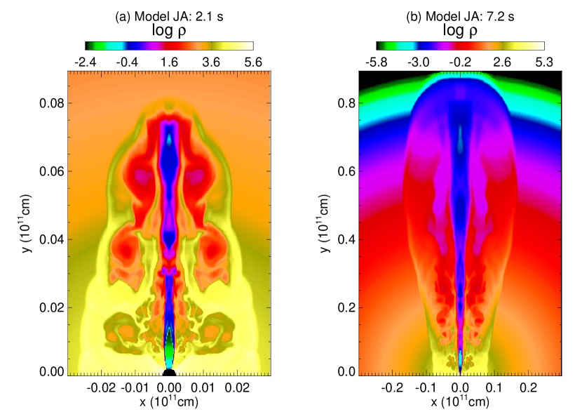
Figure 1: Density structure in the local rest frame for Model JA at (a) $t=2.1\,{\mathrm{s}}$ (left) and (b) $7.2\,{\mathrm{s}}$ (right). In (a), only the central region of the star is shown. The radius of the star is $8\times 10^{10}\,{\mathrm{cm}}$. Note the morphological differences among Models JA (Fig. 1), JB (Fig. 2) and JC (Fig. 3).

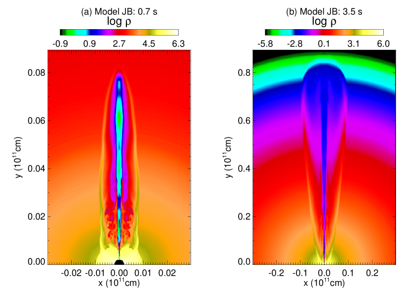
Figure 2: Density structure in the local rest frame for Model JB at (a) $t=0.7\,{\mathrm{s}}$ (left) and (b) $3.5\,{\mathrm{s}}$ (right). In (a), only the central region of the star is shown. Note the much higher degree of collimation than in Model JA.

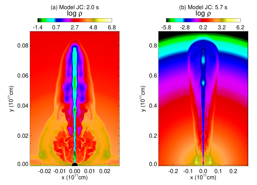
Figure 3: Density structure in the local rest frame for Model JC at (a) $t=2.0\,{\mathrm{s}}$ (left) and (b) $5.7\,{\mathrm{s}}$ (right). In (a), only the central region of the star is shown. Note the shape of bow shock in (a) and contrast to Fig. 1.

In all models the jet initially propagates along the polar axis. After a short time, it consists of a supersonic beam; a cocoon consisting of shocked jet material and shocked medium gas; a terminal bow shock; a working surface; and backflows (Blandford & Rees, 1974). Some snapshots of the jet for the three models JA, JB and JC, as defined in Table 1, are shown in Figures 1, 2 and 3. In all models, the jet is narrowly collimated and its beam is very thin, but other aspects of jet morphology vary from model to model. In Model JA, because of its large initial opening angle, most of the jet material passes, early on, through a strong shock, which deflects the flow toward the axis. In Model JB, which has a smaller initial opening angle and denser beam, the momentum flux is larger than for Model JA. The jet head thus advances faster and the beam is almost naked with a very thin cocoon. In Model JC, the thickness of the cocoon and beam and the velocity of the jet head are intermediate between JA and JB. At early times, the bow shock has a narrow head and wide tail (Fig. 3a), reflecting the jet’s acceleration. At late times however, especially as the jet nears the surface of the star, the morphologies of all three models are very similar (Fig. 1b, 2b and 3b). This suggests that the initial conditions tend to be forgotten as the jets propagate and interact with the star. It also implies that the properties of the subsequent GRB may not be sensitive to details of the operation of the central engine.

Because of the ram pressure of infalling stellar material at $2000\,{\mathrm{km}}$, a jet cannot start immediately. It must build up some pressure on the grid. In Model JA, 0.6 second elapses (in addition to the $10\,{\mathrm{s}}$ since core collapse) before the jet starts to propagate appreciably along the polar axis. The corresponding delays are 0.1 second and 0.3 second for Models JB and JC, respectively. Once they get going, the times for the jets to traverse the star (outside of $2000\,{\mathrm{km}}$) and break out also vary: 6.9, 3.3 and 5.5 seconds for Models JA, JB and JC, respectively (Table 2). This is reasonable since the jet in Model JB has a smaller cross section area and a larger momentum flux than in Models JA and JC.

Along the polar axis, the beam in each model is divided into two regions: an unshocked region and a shocked region (Fig. 4, 5 and 6). Because of its low density, low pressure, and relativistic velocity, the jet initially creates a low-density, low-pressure funnel along the axis. Within this funnel, the jet is steady and expands adiabatically without internal shocks. The high Lorentz factor helps to suppress the Kelvin-Helmholtz instability.

Farther out though, the jet head makes its way through the star at a sub-relativistic speed of roughly $c/2$ (this speed increases as the jet head moves outward in radius). Cocoon material flows back from the working surface. Relativistic material moving along the axis runs into comparatively stationary stellar matter at the jet head and pressure grows in this backed up material until it becomes comparable to that in the cocoon, which is in turn somewhat greater than the surrounding stellar medium. Then lateral expansion can occur. The need for deceleration propagates inwards in jet mass - though its location still moves outward in radius - as a reverse shock. At this inner shock the adiabatically expanding jet has a ram pressure, $\sim\rho h\Gamma^{2}c^{2}$, which approximately balances the pressure in the shocked jet, here $h$, the specific enthalpy, is $(e+p)/(\rho c^{2})$, where, $e$, the total energy density, includes rest mass density.

To summarize, as seen by a piece of jet starting at the origin: 1) internal energy is converted to expansion until the reverse shock is encountered; 2) kinetic energy is then converted mostly back into internal energy at the reverse shock, though the motion remains moderately relativistic ($\Gamma\sim 5-10$); and 3) the hot jet is further decelerated to subrelativistic speeds at the jet head. In what follows we shall refer to jet material in stage 1 as the “unshocked jet” and stage 2 as the “shocked jet”.

The interaction of the shocked jet with the star is especially interesting since Kelvin-Helmholtz instabilities and oblique shocks inside the cocoon can imprint time structure on its Lorentz factor (see also Martí et al. 1997 and references therein). The consequences differ in the three models. Because of its larger initial opening angle, the jet in Model JA experiences a stronger deceleration at the reverse shock, so the average Lorentz factor of the shocked jet in Model JA is lower than for Models JB and JC. In Model JA, the head of the unshocked jet (i.e., the location of the reverse shock) moves outward with a gradual acceleration. In Model JC the speed is almost constant, but, in Model JB, the location of this shock even moves backwards sometimes.

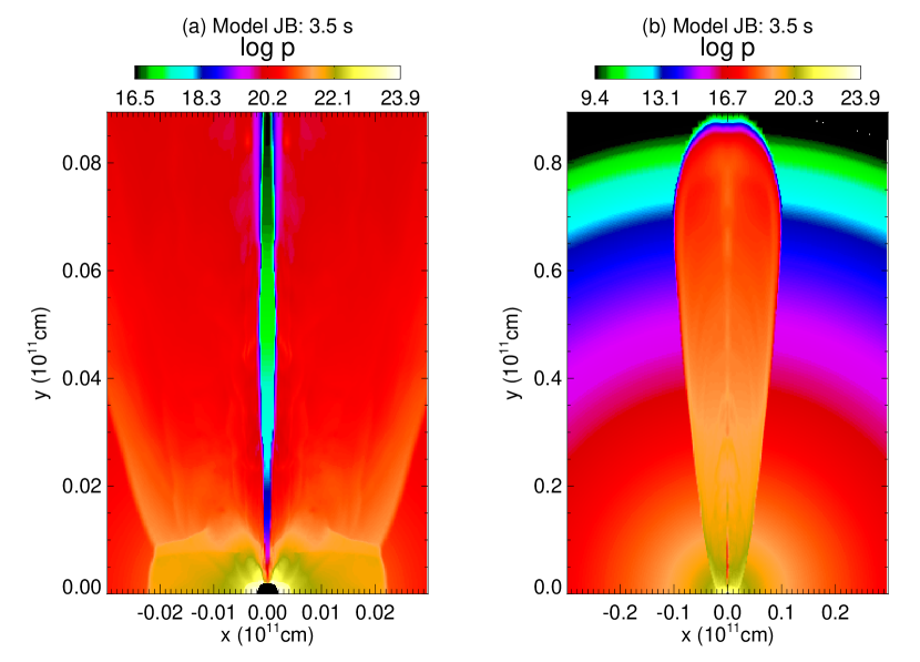
Figure 7: Pressure in Model JB at $t=3.5\,{\mathrm{s}}$. In (a) (left) only the central region of the star is shown. In (b) (right), the whole star is shown. The radius of the star is $8\times 10^{10}\,{\mathrm{cm}}$. In the central region, the pressure in the jet beam is much lower than that in the medium. The overall structure of pressure is smooth.

A possible explanation is that the unshocked jet in Model JB is unstable to pinching modes of the Kelvin-Helmholtz instability. It has been shown numerically (Martí et al., 1997) and analytically (Ferrari, Trussoni, & Zaninetti, 1978) that ultra-relativistic jet beams tend to be unaffected by the Kelvin-Helmholtz instability. However, small scale perturbations might still be able to grow if the jet beam is very thin (Ferrari, Trussoni, & Zaninetti, 1978). It is also important that these other works assumed equal pressures in the beam and external medium. Here the jet is under-pressurized compared to the medium (Fig. 7). When the mixing between jet beam and nearly stationary stellar material occurs, the beam will be decelerated. This behavior imprints time structure on the Lorentz factor which consequently turns out to be more variable Model JB than Models JA and JC. Some implications of this will be discussed in § 4.

As the jets pass through the star, they are narrowly collimated by the external pressure (Fig. 8). Near the origin, opening angles of jet beams are close to their initial values, $20\arcdeg$, $5\arcdeg$, and $10\arcdeg$ for Models JA, JB, and JC, respectively. In the unshocked region, the jet beam forms a low-pressure funnel that is quickly focused by the high pressure of the external stellar matter. In Model JA at $t=12.0\,{\mathrm{s}}$ for example, the half opening angle of the jet beam has already decreased to $\sim 10\arcdeg$ at $r=8.2\times 10^{9}\,{\mathrm{cm}}$, only $1/10$ of radius of the star (Fig. 8).

In the shocked jet the pressure is larger than in the external medium. The jet beam is surrounded by an over-pressurized cocoon which is in turn in balance with the star. There are no longer dramatic changes in $\theta_{0}$ in this shocked region. (Fig. 8). At the surface of the star, the half opening angles of the jet beams have decreased to very similar values, $\sim 4\arcdeg$, $\sim 2\arcdeg$, and $\sim 3\arcdeg$, for Models JA at $t=12.0\,{\mathrm{s}}$, JB at $t=8.0\,{\mathrm{s}}$, and JC at $t=10.0\,{\mathrm{s}}$, respectively. Still there are interesting differences among the models. Model JA which started with the largest initial angle still has the greatest angle at breakout. On the other hand, the energy flux per solid angle in Model JB is higher. Thus along the jet it would appear brighter. The distribution of energy with angle is also interesting. In Model JA, the jet is “hollow”, but in Models JB and JC, peak flux occurs on axis. Fig. 9 also shows that the opening angle in Model JA is increasing as the jet blows off the star. All of these effects, different intensities per solid angle, more rapidly variable Lorentz factor in Model JA, changing opening angle with time, etc. will have important consequences for the GRB light curves and its afterglows.

3.2 The Emergence of the Jet

Eventually, the jet accelerates and breaks free of the star. In Model JA, the average velocity of the head of the jet just prior to breakout is $1.2\times 10^{10}\,{\mathrm{cm}}\,{\mathrm{s}}^{-1}$. For Models JB and JC the speeds are $2.5\times 10^{10}\,{\mathrm{cm}}\,{\mathrm{s}}^{-1}$ and $1.5\times 10^{10}\,{\mathrm{cm}}\,{\mathrm{s}}^{-1}$ respectively. Of course the speeds behind the jet head and in the beam are higher, $\Gamma\sim$ 10, 50, and 20 for Models JA, JB and JC, respectively (Fig. 10). These would be regarded by most as too low to produce healthy GRBs (e.g., Lithwick & Sari 2001). However, these jets still have a large ratio of internal energy to total energy: $\sim$ 80-95%, $\sim$ 50-75%, and $\sim$ 80-90% for Models JA, JB and JC. That is the jets themselves are still fireballs with $\eta\sim$ 3 to 10. After all internal energy is converted to kinetic energy, the terminal Lorentz factor will still be $\sim$ 100-200. This implies that despite being shocked deep inside the star and experiencing Kelvin-Helmholtz instabilities, the matter that emerges has almost the same energy per baryon that it started out with at $2000\,{\mathrm{km}}$. The baryonic entrainment has been small. Of course this result needs to be tested in a three dimensional calculation, but it is encouraging.

After breakout, a channel is open through which the jet can propagate without losing much energy (though it is still shocked and modulated while passing through the star). The total power carried by matter with Lorentz factor greater than 10 is $\sim 0.9\times 10^{51}\,{\mathrm{erg}}\,{\mathrm{s}}^{-1}$, $\sim 1\times 10^{51}\,{\mathrm{erg}}\,{\mathrm{s}}^{-1}$ and $\sim 3.0\times 10^{50}\,{\mathrm{erg}}\,{\mathrm{s}}^{-1}$ just after breakout for Models JA, JB and JC, respectively (Fig. 11). Those are very close to the initial values at the inner boundary (Tab. 1).

By the time of breakout, the total energy injected as twin jets was 13.8, 6.6, and $3.3\times 10^{51}\,{\mathrm{erg}}$ in Models JA, JB, and JC respectively. The energy on the grid in various forms is given at that time in Table 2. In particular we can estimate the available energy to produce a supernova, $E_{\mathrm{sn}}$, from the total energy in matter moving at less than 10% the speed of light ($\Gamma<1.005$) by considering corrections due to initial energy and energy lost at the computational inner boundary. The jet propagates very efficiently through the star after breakout (Fig. 11) so that there is very little further “wasted” energy available for powering a supernova in any of the models. However, one should keep in mind a) that some non-relativistic energy may still be available to power the supernova as the jet starts to die off, and b) the wind off the accretion disk may also contribute significant energy to the explosion (MacFadyen & Woosley 1999). The supernova energies in Table 2 are thus lower bounds for the (admittedly high) jet energies assumed.

We followed Models JA, JB, and JC for a total of $21.8\,{\mathrm{s}}$, $10.0\,{\mathrm{s}}$, and $15.0\,{\mathrm{s}}$ respectively (Table 3) and their total energies were these times multiplied by the assumed injection rates (Table 1). Before breakout some energy is “wasted” because the head of the jet moves much slower than the jet itself. The amount of “wasted” energy is given by, $E_{\mathrm{c}}=2\dot{E}(t_{\mathrm{b}}-R_{\mathrm{s}}/c)$, where $\dot{E}$ is the power at the base for each jet, $t_{\mathrm{b}}$ is the time for the jet to break out of the star, and $R_{\mathrm{s}}$ is the stellar radius. Using this expression, we estimate the sums of the energies in the supernova and jet cocoon (Table 3). Most of this energy is in non-relativistic hot material near the jet which can power the supernova; the remainder is in the cocoon which emerges from the star (Ramirez-Ruiz, Celotti, & Rees, 2002).

The history of Lorentz factor at the edge of our computational grid on the polar axis is shown in Fig. 10. This figure also shows the estimated terminal Lorentz factor if all internal energy is converted into kinetic energy and the process is adiabatic. The fluctuations of the Lorentz factor are not so large as to make efficient internal shocks, but our grid is relatively coarse and numerical viscosity may wash out most fluctuations, especially those due to small scale instabilities. Because of the large range of radii covered, our two-dimensional spherical grid consists of logarithmically spaced radial zones, and both uniform and logarithmically angular zones. This gives good resolution at the center, but unfortunately the resolution near the edge of the star is too low to study the details of time structure. The Lorentz factor along the polar axis at $4.0\,{\mathrm{s}}$ in Model B contains many significant fluctuations (Fig. 5), but these are smoothed quickly by numerical viscosity. In the near future we plan further calculations using cylindrical geometry and finer resolution to study the mixing better.

When the jet breaks out, it is the hot shocked beam that emerges first. If the engine lasts long enough, the unshocked beam may eventually emerge, e.g. at $\sim 20$ s in Model JA (Fig. 4; remember that $10\,{\mathrm{s}}$ must be added to all our times to get the time when the core actually collapsed). In Model JB, the mixing instability caused by the interaction among the jet beam, cocoon and star slows the jet more. About 6.7 seconds after breakout, the head of the unshocked jet is still only at at $2.5\times 10^{9}\,{\mathrm{cm}}$ while in Model JC it is at $7.9\times 10^{9}\,{\mathrm{cm}}$. Because more than half of the total energy in the shocked jet material is in form of internal energy, it is inevitable that the jet will experience acceleration and, possibly, sideways expansion. What is the final opening angle of the jet? What is the final Lorentz factor of the jet as the internal energy is converted into kinetic energy? In order to power a GRB, the jet has to have a Lorentz factor of more than 100. Can the shocked mildly relativistic jet ($\Gamma\sim 10-50$) acquire high enough Lorentz factor ($\Gamma>100$) after breakout?

3.3 Jet Propagation in the Near Stellar Environment

After it breaks out of the star, the relativistic jet, which has a high internal energy loading, accelerates and spreads. It also encounters the stellar wind surrounding the star. In a second series of calculations we explored, in a preliminary way, this expansion. The jet is once more specified by its energy deposition rate, $\dot{E}$, initial opening angle, $\theta_{0}$, initial Lorentz factor, $\Gamma_{0}$, and the ratio of kinetic energy to total energy, $f_{0}$. Two models were considered (Table 4): (W1) $\dot{E}=8\times 10^{50}\,{\mathrm{erg}}\,{\mathrm{s}}^{-1}$, $\theta_{0}=3\arcdeg$, $\Gamma_{0}=10$, $f_{0}=0.06$; (W2) $\dot{E}=8\times 10^{50}\,{\mathrm{erg}}\,{\mathrm{s}}^{-1}$, $\theta_{0}=3\arcdeg$, $\Gamma_{0}=50$, $f_{0}=0.33$. These conditions are representative of the actual conditions in the emerging jets for Models JA, JB, and JC.

Because, for this set of calculations, we are not so interested in what happens close to the stellar surface, a two-dimensional cylindrical grid ($r,z$) is employed consisting of 2400 zones in $z$-direction from $10^{11}\,{\mathrm{cm}}$ to $1.3\times 10^{12}\,{\mathrm{cm}}$ and 720 zones in $r$-direction from $0$ to $3.6\times 10^{11}\,{\mathrm{cm}}$. Due to the relativistic velocities and large radius we can ignore gravity. A gamma-law equation of state with $\gamma=4/3$ also suffices. The background density, which might come from stellar mass loss, has been assumed to decline as $\rho\sim R^{-2}$, and the density at $R=10^{11}\,{\mathrm{cm}}$ is set to $3.7\times 10^{-11}\,\mathrm{g}\,{\mathrm{cm}}^{-3}$, which roughly corresponds to a mass loss of $\sim 10^{-5}\,M_{\sun}\,{\mathrm{yr}}^{-1}$ with a velocity of $\sim 1000\,\mathrm{km}\,\mathrm{s}^{-1}$. Actually, the details of environment are unimportant here because we have not yet followed the jet to such large radii that the interaction with the wind becomes important. The jet is injected at $z=10^{11}\,{\mathrm{cm}}$ with an opening angle of $3\arcdeg$ with momentum that is purely radial. Though potentially quite important, to keep things simple, we do not include a cocoon in these calculations. Also for simplicity, the jet is given uniform initial properties within its opening angle.

In our simulations, the jets are injected with the constant properties specified above for the first 10 seconds. Eventually though, we expect the central engine to decline in power and produce a less energetic jet. To mimic this decline, the jet energy and Lorentz factor were both turned down during the interval 10 to $20\,{\mathrm{s}}$ while the pressure and density of the jet were kept constant. The energy deposition rate decreased linearly from $8\times 10^{50}\,{\mathrm{erg}}\,{\mathrm{s}}^{-1}$ at $t=10\,{\mathrm{s}}$ to 0 at $t=20\,{\mathrm{s}}$ (Fig. 12). After 20 seconds, we used an outflow (zero gradient) boundary condition for the lower $z$ boundary. The total energy for each jet is thus $1.2\times 10^{52}\,{\mathrm{erg}}$ for both Models W1 and W2.

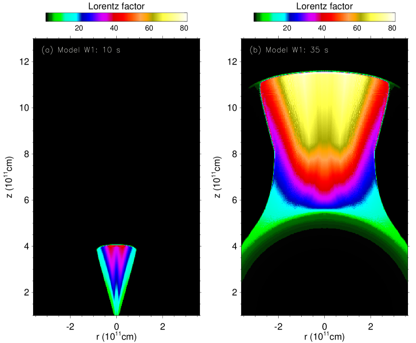
Figure 13: Lorentz factor for Model W1 at (a) $t=10\,{\mathrm{s}}$ (left) and (b) $t=35\,{\mathrm{s}}$ (right) after the jets start to propagate in the stellar wind. The initial opening angle is $3\arcdeg$. At $t=35\,{\mathrm{s}}$, the opening angle is $\sim 15\arcdeg$, which is much bigger than that of Model W2 at the same time. Because the power and Lorentz factor decrease gradually after $10\,{\mathrm{s}}$, the tail of the jet has much more lateral expansion.

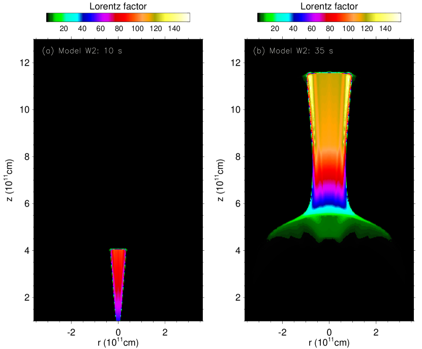
Figure 14: Lorentz factor for Model W2 at: (a) $t=10\,{\mathrm{s}}$ (left), and (b) $t=35\,{\mathrm{s}}$ (right) after jets start to propagate in the stellar wind. The initial opening angle is $3\arcdeg$. At $t=35\,{\mathrm{s}}$, the opening angle is $\sim 5\arcdeg$. This means there is little lateral expansion. Because the power and Lorentz factor decrease gradually after $10\,{\mathrm{s}}$, the tail of the jet experiences more lateral expansion, though not as much as in Model W1.

Some results are shown in Figs. 13 and 14. In both models, the Lorentz factor increases to more than 100 as the jet propagates in the stellar wind. There are very significant differences between Models W1 and W2. Although the initial opening angle in both is $3\arcdeg$, the opening angle at the head of the jet at $t=35\,{\mathrm{s}}$ is $15\arcdeg$ for Model W1 and $5\arcdeg$ for Model W2 (Fig. 15). In Model W1 the jet initially had a Lorentz factor of 10 and a large internal energy (93% of the total energy) leading to a large lateral expansion. In Model W2, the internal energy is less (67% of the total energy) and the Lorentz factor greater (50). One might argue that the final opening angle of the jet should be $\theta_{0}+1/\Gamma_{0}$ (see, e.g., Matzner 2002) in which case the final opening angles would be $8.7\arcdeg$ and $4.1\arcdeg$ for Models W1 and W2, respectively. Our larger angles correctly reflect the dynamics of a differentially accelerating relativistic jet.

As the jet expands sideways, the velocity along its edge does not increase as rapidly in the radial direction as at the center. A small amount of material actually ends up, briefly, with a slower radial component. The conversion of internal energy to kinetic energy during this phase causes sideways expansion. It should be noted that the radial component of momentum still increases when the radial component of velocity decreases because the total Lorentz factor is increasing during the sideways expansion. The combined effect of these two processes is that a small amount of material ends up at larger angles than expected from $\theta_{0}+1/\Gamma_{0}$. In Model W1, because of its lower initial Lorentz factor and higher internal energy loading, this effect is more pronounced and the opening angle increases from $3\arcdeg$ to $>6\arcdeg$ during the first second. The effect becomes less important as the Lorentz factor grows. In contrast, the final opening angle in Model W2 is only slightly larger than $\theta_{0}+1/\Gamma_{0}$ because of its higher initial Lorentz factor and lower internal energy loading. In order to test whether this large sideways expansion is due to low numerical resolution, we ran two higher resolution tests for Model W1. Finer grids (up to 3.3 times the original resolution of Model W1) were run for the same conditions. In one of the tests, the density of stellar wind was also increased by two orders of magnitude. These studies demonstrated that the resolution was already high enough to ensure the numerical viscosity contributed very little to the sideways expansion but are somewhat sensitive to the density of stellar wind (Fig. 16). Because of sideways expansion, the energy flux far off axis in Model W1 is small but not zero. In Model W2, the profile of energy flux is more uniform and has a sharper edge. In both cases the Lorentz factor profile is flat inside the jet in both models.

At later times, 10 to 20 seconds after the jet was initiated outside of the star, the energy deposition rate and Lorentz factor were gradually turned off as described previously. As a result, the tail of the jet experiences much more lateral expansion. Although the details depend on exactly how the central engine shuts down, it is natural that the jet should go a period of gradual decline rather than abruptly shutting off. Fig. 15 shows the energy flux and Lorentz factor at different locations for the two models. Mildly relativistic material is ejected at large angles. At the end of our simulations, the jets have two components: a core with high Lorentz factor and a wide tail with low Lorentz factor. In Model W1, the core has a rather flat energy flux profile inside $\sim 3\arcdeg$ and a rapidly decreasing energy flux profile extended to $\sim 15\arcdeg$. There is also a moderate relativistic ($\Gamma\sim 10$) tail outside the high Lorentz factor core. The Lorentz factor of the core is about $60-100$, but it has not reached its saturated value and is expected to become $\sim 150$ because of the remaining internal energy. In Model W2, the jet has a narrow core of $\sim 5\arcdeg$ with a very flat energy flux profile. It also contains moderately relativistic material outside the high Lorentz factor core. The implications for GRBs will now be discussed.

4 OBSERVATIONAL IMPLICATIONS

4.1 Beaming

Our special relativistic calculations show, as did Aloy et al. (2000), that a jet originating near the center of a collapsing massive star will emerge with an opening angle $\lesssim 5$ degrees. This result is relatively insensitive to the initial opening angle. Further expansion occurs after the jet has already emerged from the star. Depending on its Lorentz factor and internal energy loading at breakout, the final opening can be smaller than 5 degrees, or more than 15 degrees. This suggests that gamma-ray bursts can have a wide range of opening angle, and can be beamed to less than 1% of the sky with obvious implications for the requisite GRB energy and event rate.

4.2 GRB Light Curves

For a typical total energy in relativistic matter ($\Gamma>$ a few) of $\sim 3\times 10^{51}\,{\mathrm{erg}}$ (Frail et al., 2001; Freedman & Waxman, 2001), and an assumed Lorentz factor, $\Gamma\gtrsim 100$ (Lithwick & Sari, 2001), the mass within the GRB-producing beam is $\sim 10^{-5}\,M_{\sun}$, or about 1000 times less than that within the same solid angle in the precollapse star. In order to make a GRB using a jet launched from the stellar center, this stellar matter must be pushed aside. The matter shoved aside has two consequences. First, its lateral motion initiates a shock wave that moves round the star converging on the equator and exploding at least the outer part of the star as a supernova. Second, some of the material is swept back creating the cocoon of the jet. Instabilities between the cocoon and jet beam modulate the flow leading to a variable Lorentz factor. It is even possible that the jet might be temporarily clogged and reopened by the flow.

In this fashion, the variable Lorentz factor needed for the internal shock model for GRBs is generated. Light curves having very complex temporal behavior can result in situations where the central engine produced only a jet with constant power. The converse is also true. Short term time structure (less than the jet transit time through the star or about $5\,{\mathrm{s}}$) of the central engine may be erased as the jet passes through the reverse shock. If the variability of the engine itself is visible at all, it may only be at very late times when the star has exploded.

Our calculations show significant variation in the Lorentz factor of the emergent jet (Figs. 4, 5, 6 and 10). We suspect these variations may be larger in calculations with higher resolution, and in three dimensions.

Our model also suggests that the variability of GRB light curves may evolve with time. Though it takes awhile, of order a minute, for the star to explode away from the jet opening its channel appreciably, the Kelvin-Helmholtz instabilities should decrease with time. This implies that GRB variability may also decrease with time. A narrower jet experiences more instabilities and therefore the GRB is more variable. For a given total energy input at the bottom, a narrower jet also carries more energy per solid angle. Perhaps this might help to explain the observed correlation between luminosity and variability (Fenimore & Ramirez-Ruiz, 2000; Reichart et al., 2001).

4.3 A Unified Model For High Energy Transients

According to the “Unified Model” for active galactic nuclei (e.g., Antonucci 1993), one sees a variety of phenomena depending upon the angle at which a standard source is viewed. These range from tremendously luminous blazars, thought to be jets seen on axis, to narrow line radio galaxies and Type 2 Seyferts thought to be similar sources seen edge on. Given that an accreting black hole and relativistic jet may be involved in both, it is natural to seek analogies with GRBs.

In the equatorial plane of a collapsar - the common case - probably little more is seen than an extraordinary supernova. Along the axis, one sees an ordinary GRB, but there may also be interesting phenomena at intermediate angles. The calculations presented here clearly show that the edges of jets are not discontinuous surfaces. Moving off axis, one expects and calculates a smooth decline in the Lorentz factor and energy of relativistic ejecta. These low energy wings with moderate Lorentz factor come about in four ways. First, the jet that breaks out still has a lot of internal energy. Expansion of this material in the co-moving frame leads to a broadening of the jet. As a result a small amount of material with low energy ends up moving with intermediate Lorentz factors - say 10 - 30 and at angles up to several times that of the main GRB-producing jet. Second, as the star explodes from around the jet, the emerging beam opens up. Even at constant total power, the power per solid angle will decline as this channel broadens. Third, the jet is surrounded by a hot mildly relativistic cocoon. This material has low energy and low Lorentz factor. It can expand to large angles. Fourth, and potentially most important, the jet can continue with a declining total power for a long time. It is natural that the Lorentz factor of the emerging jet decline as well. A hot jet emerging with lower Lorentz factor will expand to larger angles (§ 3.3). As a consequence of the spreading of the jet, a large region of the sky, much larger than that which sees the main GRB, will see a hard transient with less power, lower Lorentz factor, and perhaps coming from an external shock instead of internal ones.

We have speculated for some time now (Woosley, Eastman, & Schmidt, 1999; Woosley & MacFadyen, 1999; Woosley, 2000, 2001) that these ordinary bursts seen off axis might appear as hard x-ray transients of one sort or another. We have identified them with GRB 980425 and with the class of hard x-ray flashes reported by Heise et al. (2001). These are not ordinary high $\Gamma$ jets seen just beyond a sharp edge (Ioka & Nakamura, 2001). The events are made by matter moving toward us.

4.4 Breakout Transients and Short Hard Bursts

The breakout of the jet and its interaction with the stellar wind will surely lead to some sort of “precursor” event. In fact, it is possible that this event could, in some cases, dominate the display.

The total energy in a short hard GRB (SHB) is, on the average, about 1/50 that of a long-soft burst (LSB). If the total gamma-ray energy of the latter averages $3\times 10^{50}\,{\mathrm{erg}}$, then SHBs at the same distance have gamma-ray energy, including the effects of beaming, of $\sim 10^{49}\,{\mathrm{erg}}$, or $\sim 3\times 10^{51}\,{\mathrm{erg}}$ in equivalent isotropic energy.

Our present calculations lack adequate resolution at the surface of the star to follow shock breakout with any accuracy. They also have not been followed sufficiently long to see the interaction of the leading head of the jet with the circumstellar medium. However, we do focus approximately $5\times 10^{51}\,{\mathrm{erg}}$ on only 1/800 of the stellar surface (for a fiducial opening half-angle of 4 degrees and a jet that takes $5\,{\mathrm{s}}$ to exit the star). This corresponds to an equivalent isotropic energy of $\sim 4\times 10^{54}\,{\mathrm{erg}}$. For their fiducial model with total isotropic energy $5\times 10^{54}\,{\mathrm{erg}}$, Tan, Matzner & McKee (2001) calculate about $3\times 10^{51}\,{\mathrm{erg}}$ is accelerated to Lorentz factor $\Gamma>40$. It may be that a larger amount of material is carried along by the leading edge of the jet as it expands and accelerates outside the star (see also Waxman & Mészáros 2002) if the lateral expansion of the “plug” cannot keep pace with the radial expansion of the jet.

Material having $3\times 10^{51}\,{\mathrm{erg}}$ in kinetic energy and $\Gamma\sim 40$, has a mass $\sim 4\times 10^{-5}$ $M_{\sun}$ which will decelerate after running into $10^{-6}\,M_{\sun}$. If the mass loss rate of the star during its last days was $10^{-4}\,M_{\sun}\,{\mathrm{yr}}^{-1}$ and the velocity $10^{8}\,{\mathrm{cm}}\,{\mathrm{s}}^{-1}$, this deceleration will occur within $3\times 10^{13}\,{\mathrm{cm}}$ or $1000\,{\mathrm{s}}$ in the lab frame. The duration of the burst is shortened by $\Gamma^{-2}$ to be less than a second, that is it may be a short one. But why then don’t we see such short hard precursors in all GRBs and how can one get short hard bursts in isolation?

The absence of SHBs in LSBs could, to some extent, be semantic, If the burst continues, a spike at the beginning may be counted as part of a long burst. But what about the converse problem - SHBs seen in isolation? The relative brightness of the breakout burst to the subsequent burst depends on many factors - the circumstellar density, the total energy of the jet, the variation of its Lorentz factor (especially critical in the internal shock model), and the mass of the star. This is especially so since SHBs could be made by external shocks and LSBs by internal shocks. So it may be, occasionally, that the breakout burst is an order of magnitude brighter (in flux, if not fluence) than the ensuing long burst. Of course, not all SHBs need to be produced this way and other models like merging neutron stars remain viable.

This possibility suggests that a careful search for postburst activity might be productive in SHBs. Preliminary results by Connaughton (2002) are suggestive of continuing postburst emission on a time scale not unlike that of LSBs, but are not sufficiently sensitive for a detailed comparison.

4.5 Post-burst Phenomenology

After the main burst is over, accretion will continue at a decaying rate. The lateral shock launched by the jet starts at the pole and wraps around the star, but does not reach into the origin at the equator. One may envision an angle-dependent “mass cut”. Consequently, some reservoir of matter remains to be accreted at late time. This accretion occurs at a rate governed by the viscosity of the residual disk and the free fall time of material farther out not ejected in the supernova. MacFadyen, Woosley, & Heger (2001) and Chevalier (1989) estimate the accretion rate from fall back to be $\sim 3\times 10^{-6}t_{4}^{-5/3}\,M_{\sun}\,{\mathrm{s}}^{-1}$. Here $t_{4}$ is the elapsed time since core collapse in units of $10^{4}\,{\mathrm{s}}$. Given the slow rate, the disk that forms is not neutrino dominated and there may be considerable high velocity flow from its surface (MacFadyen & Woosley, 1999; Narayan, Piran, & Kumar, 2001). That outflow will still be jet-like in nature since the equatorial plane is blocked by the disk and its energy will be $\sim 5\times 10^{46}t_{4}^{-5/3}\epsilon_{-2}\,{\mathrm{erg}}\,{\mathrm{s}}^{-1}$ where $\epsilon_{-2}=\epsilon/10^{-2}$ is the efficiency for converting rest mass into outflow kinetic energy measured in percent. This is comparable to the energy in x-ray afterglows and might be important for producing the emission lines reported in some bursts (Rees & Meszaros, 2000; Mészáros & Rees, 2001; McLaughlin et al., 2002) and for providing an extended tail of hard emission in the GRB itself.

As a consequence of this continuing outflow, the polar regions of the supernova made by the GRB remain evacuated and the photosphere of the object resembles an ellipse seen along its major axis but with conical sections removed along the axis. An observer can see deeper into the explosion than they could have without the operation of the jet’s “afterburner”.

5 FUTURE WORK

The present study, and its precursors by MacFadyen & Woosley (1999) and Aloy et al. (2000), have shown the critical role of the jet-star interaction in producing the observable properties of GRBs. Further work will be needed though to confirm the validity of the present results and add strength to some of the model’s more speculative aspects (§ 4).

First, it is important to repeat our calculations in three dimensions. Use of two dimensions imposes a rotational symmetry that makes it difficult for instabilities to deflect the beam. It may be that jets which maintain a stable focus here in 2D will waiver and even disperse in 3D. In any case, the Kelvin-Helmholtz instabilities may behave differently. Fortunately the computational requirements are not too extreme and such a calculation can be carried out in the near future.

Second, our jet needs to be studied with higher resolution. One can do that using cylindrical coordinates and a smaller range of radii. Again, we need to know the nature of the relativistic Kelvin-Helmholtz instability better.

The emergence of the jet and its immediate interaction with the circumstellar medium needs further examination, especially in a calculation that finally resolves the stellar surface at breakout and includes the jet cocoon as well as its core (see also Ramirez-Ruiz et al. 2002).

Finally, we are interested in the long term evolution of the jet and the star it is exploding. How much of the star remains to accrete even after the initial shock from the jet has wrapped around the star? How will the object appear, not seconds, but hours and days after the burst? How does this relate to the possibility of x-ray lines being detected in GRB afterglows.

Calculations to address all of these issues are underway.

Table 1: Parameters of Models for Jet Propagation inside Star

	$\dot{E}$	$\theta_{0}$
Model	($10^{51}\,{\mathrm{erg}}\,{\mathrm{s}}^{-1}$)	(degree)	$\Gamma_{0}$	$f_{0}$
JA	1.0	20	50	0.33
JB	1.0	5	50	0.33
JC	0.3	10	5	0.025

Table 2: Energies at Breakout

	$t_{\mathrm{b}}$	$E_{\mathrm{inj}}$	$E_{1}$	$E_{2}$	$E_{3}$	$E_{4}$	$E_{\mathrm{sn}}$
Model	(${\mathrm{s}}$)	($10^{51}\,{\mathrm{erg}}$)	($10^{51}\,{\mathrm{erg}}$)	($10^{51}\,{\mathrm{erg}}$)	($10^{51}\,{\mathrm{erg}}$)	($10^{51}\,{\mathrm{erg}}$)	($10^{51}\,{\mathrm{erg}}$)
JA	6.9	13.8	9.8	2.6	0.7	4.3	6.2
JB	3.3	6.6	3.6	0.4	0.1	4.9	1.2
JC	5.5	3.3	7.4	0.3	0.2	1.6	1.2

Table 3: Total Energies at End of Computation

	$T$	$E_{\mathrm{t}}$	$E_{\mathrm{w}}$	$E_{\mathrm{j}}$
Model	(${\mathrm{s}}$)	($10^{51}\,{\mathrm{erg}}$)	($10^{51}\,{\mathrm{erg}}$)	($10^{51}\,{\mathrm{erg}}$)
JA	21.8	43.6	8.5	35.1
JB	10.0	20.0	1.3	18.7
JC	15.0	9.0	1.7	7.3

Table 4: Parameters of Models for Jet Propagation in the Stellar Wind

	$\dot{E}$	$\theta_{0}$
Model	($10^{50}\,{\mathrm{erg}}\,{\mathrm{s}}^{-1}$)	(degree)	$\Gamma_{0}$	$f_{0}$
W1	8	3	10	0.06
W2	8	3	50	0.33

Figure 4: Pressure, density, Lorentz factor, and ratio of internal energy density to total energy density as a function of radius along the polar axis for Model JA. Different lines are for different times: $t=0.0\,{\mathrm{s}}$ (dash-dotted line), $t=2.0\,{\mathrm{s}}$ (dashed line), $t=8.0\,{\mathrm{s}}$ (dotted line), and $t=20.0\,{\mathrm{s}}$ (solid line). Pressure and density are measured in the local rest frame whereas energy density is measured in the laboratory frame. Fluctuations of all fluid variables are seen in the shocked region due to the complex flow patterns (Fig. 1). In the unshocked region, the flow is steady, reflecting the constancy of the injected jet. The total energy density here is the sum of internal energy and kinetic energy, not including the rest mass energy. In the unshocked region, the thermal energy of beam material is converted into kinetic energy by adiabatic expansion. At the outer boundary of the unshocked region, most of the kinetic energy is converted back into thermal energy by shock dissipation. At the head of the jet, the fraction of thermal energy decreases as the unshocked stellar gas is shocked and its kinetic energy increases.

Figure 5: Pressure, density, Lorentz factor, and the ratio of internal energy density to total energy density as a function of radius along the polar axis for Model JB. Different lines are for different times: $t=0.0\,{\mathrm{s}}$ (dash-dotted line), $t=1.0\,{\mathrm{s}}$ (dashed line), $t=4.0\,{\mathrm{s}}$ (dotted line), and $t=10.0\,{\mathrm{s}}$ (solid line). The head of unshocked region at $4.0\,{\mathrm{s}}$ lags behind the head of unshocked region at $1.0\,{\mathrm{s}}$ because of mixing among stellar medium, the cocoon, and the jet beam. See also Figs. 4 and 2.

Figure 6: Pressure, density, Lorentz factor, and the ratio of internal energy density to total energy density as a function of radius along the polar axis for Model JC. Different lines are for different times: $t=0.0\,{\mathrm{s}}$ (dash-dotted line), $t=2.0\,{\mathrm{s}}$ (dashed line), $t=5.0\,{\mathrm{s}}$ (dotted line), and $t=15.0\,{\mathrm{s}}$ (solid line). See also Figs. 4 and 3.

Figure 8: Lorentz factor vs. polar angle for: (a) Model JA (top) at $t=12.0\,{\mathrm{s}}$, (b) Model JB (middle) at $t=8.0\,{\mathrm{s}}$, and (c) Model JC (bottom) at $t=10.0\,{\mathrm{s}}$. These times are after breakout for the three models. Different lines are for several radii in the star: $r=2.1\times 10^{8}\,{\mathrm{cm}}$ (solid lines), $r=8.2\times 10^{9}\,{\mathrm{cm}}$ (dotted lines), $r=3.1\times 10^{10}\,{\mathrm{cm}}$ (dashed lines), and $r=8.0\times 10^{10}\,{\mathrm{cm}}$ (dash dotted lines). The dash multi-dotted lines are for: (a) Model JA (top) at $r=2.1\times 10^{10}\,{\mathrm{cm}}$, (b) Model JB (middle) at $r=1.8\times 10^{9}\,{\mathrm{cm}}$, and (c) Model JC (bottom) at $r=3.0\times 10^{9}\,{\mathrm{cm}}$. These locations are near the ends of the unshocked low-pressure and highly relativistic funnels. The jet has a high Lorentz factor inside the funnel and a mild Lorentz factor outside. The radius of the star is $8.0\times 10^{10}\,{\mathrm{cm}}$. The jets are very narrowly beamed as they pass through the star. The initial opening angles are $20\arcdeg$, $5\arcdeg$, and $10\arcdeg$ for Models JA, JB, and JC, respectively.

Figure 9: Energy flux at $9\times 10^{10}\,{\mathrm{cm}}$ for Models JA (top), JB (middle) and JC (bottom) after breakout. Here energy means total energy, including both kinetic and internal. Different lines are for different times: (a) $t=8.00\,{\mathrm{s}}$ (solid line), $t=12.00\,{\mathrm{s}}$ (dotted line), $t=16.00\,{\mathrm{s}}$ (dashed line), and $t=21.85\,{\mathrm{s}}$ (dash dotted line); (b) $t=4.00\,{\mathrm{s}}$ (solid line), $t=6.00\,{\mathrm{s}}$ (dotted line), $t=8.00\,{\mathrm{s}}$ (dashed line), and $t=10.00\,{\mathrm{s}}$ (dash dotted line); (c) $t=6.50\,{\mathrm{s}}$ (solid line), $t=9.00\,{\mathrm{s}}$ (dotted line), $t=12.00\,{\mathrm{s}}$ (dashed line), and $t=15.00\,{\mathrm{s}}$ (dash dotted line). In Model JA, the jet is “hollow”. In Models JB and JC, the energy flux is high in the middle. The radius of the star is $8\times 10^{10}\,{\mathrm{cm}}$.

Figure 10: Lorentz factor vs. time for: (a) Model JA, (b) Model JB, and (c) Model JC. Solid lines show current Lorentz factor of material on the axis at edge of our computational grid, $r=9\times 10^{11}\,{\mathrm{cm}}$. Dotted lines indicate the estimated terminal Lorentz factor if all internal energy is converted into kinetic energy.

Figure 11: Power of the relativistic jets at $9\times 10^{10}\,{\mathrm{cm}}$ for: Models JA (solid line), JB (dashed line), and JC (dotted line). This power includes both kinetic and internal energy fluxes calculated at the laboratory frame for material which has a Lorentz factor greater than 10. Time has been modified to show the three models together. The beginning of the solid line for Model JA is at $7\,{\mathrm{s}}$; the beginning of the dashed line for Model JB is at $3\,{\mathrm{s}}$; the beginning of the dotted line for Model JC is at $5\,{\mathrm{s}}$. Note that the energy flux increases very rapidly when the jet arrives at the surface.

Figure 12: Energy deposition rate (top), Lorentz factor (middle), and ratio of kinetic energy density to total energy density (bottom) of injected jet in Model W1 vs. time. Here, the energy deposition rate and the total energy density, which are measured in the laboratory frame, do not include the rest mass energy. This shows the history of injected jet in Model W1. During the first 10 seconds, a constant jet is injected in the stellar wind (Table 4). From 10 to 20 seconds, the jet energy decays. After 20 seconds, an outflow (zero gradient) boundary condition is used at the low z boundary. The recipe for the decaying jet in Model W2 is similar.

Figure 15: Density, energy flux, and Lorentz factor vs. angle for: (a) Model W1 and (b) W2. Here “density” is the local rest mass density and “energy” is the total energy measured in the lab frame, both kinetic and internal. The time is $35\,{\mathrm{s}}$ after the jets break out. Different lines show results at different locations: $r=5.5\times 10^{11}\,{\mathrm{cm}}$ (dashed lines), $r=7.5\times 10^{11}\,{\mathrm{cm}}$ (dotted lines), and $r=10^{12}\,{\mathrm{cm}}$ (solid lines). Here, $r$ is the distance to the center of the star. The angle is measured relative to the polar axis starting at the center of the star. The opening angles at $t=35\,{\mathrm{s}}$ are $\sim 15\arcdeg$ and $\sim 5\arcdeg$, for Models W1 and W2, respectively.

Figure 16: Density and Lorentz factor vs. angle for three calculations of Model W1 using different resolutions and stellar wind densities. Here, the density is the local rest mass density. The angle is measured relative to the polar axis starting at the center of the star. The three simulations used: (1) higher resolution and normal stellar wind density (solid lines); (2) normal resolution and normal stellar wind density (dotted lines); and (3) higher resolution and higher stellar wind density (dashed lines). The time is at $t=10\,{\mathrm{s}}$. These lines all show results at $r=3.95\times 10^{11}\,{\mathrm{cm}}$ where $r$ is the distance to the center of the star.

References

- Aloy et al. (1999) Aloy, M. A., Ibáñez, J. M., Martí, J. M., & Müller, E. 1999, ApJS, 122, 151
- Aloy et al. (2000) Aloy, M. A., Müller, E., Ibáñez, J. M., Martí, J. M., & MacFadyen, A. I. 2000, ApJ, 531, L119
- Antonucci (1993) Antonucci, R. 1993, ARAA, 31, 473
- Blandford & Rees (1974) Blandford, R. D., & Rees, M. J. 1974, MNRAS, 169, 395
- Blinnikov, Dunina-Barkovskaya, & Nadyozhin (1996) Blinnikov, Dunina-Barkovskaya, & Nadyozhin 1996, ApJS, 106, 171
- Bloom et al. (1999) Bloom, J. S., Kulkarni, S. R., Djorgovski, S. G., Eichelberger, A. C., Cote, P., Blakeslee, J. P., Odewahn, S. C., Harrison, F. A., et al. 1999, Nature, 401, 453
- Bloom et al. (2002) Bloom, J. S., Kulkarni, S. R., Price, P. A., Reichart, D., Galama, T. J., Schmidt, B. P., Frail, D. A., Berger, E., et al. 2002, ApJ, 572, L45
- Bloom, Kulkarni, & Djorgovski (2002) Bloom, J. S., Kulkarni, S. R., & Djorgovski, G. 2002, AJ, 123, 1111
- Chevalier (1989) Chevalier, R. A. 1989, ApJ, 346, 847
- Connaughton (2002) Connaughton, V. 2002, ApJ, 567, 1028
- Fenimore & Ramirez-Ruiz (2000) Fenimore, E. E., & Ramirez-Ruiz, E. 2000, ApJ, submitted, astro-ph/0004176)
- Ferrari, Trussoni, & Zaninetti (1978) Ferrari, A., Trussoni, E., & Zaninetti, L. 1978, A&A, 64, 43
- Frail et al. (2001) Frail, D., et al. 2001, ApJ, 562, L55
- Freedman & Waxman (2001) Freedman, D. L., & Waxman, E. 2001, ApJ, 547, 922
- Galama et al. (1998) Galama, T. J., Vreeswijk, P. M., van Paradijs, J., Kouveliotou, C., Augusteijn, T., Bohnhardt, H., et al. 1998, Nature, 395, 670
- Galama et al. (2000) Galama, T. J., Tanvir, N., Vreeswijk, P. M., Wijers, R. A. M. J., Groot, P. J., Rol, E., van Paradijs, J., Kouveliotou, C. et al. 2000, ApJ, 536, 185
- Garnavich et al. (2002) Garnavich, P. M., et al. 2002, ApJ, submitted, astro-ph/0204234
- Heger, Langer, & Woosley (2001) Heger, A., Langer, N., & Woosley, S. E. 2001, ApJ, 528, 368
- Heger & Woosley (2002) Heger, A. & Woosley, S. E. 2002, in Proc. Woods Hole GRB meeting, ed. Roland Vanderspek, in press, astro-ph/0206005.
- Heise et al. (2001) Heise, J., in’t Zand, J., Kippen, R. M., Woods, P. M. 2001, GRBs in the Afterglow Era, eds. Costa, Frontera, & Hjorh, ESO Astrophysics Symposia, (Springer), 16
- Ioka & Nakamura (2001) Ioka, K., & Nakamura, T. 2001, ApJ, 554, L163
- Iwamoto et al. (1998) Iwamoto, K., et al. 1998, Nature, 395, 672
- Lithwick & Sari (2001) Lithwick, Y., & Sari, R. 2001, ApJ, 555, 540
- MacFadyen & Woosley (1999) MacFadyen, A. I., & Woosley, S. E. 1999, ApJ, 524, 262
- MacFadyen, Woosley, & Heger (2001) MacFadyen, A. I., Woosley, S. E., & Heger, A. 2001, ApJ, 550, 410
-
Martí & Müller (1999)
Martí, J. M., & Müller, E. 1999,
Living Reviews in Relativity,
http://www.livingreviews.org/Articles/Volume2/1999-3marti - Martí et al. (1997) Martí, J. M., Müller, E., Font, J. A., Ibáñez, J. M., & Marquina, A. 1997, ApJ, 479, 151
- Matzner (2002) Matzner, C. D. 2002, MNRAS, submitted, astro-ph/0203085
- McLaughlin et al. (2002) McLaughlin, G. C., Wijers, R. A. M. J., & Brown, G. E., & Bethe, H. A. 2002, ApJ, 567, 454
- Mészáros, Laguna, & Rees (1993) Mészáros, P., Laguna, P., & Rees, M. J. 1993, ApJ, 415, 181
- Mészáros & Rees (2001) Mészáros, P., & Rees, M. J. 2001, ApJ, 556, L37
- Narayan, Piran, & Kumar (2001) Narayan, R., Piran, T., & Kumar, P. 2001, ApJ, 557, 949
- Panaitescu & Kumar (2001) Panaitescu, A., & Kumar, P. 2001, ApJ,560, L49
- Price et al. (2002) Price, P. A., et al. 2002, ApJ, submitted, astro-ph/0208008
- Ramirez-Ruiz, Celotti, & Rees (2002) Ramirez-Ruiz, E., Celotti, A., & Rees, M. J. 2002, MNRAS, in press, astro-ph/0205108
- Rees & Meszaros (2000) Rees M. J., & Meszaros, P. 2000, ApJ, 545, L73
- Reichart (1999) Reichart, D. 1999, ApJ, 521, L111
- Reichart et al. (2001) Reichart, D. E., Lamb, D. Q., Fenimore, E. E., Ramirez-Ruiz, E., Cline, T. L., & Hurley, K. 2001, ApJ, 552, 57
- Tan, Matzner & McKee (2001) Tan, J. C., Matzner, C. D., & McKee, C. F. 2001, ApJ, 551, 946
- Waxman & Mészáros (2002) Waxman, E., & Mészáros, P. 2002, ApJ, in press, astro-ph/0206392
- Woosley, Eastman, & Schmidt (1999) Woosley, S. E., Eastman, R. G., & Schmidt, B. 1999, ApJ, 516, 788
- Woosley & MacFadyen (1999) Woosley, S. E. & MacFadyen, A. I. 1999, A&AS, 138, 499
- Woosley (2000) Woosley, S. E. 2000, GRBs, 5th Huntsville Symposium, eds. Kippen, Mallozzi, & Fishman, AIP, Vol 526, 555
- Woosley (2001) Woosley, S. E. 2001, GRBs in the Afterglow Era, eds. Costa, Frontera, & Hjorh, ESO Astrophysics Symposia, (Springer), 257