Helioseismology

Abstract

Oscillations detected on the solar surface provide a unique possibility for investigations of the interior properties of a star. Through major observational efforts, including extensive observations from space, as well as development of sophisticated tools for the analysis and interpretation of the data, we have been able to infer the large-scale structure and rotation of the solar interior with substantial accuracy, and we are beginning to get information about the complex subsurface structure and dynamics of sunspot regions, which dominate the magnetic activity in the solar atmosphere and beyond. The results provide a detailed test of the modeling of stellar structure and evolution, and hence of the physical properties of matter assumed in the models. In this way the basis for using stellar modeling in other branches of science is very substantially strengthened; an important example is the use of observations of solar neutrinos to constrain the properties of the neutrino.

Contents

toc

I Introduction

By the standards of astrophysics, stars are relatively well understood. Modelling of stellar evolution has explained, or at least accounted for, many of the observed properties of stars. Stellar models are computed on the basis of the assumed physical conditions in stellar interiors, including the thermodynamical properties of stellar matter, the interaction between matter and radiation and the nuclear reactions that power the stars. By following the changes in structure as the stars evolve through the fusion of lighter elements into heavier, starting with hydrogen being turned into helium, the models predict how the observable properties of the stars change as they age. These predictions can then be compared to observations. Important examples are the distributions of stars in terms of surface temperature and luminosity, particularly for stellar clusters where the stars, having presumably been formed in the same interstellar cloud, can be assumed to share the same age and original composition. These distributions are generally in reasonable agreement with the models; the comparison between observations and models furthermore provides estimates of the ages of the clusters, of considerable interest to the understanding of the evolution of the Galaxy. Additional tests, generally quite satisfactory, are provided in the relatively few cases where stellar masses can be determined with reasonable accuracy from the motion of stars in binary systems. Such successes give some confidence in the use of stellar models in other areas of astrophysics. These include studies of element synthesis in late stages of stellar evolution, the use of supernova explosions as ‘standard candles’ in cosmology, and estimates of the primordial element composition from stellar observations.

An important aspect of stellar astrophysics is the use of stars as physics laboratories. Since the basic properties of stars and their modeling are presumed to be relatively well established, one may hope to use more detailed observations to provide information about the physics of stellar interiors, to the extent that it is reflected in observable properties. This is of obvious interest: conditions in the interiors of stars are generally far more extreme, in terms of temperature and density, than achievable under controlled circumstances in terrestrial laboratories. Thus sufficiently detailed stellar data might offer the hope of providing information on the properties of matter under these conditions.

Yet in reality there is little reason to be complacent about the status of stellar astrophysics. Most observations relevant to stellar interiors provide only limited constraints on the detailed properties of the stars. Where more extensive information is becoming available, such as determinations of detailed surface abundances, the models often fail to explain it. Furthermore, the models are in fact extremely simple, compared to the potential complexities of stellar interiors. In particular, convection, which dominates energy transport in parts of most stars, is treated very crudely while other potential hydrodynamical instabilities are generally neglected. Also stellar rotation is rarely taken into account, yet could have important effects on the evolution. These limitations could have profound effects on, for example, the modeling of late stages of stellar evolution, which depend sensitively on the composition profile established during the life of the star.

The Sun offers an example of a star that can be studied in very great detail. Furthermore, it is a relatively simple star: it is in the middle of its life, with approximately half the original central abundance of hydrogen having been used, and, compared to some other stars, the physical conditions in the solar interior are relatively benign. Thus in principle the Sun provides an ideal case for testing the theory of stellar evolution.

In practice, the success of such tests was for a long time somewhat doubtful. Solar modeling depends on two unknown parameters: the initial helium abundance and a parameter characterizing the efficacy of convective energy transport near the solar surface. These parameters can be adjusted to provide a model of solar mass, matching the solar radius and luminosity at the age of the Sun. Given this calibration, however, the measured surface properties of the Sun provide no independent test of the model. Furthermore, two potentially severe problems with solar models have been widely considered. One, the so-called faint early Sun problem, resulted from the realization that solar models predicted that the initial luminosity of the Sun, at the start of hydrogen fusion, was approximately 70 per cent of the present value, yet geological evidence indicated that there had been no major change in the climate of the Earth over the past 3.5 Gyr (e.g., Sagan and Mullen, 1972). This change in luminosity is a fundamental effect of the conversion of hydrogen to helium and the resulting change in solar structure; thus the attempts to eliminate it resorted to rather drastic measures, such as suggestions for changes to the gravitational constant. As noted by Sagan and Mullen, a far more likely explanation is a readjustment of conditions in the Earth’s atmosphere to compensate for the change in luminosity. A more serious concern was the fact that attempts to detect the neutrinos created by the fusion reactions in the solar core found values far below the predictions. This evidently raised doubts about the computations of solar models, and hence on the general understanding of stellar evolution, and led to a number of suggestions for changing the models such as to bring them into agreement with the neutrino measurements.

The last three decades have seen a tremendous growth in our information about the solar interior, through the detection and extensive observation of oscillations of the solar surface. Analyses of these oscillations, appropriately termed helioseismology, have resulted in extremely precise and detailed information about the properties of the solar interior, rivaling or in some respects exceeding our knowledge about the interior of the Earth.

II Early history of helioseismology

The development of helioseismology has to a large extent been driven by observations. Hence in the following I provide an overview of the evolution of observations of solar oscillations. Discussions of the development of helioseismic inferences follow in later sections.

It is possible that the first indications of solar oscillations were detected by Plaskett (1916), who observed fluctuations in the solar surface Doppler velocity in measurements of the solar rotation rate. It was not clear, however, whether the fluctuations were truly solar or whether they were induced by effects in the Earth’s atmosphere. The solar origin of these fluctuations was established by Hart (1954, 1956). However, the first definite observations of oscillations of the solar surface were made by Leighton et al. (1962). They detected roughly periodic oscillations in local Doppler velocity with periods of around 300 s and a lifetime of at most a few periods. Strikingly, they noted the potential for using the observed period to probe the properties of the solar atmosphere. A confirmation of the initial detection of the oscillations was made by Evans and Michard (1962). The observations by Leighton et al. (1962) also led to the detection of convective motion on supergranular scales. As discussed in section X B, the study of solar oscillations and supergranulation has recently come together again.

Early observations of the five-minute oscillations were of short duration and limited spatial extent. With only such information, the oscillations were generally interpreted as local phenomena in the solar atmosphere, of limited spatial and temporal coherence, possibly waves induced by penetrating convection (e.g., Bahng and Schwarzschild, 1963). However, attempts at determining their structure were made by several authors, including Frazier (1968); through observations and Fourier transforms of the oscillations as a function of position and time, he could make power spectra as a function of wavenumber and frequency, showing some localization of power. Such observations indicated a less superficial nature of the oscillations, and inspired major theoretical advances in the understanding of their nature: Ulrich (1970) and Leibacher and Stein (1971) proposed that the observations resulted from standing acoustic waves in the solar interior. Such calculations were further developed by Wolff (1972) and Ando and Osaki (1975), who found that oscillations in the relevant frequency and wavenumber range may be linearly unstable. However, the definite breakthrough were the observations by Deubner (1975) which for the first time identified ridges in the wavenumber-frequency diagram, reflecting the modal structure of the oscillations. Similar observations were reported by Rhodes et al. (1977), who furthermore compared the frequencies with computed models to obtain constraints on the properties of the solar convection zone.

The year of 1975 was indeed the annus mirabilis of helioseismology. An important event was the announcement by H. A. Hill of the detection of oscillations in the apparent solar diameter (see Hill et al., 1976; Brown et al., 1978). This was the first suggestion of truly global oscillations of the Sun and immediately indicated the possibility of using such data to investigate the properties of the solar interior (e.g., Scuflaire et al., 1975; Christensen-Dalsgaard and Gough, 1976; Iben and Mahaffy, 1976; Rouse, 1977). Simultaneously, Brookes et al. (1976) and Severny et al. (1976) announced independent detections of a solar oscillation with a period of 160 min, with similarly interesting diagnostic potentials. Even though these detections have since been found to be of likely non-solar origin, they played a very important role as inspiration for the development of helioseismology.

(For the present author, the announcement by Hill was particularly significant. It took place at a conference in Cambridge in the Summer of 1975. I was engaged, with Douglas Gough, in modeling solar structure and oscillations, as part of an investigation of mixing induced by oscillations as a possible explanation of the solar neutrino problem. As a result, we had available solar models and programmes for computing their frequencies. Hill presented an observed spectrum and I was able, the following day, to compare it with frequencies computed for a model; the agreement was quite striking. It has since transpired that the observations had little to do with global oscillations of the Sun; and the model was surely far too crude for such a comparison. Even so, the event was a major personal turning point, directing my scientific efforts towards helioseismology.)

The next major observational step was the identification by Claverie et al. (1979) of modal structure of five-minute oscillations in Doppler-velocity observations in light integrated over the solar disk. Such observations are sensitive only to oscillations of the lowest spherical-harmonic degree, and hence these were the first confirmed detection of truly global modes of oscillations. The frequency pattern, with regularly spaced peaks, matched theoretical predictions based on the asymptotic theory of acoustic modes of high radial order (Christensen-Dalsgaard and Gough, 1980a; see also Section V C 3). Further observations, with much higher frequency resolution, were made from the Geographical South Pole during the austral summer 1979–80 (Grec et al., 1980); these resolved the individual multiplets in the low-degree spectrum and allowed a comparison between the frequency data, including also the so-called small frequency separation, and solar models. The structure of the frequency spectrum was analyzed asymptotically by Tassoul (1980). It was pointed out by Gough (1982) that the small separation was related to the curvature of sound speed in the solar core; thus it would, for example, provide evidence for mixing of material in the core (see Section V C 3).

The existence of oscillations in the five-minute range, both a low degree as detected by Claverie et al. (1979) and at high wavenumbers as found by Deubner (1975), strongly suggested a common cause (e.g., Christensen-Dalsgaard and Gough, 1982). The gap between these observations was filled by Duvall and Harvey (1983), who made detailed observations at intermediate degree. This also allowed a definite identification of the order of the modes, even at low degree, by establishing the connection with the high-degree modes for which the order could be directly determined. By providing a full range of modes these and subsequent observations opened the possibilities for detailed inferences of properties of the solar interior, such as the internal solar rotation (Duvall et al., 1984) and the sound speed (Christensen-Dalsgaard et al., 1985).

III Overall properties of the Sun

The Sun is unique amongst stars in that its properties are known with high precision. The product $GM_{\odot}$, where $G$ is the gravitational constant and $M_{\odot}$ is the mass of the Sun, is known with very high accuracy from planetary motion. Thus the factor limiting the accuracy of $M_{\odot}$ is the value of $G$; the commonly used value is $M_{\odot}=1.989\times 10^{33}\,{\rm g}$. The solar radius $R_{\odot}$ follows from the apparent diameter and the distance to the Sun. Most recent computations of solar models have used $R_{\odot}=6.9599\times 10^{10}\,{\rm cm}$ (Auwers, 1891). The solar luminosity $L_{\odot}$ is determined from satellite irradiance measurements, suitably averaged over the variation of around 0.1 % during the solar cycle (e.g., Willson and Hudson, 1991; Pap and Fröhlich, 1999); a commonly used value is $L_{\odot}=3.846\times 10^{33}\,{\rm erg}\,{\rm s}^{-1}$. Finally, the age of the Sun is obtained from age determinations for meteorites, combined with modeling of the formation history of the solar system (e.g., Guenther, 1989; Wasserburg, in Bahcall and Pinsonneault, 1995). Based on a careful analysis, Wasserburg estimated the age as $t_{\odot}=(4.566\pm 0.005)\times 10^{9}$ yr.

The composition of stellar matter is traditionally characterized by the relative abundances by mass $X$, $Y$ and $Z$ of hydrogen, helium and ‘heavy elements’ (i.e., elements heavier than helium). The solar surface composition can in principle be determined from spectroscopic analysis. In practice, the principle works for most elements heavier than helium; for elements with lines in the solar photospheric spectrum, abundances can be determined with reasonable precision, although often limited by uncertainties in the relevant basic atomic parameters and in the modeling of the solar atmosphere (e.g., Asplund et al., 2000b), as well as by blending with weak lines (e.g., Allende Prieto et al., 2001). The relative abundances so obtained are generally in good agreement with solar-system abundances as inferred from meteorites (e.g., Anders and Grevesse, 1989; Grevesse and Sauval, 1998). A striking exception is the abundance of lithium, which is lower by about a factor 150, relative to silicon, in the Sun than in meteorites. There have been suggestions that the beryllium abundance is lower also, but the most recent determinations seems to indicate that the solar beryllium abundance is similar to the meteoritic value (e.g., Balachandran and Bell, 1998). As discussed in Section XI these observations are of great interest in connection with investigations of solar internal structure and dynamics.

The noble gases, including helium, do not have lines in the photospheric spectrum as a result of the large excitation energies of the relevant atomic transitions. It is true that helium can be detected in the solar spectrum, but only through lines formed high in the solar atmosphere where conditions are complex and uncertain and a reliable abundance determination is therefore not possible. As a result, the solar helium abundance is not known from ‘classical’ observations. Typically, the initial abundance $Y_{0}$ by mass is used as a free parameter in solar-model calculations. On the other hand, spectroscopic data do provide a measure of the ratio $Z_{\rm s}/X_{\rm s}$ of the present surface abundances heavy elements and hydrogen; commonly used values are 0.0245 (Grevesse and Noels, 1993) and 0.023 (Grevesse and Sauval, 1998).

Solar surface rotation can be determined by following the motion of features on the solar surface (e.g., sunspots) as they move across the solar disk, or through Doppler measurements. The angular velocity $\Omega$ obtained from Doppler measurements, as a function of co-latitude $\theta$, can be fitted by the following relation

$${\Omega\over 2\pi}=451.5\,{\rm nHz}-65.3\,{\rm nHz}\,\cos^{2}\theta-66.7\,{\rm nHz}\,\cos^{4}\theta$$ (1)

(Ulrich et al., 1988), although there are significant departures from this relation, as well as variations with time (see also Section IX).

IV Solar structure and evolution

A ‘Standard’ solar models

As a background for the discussion of the helioseismically inferred information about the solar internal structure, it is useful briefly to summarize the principles of computation of ‘standard’ solar models. Such models are assumed to be spherically symmetric, ignoring effects of rotation and magnetic field. In that case, the basic equations of stellar structure can be written

$${{\rm d}p\over{\rm d}r} = -{Gm\rho\over r^{2}}\;,$$ (3)

$${{\rm d}m\over{\rm d}r} = 4\pi r^{2}\rho\;,$$ (4)

$${{\rm d}T\over{\rm d}r} = \nabla{T\over p}{{\rm d}p\over{\rm d}r}\;,$$ (5)

$${{\rm d}L\over{\rm d}r} = 4\pi r^{2}\left[\rho\epsilon-\rho{{\rm d}\over{\rm d}t}\left({u\over\rho}\right)+{p\over\rho}{{\rm d}\rho\over{\rm d}t}\right]\;.$$ (6)

Here $r$ is distance to the center, $p$ is pressure, $m$ is the mass of the sphere interior to $r$, $\rho$ is density, $T$ is temperature, $L$ is the flow of energy per unit time through the sphere of radius $r$, $\epsilon$ is the rate of nuclear energy generation per unit mass and time, and $u$ is the internal energy per unit volume. Also, the temperature gradient has been characterized by $\nabla={\rm d}\ln T/{\rm d}\ln p$ and is determined by the mode of energy transport. Where energy is transported by radiation, $\nabla=\nabla_{\rm rad}$, where the radiative gradient is given by

$$\nabla_{\rm rad}={3\over 16\pi a\tilde{c}G}{\kappa p\over T^{4}}{L(r)\over m(r)}\;;$$ (7)

here $\tilde{c}$ is the speed of light, $a$ is the radiation density constant and $\kappa$ is the opacity, defined such that $1/(\kappa\rho)$ is the mean free path of a photon. In regions where $\nabla_{\rm rad}$ exceeds the adiabatic gradient $\nabla_{\rm ad}=(\partial\ln T/\partial\ln p)_{s}$, the derivative being taken at constant specific entropy $s$, the layer becomes unstable to convection. In that case energy transport is predominantly by convective motion; as discussed below, the detailed description of convection is highly uncertain.

Energy generation in the Sun results from the fusion of hydrogen into helium. The net reaction can be written as

$$4\,{\rm{}^{1}H}\rightarrow\,{\rm{}^{4}He}+2{\rm e}^{+}+2\nu_{\rm e}\;,$$ (8)

satisfying the constraints of conservation of charge and lepton number. Here the positrons are immediately annihilated, while the electron neutrinos escape the Sun essentially without reacting with matter and therefore represent an immediate energy loss. The actual path by which this net reaction takes place involves different sequences of reactions, depending on the temperature (for details, see for example Bahcall, 1989). These reactions differ substantially in the neutrino energy loss and hence in the energy actually available to the star.

The change in composition resulting from Eq. (8) largely drives solar evolution. Until fairly recently, ‘standard’ solar model calculations did not include any other effects that changed the composition. However, Noerdlinger (1977) pointed out the potential importance of diffusion of helium in the Sun. Strong evidence for the importance of diffusion and settling has since come from helioseismology (see Section VII A) and these processes are now generally included in the calculations. Specifically, the rate of change of the hydrogen abundance is written

$${\partial X\over\partial t}={\cal R}_{\rm H}+{1\over r^{2}\rho}{\partial\over\partial r}\left[r^{2}\rho\left(D_{\rm H}{\partial X\over\partial r}+V_{\rm H}X\right)\right]\;;$$ (9)

here ${\cal R}_{\rm H}$ is the rate of change in the hydrogen abundance from nuclear reactions, $D_{\rm H}$ is the diffusion coefficient and $V_{\rm H}$ is the settling speed. Similar equations are of course satisfied for the abundances of other elements. In Eq. (9), the term in $D_{\rm H}\partial X/\partial r$ tends to smooth out composition gradients, whereas the term in the settling velocity leads to separation, hydrogen rising towards the surface and heavier elements including helium sinking towards the interior.

The basic equations of stellar structure and evolution, Eqs (‡ ‣ IV A) and (9), are relatively simple; also, the numerical techniques for solving them are well established and well tested in the case of solar models. However, the apparent simplicity hides a great deal of complexity, often combined under the heading of ‘microphysics’. To complete the equations, their right-hand sides must be expressed in terms of the basic variables $\{p,m,T,L,X_{i}\}$, where $X_{i}$ denotes the abundances of the relevant elements. This requires expressions for the density $\rho$ and other thermodynamic variables, for the opacity $\kappa$, for the energy generation rate $\epsilon$ and the rates of change of composition ${\cal R}_{i}$, as well as for the diffusion and settling coefficients. At the level of precision required for solar modeling, each of these components involves substantial physical subtleties. The thermodynamic quantities are obtained from an equation of state, which as a minimum requirement (although not always met) must satisfy thermodynamic consistency. Two conceptually very different formulations are in common use: one is the so-called ‘chemical picture’ where the equation of state is based on an expression for the free energy of a system consisting of atoms, ions, etc., containing the relevant physical effects; the second is the ‘physical picture’, which assumes as building blocks only fundamental particles (nuclei and electrons), and treats density effects by means of a systematic expansion (for reviews, see for example Däppen, 1998; Däppen and Guzik, 2000). A representative and commonly used example of the chemical picture is the so-called MHD equation of state (Mihalas et al., 1988). The physical picture has been implemented by the OPAL group (Rogers et al., 1996). In the opacity calculation the detailed distribution of the atoms on ionization and excitation states must be taken into account, obviously requiring a sufficiently accurate equation of state (see Däppen and Guzik, 2000). The most commonly used opacity tables are those of the OPAL group (Iglesias and Rogers, 1996). Computation of the energy generation and composition changes obviously requires nuclear cross sections, the determination of which is greatly complicated by the low typical reaction energies relevant to stellar interiors; recently, two major compilations of nuclear parameters have been published by Adelberger et al. (1998) and Angulo et al. (1999). Additional complications result from the partial screening of the Coulomb potential of the reacting nuclei by the stellar plasma; the so-called weak-screening approximation (Salpeter, 1954) is still in common use. Expressions for the diffusion and settling coefficients have been provided by, for example, Michaud and Proffitt (1993) and Thoul et al. (1994).

In the Sun, convection occurs in the outer about 29% of the solar radius; this is visible on the solar surface in the form of motion and other fluctuations in the so-called granulation and supergranulation. In the convectively unstable regions, modeling requires a relation to determine the convective energy transport from the local structure; particularly important is the superadiabatic gradient, i.e., the difference between the actual temperature gradient $\nabla$ and the adiabatic value $\nabla_{\rm ad}$, which controls both the dynamics of the convective motion and the net energy transport. In model calculations this relation is typically obtained from simple recipies, and characterized by one or more parameters that determine convective efficacy. A characteristic example is the mixing-length treatment (Böhm-Vitense, 1958), parametrized by the mixing-length parameter $\alpha_{\rm c}$ which measures the mean free path of convective eddies in units of the local pressure scale height. Also, it is common to neglect the dynamical effects of convection, generally described as a turbulent pressure. In most of the solar convection zone, convection is so efficient that the actual temperature gradient is very close to the adiabatic value. Near the surface, however, where the density is low, a fairly substantial superadiabatic gradient is required to transport the energy. The effect of the parametrization of the convection treatment through, e.g., $\alpha_{\rm c}$ is to control the degree of superadiabaticity and hence, effectively, the adiabat of the nearly adiabatic part of the convection zone (cf. Gough & Weiss, 1976).

A more realistic description of the uppermost part of the convection zone is possible through detailed three-dimensional and time-dependent hydrodynamical simulations, taking into account radiative transfer in the atmosphere (e.g., Stein and Nordlund, 1998a). Such simulations successfully reproduce the observed surface structure of solar granulation (e.g., Nordlund and Stein, 1997), as well as detailed profiles of lines in the solar radiative spectrum, without the use of parametrized models of turbulence (Asplund et al., 2000a). The simulations only cover a very small fraction of the solar radius, and are evidently far too time-consuming to be included in general solar modeling. Rosenthal et al. (1999) extrapolated an averaged simulation through the adiabatic part of the convection zone by means of a model based on the mixing-length description, demonstrating that the adiabat predicted by the simulation was essentially consistent with the depth of the solar convection zone as determined from helioseismology (see Section VII). Also, Li et al. (2002) developed an extension of mixing-length theory, including effects of turbulent pressure and kinetic energy, based on numerical simulations of near-surface convection.

FIG. 1.: Hydrogen mass fraction $X$ as a function of fractional radius in a model of the present Sun (Model S of Christensen-Dalsgaard et al., 1996). The insert shows details of the behavior near the base of the convection zone.

The computation of a model of the present Sun typically starts from the so-called zero-age main sequence, where the model can be assumed to be of uniform composition, with nuclear reactions providing the energy output; however, models have also been computed starting during the earlier phase of gravitational contraction (e.g., Morel et al., 2000). The model is characterized by the mass (generally assumed to be constant during the evolution) and the initial composition, specified by the abundances $X_{0}$, $Y_{0}$ and $Z_{0}$. In addition, parameters characterizing convective energy transport, such as the mixing-length parameter $\alpha_{\rm c}$, must be specified. The model at the age of the present Sun must match the present solar radius and luminosity, as well as the observed ratio $Z_{\rm s}/X_{\rm s}$ of the abundance of heavy elements to hydrogen at the surface. This is achieved by adjusting $\alpha_{\rm c}$ and $Y_{0}$, which largely control the radius and luminosity, and the initial heavy-element abundance $Z_{0}$.

To illustrate some properties of models of the present Sun, Fig. 1 shows the hydrogen-abundance profile $X$. The abundance is uniform in the outer convection zone, extending from the surface to $r=0.711R$, which is fully mixed; as a result of helium settling, $X$ has increased by about 0.03 relative to its initial value of 0.709. Just below the convection zone, helium settling has caused a sharp gradient in the hydrogen abundance. In the inner parts of the model the hydrogen abundance has been reduced due to nuclear fusion. Detailed tables of model quantities, from a slightly different calculation, were provided by Bahcall and Pinsonneault (1995).

B Solar neutrinos

As indicated in Eq. (8), hydrogen fusion in the Sun unavoidably produces electron neutrinos. It is easy to estimate, from the solar energy flux, that the total flux of solar neutrinos at the Earth is around $7\times 10^{10}\,{\rm cm}^{-2}\,{\rm s}^{-1}$. This depends little on the details of the nuclear reactions in the solar core, as long as the solar energy output derives solely from nuclear reactions. However, the energy spectrum of the neutrinos depends sensitively on the branching between the various reactions. This is particularly true of the highest-energy neutrinos, which are produced by a relatively rare and very temperature-sensitive reaction. This is of crucial importance to attempts to detect neutrinos from the Sun.

A detailed description of the issues related to solar neutrinos, including their detection, was given by Bahcall (1989). More recent reviews have been provided by, for example, Haxton (1995), Castellani et al. (1997), Kirsten (1999), and Turck-Chièze (1999). Until recently, three classes of experiments had been carried out to detect solar neutrinos. The first experiment, where the $\nu_{\rm e}$ reacted with chlorine, was established by R. Davis in the Homestake Gold Mine, South Dakota, and yielded its initial results in 1968 (Davis et al., 1968), providing an upper limit on the capture rate of 3 SNU (Solar Neutrino Units; 1 SNU corresponds to $10^{-36}$ reactions per target atom per second). This was substantially below the expected flux (e.g., Bahcall, Bahcall & Shaviv, 1968). The latest average measured value is ${\rm 2.56\pm 0.16(statistical)\pm 0.16(systematic)}$ SNU (Cleveland et al., 1998); this is to be compared to typical model predictions of around 8 SNU (e.g., Bahcall et al., 2001; Turck-Chièze et al., 2001a).

This experiment is most sensitive to high-energy neutrinos, and hence the predictions depend on the solar central temperature to a high power. Thus attempts to explain the discrepancy, known as the ‘solar neutrino problem’, generally aimed at lowering the core temperature of the model, for example by postulating a rapidly rotating core such that the central pressure, and therefore the central temperature, would be reduced by centrifugal effects (e.g., Bartenwerfer, 1973; Demarque et al., 1973). Another suggestion was an inhomogeneous composition, the interior being lower in heavy elements than the convection zone; this would reduce the opacity and hence the core temperature (e.g., Joss, 1974). A similar effect would result if energy transport in the Sun were to take place in part by non-radiative means, such as through motion of postulated weakly interacting massive particles (e.g., Faulkner and Gilliland, 1985; Spergel and Press, 1985; Gilliland et al., 1986). Substantial mixing of the core was also proposed; by increasing the amount of hydrogen in the core, this would reduce the temperature required to generate the solar luminosity and hence reduce the neutrino flux (e.g., Ezer and Cameron, 1968; Bahcall, Bahcall, and Ulrich, 1968; Schatzman et al., 1981). An interesting variant on this idea, appropriately called ‘the solar spoon’, was proposed by Dilke and Gough (1972): according to this the solar core was mixed about a million years ago due to the onset of instability to oscillations, and the present luminosity derives in part from the readjustment following this mixing, reducing the rate of nuclear energy generation and hence the neutrino flux. Detailed calculations have confirmed the required instability (e.g., Christensen-Dalsgaard et al., 1974; Boury et al., 1975); however, it has not been definitely determined whether or not the subsequent nonlinear development of the oscillations may lead to mixing.

It should be emphasized that such non-standard models are constructed to satisfy the constraint of the observed solar radius and luminosity; thus, although they may account for the observed neutrino flux, there is no independent way of testing them or choosing between them on the basis of ‘classical’ observations. This is clearly a rather unsatisfactory situation. As discussed in Section VII, helioseismology has provided tests of these non-standard models.

Other experiments have confirmed the discrepancy between the observed neutrino flux and the predictions of standard solar models. Measurements at the Kamiokande and Super-Kamiokande facilities of neutrino scattering on electrons in water, which detect only the rare high-energy neutrinos, yield a flux smaller by about a factor two than the standard models (e.g., Fukuda et al., 2001); these measurements are sensitive to the direction of arrival of the neutrinos and in this way confirm their solar origin. Detection also of the lower-energy neutrinos has been made in the GALLEX and SAGE experiments through neutrino capture in gallium. For GALLEX the resulting measured detection rate is ${\rm 77.5\pm 6.2(statistical)\pm 4.5(systematic)}$ SNU (Hampel et al., 1999) while the result for SAGE is ${\rm 75.4\pm 6.9(statistical)\pm 3.2(systematic)}$ SNU (Gavrin, 2001; see also Abdurashitov et al., 1999); these are again substantially lower than the model predictions of around 130 SNU.

Although these discrepancies clearly raise doubts about solar modeling, their origin may instead be in the properties of the neutrinos. In addition to the electron neutrino, two other types of neutrinos, the muon neutrino $\nu_{\mu}$ and the tau neutrino $\nu_{\tau}$, are known. If neutrinos have finite mass these three types may couple, and hence the electron neutrinos generated in the solar core may be converted into neutrinos of the other types, to which current experiments are less sensitive. A mechanism of this nature, the so-called MSW effect, was proposed by Wolfenstein (1978) and Mikheyev and Smirnov (1985). Here the neutrinos oscillate between the different states through interaction with matter in the Sun; by choosing appropriately the relevant parameters, it is possible to bring the measured and computed neutrino capture rates into agreement. A confirmation that such a mechanism may operate has been obtained through measurements of oscillations of muon neutrinos generated in the Earth’s atmosphere (e.g., Fukuda et al., 1998). For a recent overview of neutrino oscillations, see Bahcall et al. (1998).

Very recently new measurements have been announced from the Sudbury Neutrino Observatory, which strongly support the presence of neutrino oscillations and are consistent with the standard solar model (Ahmad et al., 2001). Here measurements of high-energy neutrinos are made through the interaction with deuterium, in the form of heavy water. This reaction is only sensitive to $\nu_{\rm e}$. The measured flux is significantly lower than the flux obtained at Super-Kamiokande through electron scattering, which has some sensitivity to $\nu_{\mu}$ and $\nu_{\tau}$. Thus the difference between the two measurements provides an indirect measure of the conversion of $\nu_{\rm e}$ into $\nu_{\mu}$ and $\nu_{\tau}$, and hence of the flux of neutrinos originating from the Sun. The result agrees, within errors, with standard solar models.

Given this striking confirmation of the existence of neutrino oscillations, the emphasis of solar neutrino research is shifting towards using the measurements to constrain the properties of the neutrinos. This evidently requires secure constraints on the rate of neutrino production in the Sun. In Section VII C I return to the possible importance of helioseismology in this regard.

C The rotation of the Sun

As mentioned in Section III, the solar surface displays differential rotation, the rotation period varying from around 25 d at the equator to more than 30 d near the poles. Different measures of the rotation give somewhat different results. For example, the rotation rates of magnetic features are generally a few per cent higher than the photospheric rate as determined from Doppler-velocity measurements (for a recent review, see Beck, 2000). As the magnetic field is likely anchored at some depth beneath the solar surface, this suggests the presence of an increase in rotation rate with depth.

There is as yet no firm theoretical understanding of the rotation of the Sun and its evolution with time. It is normally assumed that stars rotate rapidly when they are formed and subsequently slow down; indeed, one observes a strong correlation between age and rotation rate amongst solar-type stars (e.g., Skumanich, 1972). The loss of angular momentum probably takes place through a stellar wind, magnetically coupled to the outer convection zone (e.g., Mestel, 1968). However, it is not clear how the convection zone is coupled rotationally to the radiative interior or how angular momentum may be transported from the deep interior towards the surface. Thus while the convection zone is braked, the star might still retain a rapidly rotating core. In fact, evolution calculations taking rotation into account, and assuming angular-momentum transport in the interior as a result of hydrodynamical instabilities, have found the rotation of the deep interior of the model of the present Sun to be several times higher than the surface rotation rate (e.g., Pinsonneault et al., 1989; Chaboyer et al., 1995). A sufficiently rapidly rotating core could affect solar structure; also, the resulting distortion of the Sun’s external gravitational field might compromise tests of Einstein’s theory of general relativity based on observations of planetary motion (e.g., Dicke, 1964; Nobili and Will, 1986). Finally, the instabilities invoked to transport angular momentum could also lead to partial mixing of the solar interior, hence affecting its evolution. Thus it is evidently important to obtain secure information about the solar internal rotation and the evolution of stellar rotation.

The rotation within the convection zone, and hence the surface differential rotation, is likely controlled by angular-momentum transport by the convective motions. Early hydrodynamical models (e.g., Glatzmaier, 1985; Gilman and Miller, 1986) indicated that rotation depends predominantly on the distance to the rotation axis, as suggested by the Taylor-Proudman theorem (e.g., Pedlosky, 1987; see also Miesch, 2000). Thus the observed surface variation with latitude would translate into a decrease in rotation rate with depth, at the solar equator, in apparent conflict with the inferences from different measures of surface rotation. However, these and other models are certainly far from resolving all the relevant scales of convection, and hence the results must still be regarded as somewhat uncertain. I return to these problems in Section XI, in the light of the helioseismic inferences of solar internal rotation.

D Solar magnetic activity

Because of proximity of the Sun, phenomena on its surface and in its atmosphere can be studied in great, and often bewildering, detail (for a recent detailed overview, see Schrijver and Zwaan, 2000). These phenomena are closely related to magnetic fields and occasionally give rise to explosions and ejections into the solar wind of matter and magnetic fields which may harm satellites in orbit near the Earth and interfere with radio communication and power grids. Thus there is substantial practical interest in a better understanding of the solar magnetic activity and, if possible, predictions of eruptions.

At the photospheric level the most visible manifestation of the activity are the sunspots, which have been observed fairly systematically over the last four centuries. Sunspots are areas of somewhat lower temperature, and hence lower luminosity, than the rest of the photosphere. Here convective energy transport is partly suppressed by a strong magnetic field emerging through the solar surface; typical field strengths are up to 0.4 Tesla. Sunspots often occur in pairs with opposite polarity, which may correspond to a loop of magnetic flux anchored in the solar interior.

The most striking aspect of the sunspots and other related phenomena is the variation with time: the number of sunspots vary with a period of roughly 11 years. Observations of the solar magnetic field show that it reverses between sunspot minima; hence the full, magnetic solar cycle has a period of 22 years. However, there are considerable variations in the length of the cycle and the number of spots at solar maximum activity. Interestingly, there were virtually no sunspots during the period 1640 – 1710 (the so-called Maunder minimum), where the Sun was already observed regularly (e.g., Ribes and Nemes-Ribes, 1993; Hoyt and Schatten, 1996).

The origin of the solar magnetic activity and its variation with time is likely to involve interactions, often described as dynamo processes, between rotation and motion of the solar plasma within or just beneath the solar convection zone (e.g., Gilman, 1986; Choudhuri, 1990; Parker, 1993; Cattaneo, 1997; Charbonneau and MacGregor, 1997). Thus an understanding of the cause of the solar cyclic variation depends on knowledge about the solar internal rotation.

V Stellar oscillations

In order to understand the diagnostic potential of solar oscillations, some basic insight into the properties of stellar oscillations is required. The observed oscillations have extremely small amplitudes and hence can be described as linear perturbations, around the solar models resulting from evolution calculations. As a result, the frequencies provide a direct diagnostic of the properties of the solar interior: given a solar model, the relevant aspects of the frequencies can be computed very precisely, and the differences between the observed and the computed frequencies can be related to the errors in the model.

A Equations and boundary conditions

1 Some basic hydrodynamics

A hydrodynamical system is characterized by specifying the physical quantities as functions of position ${\bf r}$ and time $t$. These properties include, e.g., the local density $\rho({\bf r},t)$, the local pressure $p({\bf r},t)$, as well as the local instantaneous velocity ${\bf v}({\bf r},t)$. For helioseismology, the most important aspects of the system concern its mechanical properties. Conservation of mass is expressed by the equation of continuity:

$${\partial\rho\over\partial t}+{\rm div\,}(\rho{\bf v})=0\;.$$ (10)

In stellar interiors the viscosity in the gas can generally be neglected, and the relevant forces are in most cases just pressure and gravity. Then the equations of motion (also known as Euler’s equations) can be written as

$$\rho\,\left({\partial{\bf v}\over\partial t}+\rho{\bf v}\cdot\kern-0.18005pt\hbox{$\nabla$}\kern-8.33336pt\kern 0.35995pt\hbox{$\nabla$}\kern-8.33336pt\kern-0.18005pt\raise 0.28pt\hbox{$\nabla$}{\bf v}\right)=-\kern-0.18005pt\hbox{$\nabla$}\kern-8.33336pt\kern 0.35995pt\hbox{$\nabla$}\kern-8.33336pt\kern-0.18005pt\raise 0.28pt\hbox{$\nabla$}p+\rho\,{\bf g}\,,$$ (11)

where, on the left-hand side, the quantity in brackets is the time derivative of velocity in a fluid parcel following the motion. The first term on the right-hand side is the surface force, given by the pressure $p$, while the second term is given by the gravitational acceleration ${\bf g}$, obtained from the gradient of the gravitational potential $\Phi$, ${\bf g}=-\kern-0.18005pt\hbox{$\nabla$}\kern-8.33336pt\kern 0.35995pt\hbox{$\nabla$}\kern-8.33336pt\kern-0.18005pt\raise 0.28pt\hbox{$\nabla$}\Phi$, where $\Phi$ satisfies Poisson’s equation, $\nabla^{2}\Phi=4\pi G\rho$.

To complete the description, we need to relate $p$ and $\rho$. In general, this requires consideration of the energetics of the system, as described by the first law of thermodynamics. However, in most of the star the time scale for energy exchange is much longer than the relevant pulsation periods. Then the motion is essentially adiabatic, satisfying the adiabatic approximation

$${{\rm d}p\over{\rm d}t}={\Gamma_{1}p\over\rho}{{\rm d}\rho\over{\rm d}t}\;,$$ (12)

where $\Gamma_{1}=(\partial\ln p/\partial\ln\rho)_{s}$, and ${\rm d}/{\rm d}t$ denotes the time derivative following the motion. We shall use this approximation in most of the analysis of solar oscillations. It breaks down near the stellar surface, where the local thermal time scale becomes very short. However, as discussed in Section V B this is only one amongst a number of problems in the treatment of this region, which must be taken into account in the analysis of the observed solar oscillation frequencies.

2 The linear approximation

We now regard the oscillations as small perturbations around a stationary equilibrium model, assumed to be a normal spherically symmetric stellar evolution model. Thus it satisfies Eqs (3) and (4) of stellar structure, with

$${\bf g}_{0}=-{Gm_{0}\over r^{2}}{\bf a}_{r}\;,$$ (13)

where equilibrium quantities are characterized by subscript ‘0’, and ${\bf a}_{r}$ is a unit vector in the radial direction.

To describe the oscillations we write, for example, pressure as

$$p({\bf r},t)=p_{0}({\bf r})+p^{\prime}({\bf r},t)\;,$$ (14)

where $p^{\prime}$ is a small perturbation. Here $p^{\prime}$ is the Eulerian perturbation, that is, the perturbation at a given spatial point. In addition to the velocity ${\bf v}$, we introduce the displacement $\pmb{$\delta$}{\bf r}$ of fluid elements resulting from the perturbation, such that ${\bf v}=\partial\pmb{$\delta$}{\bf r}/\partial t$. It is also convenient to consider Lagrangian perturbations, in a reference frame following the motion. The Lagrangian perturbation to pressure, for example, may be calculated as

$$\delta p({\bf r})=p({\bf r}+\pmb{{\hbox{\delta}}}{\bf r})-p_{0}({\bf r})=p^{\prime}({\bf r})+\pmb{{\hbox{\delta}}}{\bf r}\cdot\kern-0.18005pt\hbox{$\nabla$}\kern-8.33336pt\kern 0.35995pt\hbox{$\nabla$}\kern-8.33336pt\kern-0.18005pt\raise 0.28pt\hbox{$\nabla$}p_{0}\,.$$ (15)

To obtain the lowest-order (linear) equations for the perturbations, we insert expressions such as Eq. (14) into the full equations, subtract equilibrium equations, and neglect quantities of order higher than one in $p^{\prime}$, $\rho^{\prime}$, ${\bf v}$, etc. For the continuity equation the result is, after integration with respect to time,

$$\rho^{\prime}+{\rm div\,}(\rho_{0}\,\pmb{{\hbox{\delta}}}{\bf r})=0\,.$$ (16)

The equations of motion become

$$\rho_{0}\,{\partial^{2}\pmb{{\hbox{\delta}}}{\bf r}\over\partial t^{2}}=\rho_{0}\,{\partial{\bf v}\over\partial t}=-\kern-0.18005pt\hbox{$\nabla$}\kern-8.33336pt\kern 0.35995pt\hbox{$\nabla$}\kern-8.33336pt\kern-0.18005pt\raise 0.28pt\hbox{$\nabla$}p^{\prime}+\rho_{0}{\bf g}^{\prime}+\rho^{\prime}{\bf g}_{0}\;,$$ (17)

where, obviously, ${\bf g}^{\prime}=-\kern-0.18005pt\hbox{$\nabla$}\kern-8.33336pt\kern 0.35995pt\hbox{$\nabla$}\kern-8.33336pt\kern-0.18005pt\raise 0.28pt\hbox{$\nabla$}\Phi^{\prime}$. The perturbation $\Phi^{\prime}$ to the gravitational potential satisfies the perturbed Poisson equation

$$\nabla^{2}\Phi^{\prime}=4\pi G\rho^{\prime}\;.$$ (18)

We finally assume the adiabatic approximation, Eq. (12), to obtain

$${\partial\,\delta p\over\partial t}-{\Gamma_{1,0}p_{0}\over\rho_{0}}\,{\partial\,\delta\rho\over\partial t}=0\;,$$ (19)

or, by integrating over time and expressing it on Eulerian form,

$$p^{\prime}+\pmb{{\hbox{\delta}}}{\bf r}\cdot\kern-0.18005pt\hbox{$\nabla$}\kern-8.33336pt\kern 0.35995pt\hbox{$\nabla$}\kern-8.33336pt\kern-0.18005pt\raise 0.28pt\hbox{$\nabla$}p_{0}={\Gamma_{1,0}p_{0}\over\rho_{0}}(\rho^{\prime}+\pmb{{\hbox{\delta}}}{\bf r}\cdot\kern-0.18005pt\hbox{$\nabla$}\kern-8.33336pt\kern 0.35995pt\hbox{$\nabla$}\kern-8.33336pt\kern-0.18005pt\raise 0.28pt\hbox{$\nabla$}\rho_{0})\,.$$ (20)

3 Equations of linear adiabatic stellar oscillations

Assuming a spherically symmetric and time-independent equilibrium, the solution is separable in time, and in the angular coordinates $(\theta,\phi)$ of the spherical polar coordinates $(r,\theta,\phi)$ (where $\theta$ is co-latitude, i.e., the angle from the polar axis, and $\phi$ is longitude). Then, time dependence is naturally expressed as a harmonic function, characterized by a frequency $\omega$; for instance, the pressure perturbation is written on complex form as

$$p^{\prime}(r,\theta,\phi,t)=\Re[\tilde{p}^{\prime}(r)f(\theta,\phi)\exp(-i\omega t)]\;.$$ (21)

Here $f(\theta,\phi)$, which remains to be specified, describes the angular variation of the solution and, as indicated, the amplitude function $\tilde{p}^{\prime}$ is a function of $r$ alone. For simplicity, I also drop the subscript ‘0’ on equilibrium quantities.

Given a time dependence of this form, Eqs (17) can be written as

$$\omega^{2}\pmb{{\hbox{\delta}}}{\bf r}={1\over\rho}\kern-0.18005pt\hbox{$\nabla$}\kern-8.33336pt\kern 0.35995pt\hbox{$\nabla$}\kern-8.33336pt\kern-0.18005pt\raise 0.28pt\hbox{$\nabla$}p^{\prime}-{\bf g}^{\prime}-{\rho^{\prime}\over\rho}{\bf g}\;,$$ (22)

which has the form of a linear eigenvalue problem, $\omega^{2}$ being the eigenvalue. Indeed, the right-hand side can be regarded as a linear operator ${\cal F}(\pmb{$\delta$}{\bf r})$ on $\pmb{$\delta$}{\bf r}$: in the adiabatic approximation $p^{\prime}$ is related to $\rho^{\prime}$ by Eq. (20), and $\rho^{\prime}$, in turn, can be obtained from $\pmb{$\delta$}{\bf r}$ by using Eq. (16); also, given $\rho^{\prime}$, $\Phi^{\prime}$ and hence ${\bf g}^{\prime}$ can be obtained by integrating Eq. (18). I return to this formulation of the problem in Section V D, below.

To obtain the proper form of $f(\theta,\phi)$ in Eq. (21), we first express the displacement vector as

$$\pmb{\delta}{\bf r}=\xi_{r}{\bf a}_{r}+\xi\kern-4.49997pt\xi\kern-4.49997pt\xi_{\rm h}\;,$$

where $\xi\kern-4.49997pt\xi\kern-4.49997pt\xi_{\rm h}$ is the tangential component of the displacement. We now take the tangential divergence ${\rm div_{h}\,}$ of the equations of motion, and use the tangential part of the continuity equation to eliminate ${\rm div_{h}\,}\xi\kern-4.49997pt\xi\kern-4.49997pt\xi_{\rm h}$. In the resulting equation, derivatives with respect to $\theta$ and $\phi$ only occur in the combination $\nabla_{\rm h}^{2}$, where

$$\nabla_{\rm h}^{2}={1\over r^{2}\sin\theta}{\partial\over\partial\theta}\sin\theta{\partial\over\partial\theta}+{1\over r^{2}\sin^{2}\theta}{\partial^{2}\over\partial\phi^{2}}$$

is the tangential part of the Laplace operator. The same is obviously true of Poisson’s equation. This shows that separation in the angular variables can be achieved in terms of a function $f(\theta,\phi)$ which is an eigenfunction of $\nabla_{\rm h}^{2}$,

$$\nabla_{\rm h}^{2}f=-{1\over r^{2}}\Lambda f\;,$$ (23)

where $\Lambda$ is a constant. A complete set of solutions to this eigenvalue problem are the spherical harmonics,

$$f(\theta,\phi)=(-1)^{m}c_{lm}P_{l}^{m}(\cos\theta)\exp(im\phi)\equiv Y_{l}^{m}(\theta,\phi)\;,$$ (24)

where $P_{l}^{m}$ is a Legendre function and $c_{lm}$ is a normalization constant, such that the integral of $|Y_{l}^{m}|^{2}$ over the unit sphere is unity. Here $l$ and $m$ are integers, such that $-l\leq m\leq l$ and $\Lambda=l(l+1)$.

With this separation of variables the pressure perturbation, for example, can be expressed as

$$p^{\prime}(r,\theta,\phi,t)=\sqrt{4\pi}\Re[\tilde{p}^{\prime}(r)Y_{l}^{m}(\theta,\phi)\exp(-i\omega t)]\;.$$ (25)

Also, it follows from the equations of motion that the displacement vector can be written as

$$\pmb{$\delta$}{\bf r} = \sqrt{4\pi}\Re\left\{\left[{\tilde{\xi}}_{r}(r)Y_{l}^{m}(\theta,\phi){\bf a}_{r}\right.\right.$$ (27)

$$\left.\left.+{\tilde{\xi}_{\rm h}(r)\over L}\left({\partial Y_{l}^{m}\over\partial\theta}{\bf a}_{\theta}+{1\over\sin\theta}{\partial Y_{l}^{m}\over\partial\phi}{\bf a}_{\phi}\right)\right]\exp(-i\omega t)\right\}\;,$$

where

$$\tilde{\xi}_{\rm h}(r)={L\over r\omega^{2}}\left({1\over\rho}\tilde{p}^{\prime}+\tilde{\Phi}^{\prime}\right)\;,$$ (28)

and $L=\sqrt{l(l+1)}$; in Eq. (27) ${\bf a}_{\theta}$ and ${\bf a}_{\phi}$ are unit vectors in the $\theta$ and $\phi$ directions. With this definition $\tilde{\xi}_{r}$ and $\tilde{\xi}_{\rm h}$ are essentially the root-mean-square radial and horizontal displacements.

In investigations of the properties of the oscillations it is often convenient to approximate locally their spatial behavior by a plane wave, $\exp(i\,{\bf k}\cdot{\bf r})$, where the local wavenumber ${\bf k}$ can be separated into radial and tangential components as ${\bf k}=k_{r}{\bf a}_{r}+{\bf k}_{\rm h}$. From Eq. (23) it then follows that

$$k_{\rm h}^{2}\simeq{l(l+1)\over r^{2}}\;,$$ (29)

where $k_{\rm h}=|{\bf k}_{\rm h}|$. Thus, for example, the horizontal surface wavelength of the mode is given by

$$\lambda_{\rm h}={2\pi\over k_{\rm h}}\simeq{2\pi R\over\sqrt{l(l+1)}}\;;$$ (30)

in other words, $l$ is approximately the number of wavelengths around the stellar circumference. This identification is very useful in the asymptotic analysis of the oscillations. Also, it follows from, e.g., Eq. (25) that $m$ measures the number of nodes around the equator.

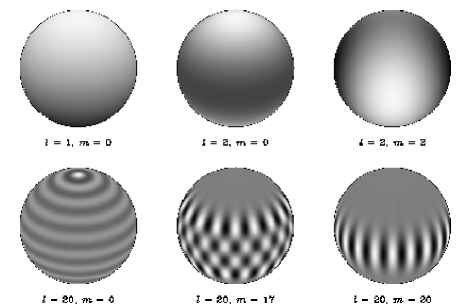
FIG. 2.: Examples of spherical harmonics, labelled by the degree $l$ and azimuthal order $m$. For clarity the polar axis has been inclined $30^{\circ}$ relative to the plane of the page.

A few examples of spherical harmonics are shown in Fig. 2. It should be noticed that with increasing degree the sectoral modes, with $m=\pm l$, become increasingly confined near the equator.

Given the separation of variables, the equations of adiabatic stellar pulsation are reduced to ordinary differential equations for the amplitude functions; writing the equations in terms of the variables $\{\xi_{r},\;p^{\prime},\;\Phi^{\prime},\;{\rm d}\Phi^{\prime}/{\rm d}r\}$ (where I have dropped the tildes) it is straightforward to obtain

$${{\rm d}\xi_{r}\over{\rm d}r}= - \left({2\over r}+{1\over\Gamma_{1}p}{{\rm d}p\over{\rm d}r}\right)\xi_{r}+{1\over\rho c^{2}}\left({S_{l}^{2}\over\omega^{2}}-1\right)p^{\prime}$$ (31)

$$+ {l(l+1)\over\omega^{2}r^{2}}\Phi^{\prime}\;,$$ (32)

$${{\rm d}p^{\prime}\over{\rm d}r}=\rho(\omega^{2}-N^{2})\xi_{r}+{1\over\Gamma_{1}p}{{\rm d}p\over{\rm d}r}p^{\prime}-\rho{{\rm d}\Phi^{\prime}\over{\rm d}r}\;,$$ (33)

and

$${1\over r^{2}}{{\rm d}\over{\rm d}r}\left(r^{2}{{\rm d}\Phi^{\prime}\over{\rm d}r}\right)=4\pi G\left({p^{\prime}\over c^{2}}+{\rho\xi_{r}\over g}N^{2}\right)+{l(l+1)\over r^{2}}\Phi^{\prime}\;.$$ (34)

Here

$$c^{2}={\Gamma_{1}p\over\rho}$$ (35)

is the squared adiabatic sound speed, and I have introduced the characteristic frequencies $S_{l}$ and $N$ (the so-called Lamb and buoyancy frequencies), defined by

$$S_{l}^{2}={l(l+1)c^{2}\over r^{2}}\simeq k_{\rm h}^{2}c^{2}\;,$$ (36)

and

$$N^{2}=g\left({1\over\Gamma_{1}p}{{\rm d}p\over{\rm d}r}-{1\over\rho}{{\rm d}\rho\over{\rm d}r}\right)\;.$$ (37)

The equations must be combined with boundary conditions: two of these ensure regularity at the center, $r=0$, which is a regular singular point of the equations. One condition enforces continuity of $\Phi^{\prime}$ and its gradient at the surface, $r=R$. Finally, the surface pressure perturbation must satisfy a dynamical condition. In its most simple form it imposes zero pressure perturbation on the perturbed surface, i.e.,

$$\delta p=0\qquad{\rm at}\qquad r=R\;.$$ (38)

The fourth-order system of differential equations, Eqs (32) – (34), and the boundary conditions define an eigenvalue problem which has solutions only for selected discrete values of $\omega$. Thus for each $(l,m)$ we obtain a set of eigenfrequencies $\omega_{nlm}$, distinguished by their radial order $n$.

It should be noticed that in the present case of a spherically symmetric star the frequencies are degenerate in azimuthal order: the definition of $m$ is tied to the orientation of the coordinate system which, for a spherically symmetric star, can have no physical significance. Indeed, the equations and boundary conditions do not depend on $m$. Thus, in analyzing the effects of the spherically symmetric structure of the Sun, the frequencies are characterized solely by $l$ and $n$; the relation between structure and these multiplet frequencies $\omega_{nl}$ is discussed in Sections V B – V D. As discussed in Section V E, the degeneracy in $m$ is lifted by rotation.

B Properties of oscillations

From the point of view of helio- and asteroseismic investigations, it is important to realize which aspects of stellar structure are accessible to study, in the sense of having a direct effect on the oscillation frequencies. Within the adiabatic approximation it follows from Eqs (32) – (34) that the frequencies are completely determined by specifying $p$, $\rho$, $g$ and $\Gamma_{1}$ as functions of the distance $r$ to the center. However, assuming that the equations of stellar structure are satisfied, $p$, $g$ and $\rho$ are related by Eqs (3), (4) and (13). Thus specifying just $\rho(r)$ and $\Gamma_{1}(r)$, say, completely determines the adiabatic oscillation frequencies. Conversely, the observed frequencies only provide direct information about these ‘mechanical’ quantities. To constrain other properties of the stellar interior, additional information has to be included, such as the equation of state or Eqs (5) and (6) determining the temperature gradient and luminosity (e.g., Gough and Kosovichev, 1990). It is evident that the inferences obtained in such investigations may suffer from uncertainties in, for example, the assumed physics.

The observed solar oscillations are in most cases predominantly of acoustic nature, and hence there frequencies are most sensitive to sound speed. To interpret helioseismic inferences of sound speed in terms of quantities more directly related to the properties of solar models, it is instructive to note that equation of state of stellar interiors is reasonably well approximated by that of a perfect, fully ionized gas, according to which $p=k_{\rm B}\rho T/(\mu m_{\rm u})$; here $k_{\rm B}$ is Boltzman’s constant, $m_{\rm u}$ is the atomic mass unit, and $\mu$ is the so-called mean molecular weight, related to the abundances $X$ and $Z$ of hydrogen and heavy elements by $\mu\simeq 4/(3+5X-Z)$. In this approximation, also, $\Gamma_{1}=5/3$. Thus

$$c^{2}\simeq{\Gamma_{1}k_{\rm B}T\over\mu m_{\rm u}}\;,$$ (39)

i.e., the sound speed is essentially determined by $T/\mu$. To obtain separate estimates of $T$ and $\mu$, additional constraints on the model are required.

The near-surface layers of the Sun present special problems which have so far not been resolved. Modelling of the structure of these layers is complicated by the presence of convective motions with Mach numbers approaching 0.5, in the uppermost few hundred km of the convection zone. Results of detailed three-dimensional and time-dependent hydrodynamical simulations have been incorporated in a solar model used to compute oscillation frequencies, resulting in some improvement in the agreement with the observed frequencies (Rosenthal et al., 1999); however, in general simple prescriptions, which are certainly inadequate, are used for the treatment of convection in this region. The adiabatic approximation used in most computations of solar oscillation frequencies is not valid near the surface. Even in the cases where nonadiabatic calculations have been carried out (e.g., Guzik and Cox, 1991; Guenther, 1994), these suffer from neglect, or inadequate treatment, of the perturbations to the convective flux; furthermore, the perturbation to the turbulent pressure is usually ignored. These potential problems with the models must be kept in mind when the observed and computed frequencies are compared. However, it is important to note that they are in all cases confined to a very thin region near the solar surface.

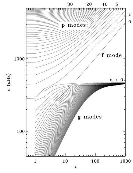
FIG. 3.: Cyclic frequencies $\nu=\omega/2\pi$, as functions of degree $l$, computed for a normal solar model. Selected values of the radial order $n$ have been indicated.

Figure 3 illustrates adiabatic oscillation frequencies computed for a solar model. For clarity modes of given radial order $n$ have been connected. With a few unconfirmed exceptions (see Section VI B 3) the observed solar oscillations have frequencies in excess of 500 $\,\mu{\rm Hz}$ (e.g., Schou, 1998a; Bertello et al., 2000; Finsterle and Fröhlich, 2001; García et al., 2001), and hence correspond to the modes labelled ‘p modes’ and, at relatively high degree ‘f modes’. As discussed in more detail in the following section, the former are standing acoustic waves, whereas the latter behave essentially as surface gravity waves. The modes labelled ‘g modes’ are internal gravity waves. As indicated, it is conventional to assign positive and negative radial orders $n$ to p and g modes, respectively, with $n=0$ for f modes. With this definition, frequency is an increasing function of $n$ for given $l$; also, in most cases $|n|$ corresponds to the number of radial nodes in the radial component of the displacement, excluding a possible node at the center.

In Figure 3 it appears that the f-mode curve crosses the g-mode curves; in fact, if $l$ is regarded as a continuous variable, it is found that the interaction takes place through avoided crossings where the frequencies approach very closely without actually crossing (e.g. Christensen-Dalsgaard 1980). This type of behavior is commonly seen for stellar oscillation frequencies, as a parameter characterizing the solution is varied (e.g. Osaki 1975). It is also well-known in, for example, atomic physics; an early and very clear discussion of the behavior of eigenvalues in the vicinity of an avoided crossing was given by von Neuman & Wigner (1929).

C Asymptotic behavior of stellar oscillations

Although it is relatively straightforward to solve the equations of adiabatic stellar oscillation, approximate techniques play a major role in the interpretation of observations of solar and stellar oscillations. They provide insight into the relation between the observations and the properties of the stellar interiors, which can inspire more precise analyses. Also, since the observed solar modes are in many cases of high order, asymptotic expressions are sufficiently precise to provide useful quantitative results.

1 Properties of acoustic modes

Most of the modes observed in the Sun are essentially acoustic modes, often of relatively high radial order. In this case an asymptotic description can be obtained very simply, by approximating the modes locally by plane sound waves, satisfying the dispersion relation

$$\omega^{2}=c^{2}|{\bf k}|^{2}\;,$$

where ${\bf k}=k_{r}{\bf a}_{r}+{\bf k}_{\rm h}$ is the wave vector. Thus the properties of the modes are entirely controlled by the variation of the adiabatic sound speed $c(r)$. To describe the radial variation of the mode, we use Eq. (29) to obtain

$$k_{r}^{2}={\omega^{2}\over c^{2}}-{L^{2}\over r^{2}}={\omega^{2}\over c^{2}}\left(1-{S_{l}^{2}\over\omega^{2}}\right)\;.$$ (40)

This equation can be interpreted very simply in geometrical terms through the behavior of rays of sound, as illustrated in Fig. 4. With increasing depth beneath the surface of a star temperature, and hence sound speed, increases. As a result, waves that are not propagating vertically are refracted, as indicated in Eq. (40) by the decrease in $k_{r}$ with increasing $c$; the horizontal component $|{\bf k}_{\rm h}|$ of the wave vector, in contrast, increases with decreasing $r$. Thus the rays bend, as shown in Fig. 4. The waves travel horizontally at the lower turning point, $r=r_{\rm t}$, where $\omega=S_{l}$ and hence $k_{r}=0$, i.e.,

$${c(r_{\rm t})\over r_{\rm t}}={\omega\over L}\;.$$ (41)

For $r<r_{\rm t}$, $k_{r}$ is imaginary and the wave decays exponentially.

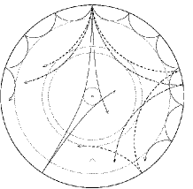
FIG. 4.: Propagation of rays of sound in a cross-section of the solar interior. The ray paths are bent by the increase in sound speed with depth until they reach the inner turning point (indicated by the dotted circles) where they undergo total internal refraction. At the surface the waves are reflected by the rapid decrease in density.

The normal modes observed as global oscillations on the stellar surface arise through interference between waves propagating in this manner. In particular, they share with the waves the total internal reflection at $r=r_{\rm t}$. It follows from Eq. (41) that the lower turning point is located the closer to the center, the lower is the degree or the higher is the frequency. Radial modes, with $l=0$, penetrate the center, whereas the modes of highest degree observed in the Sun, with $l{\leavevmode\kern 3.00003pt\raise 1.29167pt\hbox{$>$}\kern-8.00003pt\lower 3.01385pt\hbox{$\sim$}\kern 3.00003pt}1000$, are trapped in the outer small fraction of a per cent of the solar radius. Thus the oscillation frequencies of different modes reflect very different parts of the Sun; it is largely this variation in sensitivity which allows the detailed inversion for the properties of the solar interior as a function of position (see also Sections VII and VIII).

Equation (40) can be used to justify an approximate, but extremely useful, expression for the frequencies of acoustic oscillation. The requirement of a standing wave in the radial direction implies that the integral of $k_{r}$ over the region of propagation, between $r=r_{\rm t}$ and $R$, must be an integral multiple of $\pi$, apart from possible effects of phase changes at the end-points of the interval:

$$(n+\alpha)\pi\simeq\int_{r_{\rm t}}^{R}k_{r}{\rm d}r\simeq\int_{r_{\rm t}}^{R}{\omega\over c}\left(1-{S_{l}^{2}\over\omega^{2}}\right)^{1/2}{\rm d}r\;,$$ (42)

where $\alpha$ contains the phase changes at the points of reflection. This may also be written as

$${\pi(n+\alpha)\over\omega}\simeq F\left({\omega\over L}\right)\;,$$ (43)

where

$$F(w)=\int_{r_{\rm t}}^{R}\left(1-{c^{2}\over w^{2}r^{2}}\right)^{1/2}{{\rm d}r\over c}\;.$$ (44)

That the observed frequencies of solar oscillation satisfy the simple functional relation given by Eq. (43) was first found by Duvall (1982); this relation is therefore commonly known as the Duvall law.

2 A proper asymptotic treatment

Although instructive, this derivation is hardly satisfactory, in either a mathematical or physical sense. It ignores the fact that the oscillations are not purely acoustic of nature, and neglects effects of variations of stellar structure with position. Also, effects near the stellar surface leading to reflection of the waves are simply postulated.

A more satisfactory description can be based on asymptotic analyses of the oscillation equations, Eqs (32) – (34). The modes observed in the Sun are either of high radial order or high degree. In such cases it is often possible, in approximate analyses, to make the so-called Cowling approximation, where the perturbation $\Phi^{\prime}$ to the gravitational potential is neglected (Cowling, 1941). This can be justified, at least partly, by noting that for modes of high order or high degree, and hence varying rapidly as a function of position, the contributions from regions where $\rho^{\prime}$ have opposite sign largely cancel in $\Phi^{\prime}$. In this approximation, the order of the equations is reduced to two, making them amenable to standard asymptotic techniques (e.g., Ledoux, 1962; Vandakurov, 1967; Smeyers, 1968). A convenient formulation has been derived by Gough (see Deubner and Gough, 1984; Gough, 1993): in terms of the quantity

$$\Psi=c^{2}\rho^{1/2}{\rm div\,}\pmb{{\hbox{\delta}}}{\bf r}\;,$$ (45)

the oscillation equations can be approximated by

$${{\rm d}^{2}\Psi\over{\rm d}r^{2}}=-K(r)\Psi\;,$$ (46)

where

$$K(r)={\omega^{2}\over c^{2}}\left[1-{\omega_{\rm c}^{2}\over\omega^{2}}-{S_{l}^{2}\over\omega^{2}}\left(1-{N^{2}\over\omega^{2}}\right)\right]\;.$$ (47)

Here $N^{2}$ and $S_{l}^{2}$ were defined in Eqs (36) and (37), and the acoustical cut-off frequency $\omega_{\rm c}$ is given by

$$\omega_{\rm c}^{2}={c^{2}\over 4H^{2}}\left(1-2{{\rm d}H\over{\rm d}r}\right)\;,$$ (48)

where $H=-({\rm d}\ln\rho/{\rm d}r)^{-1}$ is the density scale height.

In addition to the modes determined by Eq. (46), there are modes for which ${\rm div\,}\pmb{$\delta$}{\bf r}\simeq 0$; these modes clearly cannot be analyzed in terms of $\Psi$. They approximately correspond to surface gravity waves, with frequencies satisfying

$$\omega^{2}\simeq gk_{\rm h}\;,$$ (49)

and are usually known as f modes. I return to them in Section V C 4.

FIG. 5.: Characteristic frequencies $N/2\pi$ (solid line), $\omega_{\rm c}/2\pi$ (dotted line) and $S_{l}/2\pi$ (dashed lines, labelled by $l$) for $l=1$, 10, 50, 100 and 500. The frequencies have been computed for Model S of Christensen-Dalsgaard et al. (1996). The heavy horizontal lines mark the trapping regions of a g mode of frequency $100\,\mu{\rm Hz}$ and a p mode of frequency $3000\,\mu{\rm Hz}$ and degree $l=10$.

The physical meaning of Eq. (46) becomes clear if we make the identification $K=k_{r}^{2}$ where, as before, $k_{r}$ is the radial component of the local wave number. Accordingly, a mode oscillates as a function of $r$ in regions where $K>0$; such regions are referred to as regions of propagation. The mode is evanescent, decreasing or increasing exponentially, where $K<0$. The detailed behavior of the mode is thus controlled by the value of the frequency, relative to the characteristic frequencies $S_{l}$, $N$ and $\omega_{\rm c}$.

Figure 5 illustrates the characteristic frequencies in a model of the present Sun. It is evident that $\omega_{\rm c}$ is large only near the stellar surface, where the density scale height is small. In the range of observed solar oscillations the frequencies are higher than the buoyancy frequency; thus, roughly speaking, modes have an oscillatory behavior where $\omega>S_{l}$ and $\omega>\omega_{\rm c}$. Another type of propagation occurs at low frequency, in a region where $\omega<N$. Examples of propagation regions corresponding to these two cases are marked in Fig. 5. Modes corresponding to the former case are called p modes; it follows from the analysis given above that they are essentially standing sound waves, where the dominant restoring force is pressure. Modes corresponding to the latter cases are called g modes; here the dominant restoring force is buoyancy, and the modes have the character of standing internal gravity waves.

Equations (46) and (47) are in a form well suited for JWKB analysis. The result is that the modes satisfy

$$\omega\int_{r_{1}}^{r_{2}}\left[1-{\omega_{\rm c}^{2}\over\omega^{2}}-{S_{l}^{2}\over\omega^{2}}\left(1-{N^{2}\over\omega^{2}}\right)\right]^{1/2}{{\rm d}r\over c}\simeq\pi(n-1/2)\;,$$ (50)

where $r_{1}$ and $r_{2}$ are adjacent zeros of $K$ such that $K>0$ between them.

3 Asymptotic properties of p modes

For the p modes, we may approximately neglect the term in $N$ and, except near the surface, the term in $\omega_{\rm c}$. Thus we recover Eq. (40); in particular, the location of the lower turning point is approximately given by Eq. (41). Near the surface, on the other hand, $S_{l}\ll\omega$ for small or moderate $l$ and may be neglected (cf. Fig. 5); thus the location $r=R_{\rm t}$ of the upper turning point is determined by $\omega\simeq\omega_{\rm c}$. Physically, this corresponds to the reflection of the waves where the wavelength becomes comparable to the local density scale height. It should also be noticed from Fig. 5 that $\omega_{\rm c}$ approximately tends to a constant in the stellar atmosphere. Modes with frequencies exceeding the atmospheric value of $\omega_{\rm c}$ are only partially trapped, losing energy in the form of running waves in the solar atmosphere; hence they may be expected to be rather strongly damped.

If we assume that $|N^{2}/\omega^{2}|\ll 1$, Eq. (50) simplifies to

$$\omega\int_{r_{1}}^{r_{2}}\left(1-{\omega_{\rm c}^{2}\over\omega^{2}}-{S_{l}^{2}\over\omega^{2}}\right)^{1/2}{{\rm d}r\over c}\simeq\pi(n-1/2)\;,$$ (51)

where, as discussed above, $r_{1}\simeq r_{\rm t}$ and $r_{2}\simeq R_{\rm t}$. Further simplification results by noting that since $\omega_{\rm c}/\omega\ll 1$, except near the upper turning point, the integral may be expanded, yielding

$$\omega\int_{r_{\rm t}}^{R}\left(1-{S_{l}^{2}\over\omega^{2}}\right)^{1/2}{{\rm d}r\over c}\simeq\pi[n+\alpha(\omega)]\;$$ (52)

(e.g., Christensen-Dalsgaard and Pérez Hernández, 1992). Here we again assumed that $S_{l}\ll\omega$ near the upper turning point; consequently $\alpha$ depends only on frequency and results from the expansion of the near-surface behavior of $\omega_{\rm c}$. Thus we recover Eqs (43) and (44), previously obtained from a simple analysis of sound waves. From a physical point of view, the assumption on $S_{l}$ ensures that the waves travel nearly vertically near the surface; thus their behavior is independent of their horizontal structure, leading to a phase shift depending solely on frequency.

For low-degree modes these relations may be simplified even further, by noting that in the integrand in Eq. (44) $(\ldots)^{1/2}$ differs from unity only close to the lower turning point which, for these modes, is situated very close to the center. As a result it is possible to expand the integral to obtain, to lowest order, that $F(w)\simeq\int_{0}^{R}{\rm d}r/c-w^{-1}\pi/2$. Furthermore, a more careful analysis shows that for low-degree modes $L$ should be replaced by $l+1/2$ (e.g., Vandakurov, 1967; Tassoul, 1980). Thus from Eq. (43) we obtain

$$\nu_{nl}\equiv{\omega_{nl}\over 2\pi}\simeq\left(n+{l\over 2}+{1\over 4}+\alpha\right)\Delta\nu\;,$$ (53)

where $\Delta\nu=[2\int_{0}^{R}{\rm d}r/c]^{-1}$ is the inverse of twice the sound travel time between the center and the surface. This equation predicts a uniform spacing $\Delta\nu$ in $n$ of the frequencies of low-degree modes. Also, modes with the same value of $n+l/2$ should be almost degenerate, $\nu_{nl}\simeq\nu_{n-1\,l+2}$. This frequency pattern was first observed for the solar five-minute modes of low degree by Claverie et al. (1979) and may be used in the search for stellar oscillations of solar type.

The deviations from the simple relation (53) have considerable diagnostic potential. By extending the expansion of Eq. (44), leading to Eq. (53), to take into account the variation of $c$ in the core one finds (Gough, 1986; see also Tassoul, 1980)

$$d_{nl}\equiv\nu_{nl}-\nu_{n-1\,l+2}\simeq-(4l+6){\Delta\nu\over 4\pi^{2}\nu_{nl}}\int_{0}^{R}{{\rm d}c\over{\rm d}r}{{\rm d}r\over r}\;;$$ (54)

here the integral is predominantly weighted towards the center of the star, as a result of the factor $r^{-1}$ in the integrand. This behavior provides an important diagnostic of the structure of stellar cores. In particular, we note that, according to Eq. (39), the core sound speed is reduced as $\mu$ increases with the conversion of hydrogen to helium as the star ages. As a result, $d_{nl}$ is reduced, thus providing a measure of the evolutionary state of the star (e.g., Christensen-Dalsgaard, 1984, 1988; Ulrich, 1986; Gough and Novotny, 1990; see also Gough, 2001a).

It is interesting to investigate the effects on the frequencies of small changes to the model. Such frequency changes may be estimated quite simply by linearizing the Duvall law in differences $\delta\omega_{nl}$ in $\omega_{nl}$, $\delta_{r}c(r)$ in $c(r)$ and $\delta\alpha(\omega)$ in $\alpha(\omega)$. The result can be written (Christensen-Dalsgaard et al., 1988)

$$S_{nl}{{\delta\omega_{nl}}\over{\omega_{nl}}}\simeq{\cal H}_{1}\left({{\omega_{nl}}\over L}\right)+{\cal H}_{2}(\omega_{nl})\;,$$ (55)

where

$$S_{nl}=\int_{r_{\rm t}}^{R}\left(1-{{L^{2}c^{2}}\over{r^{2}\omega_{nl}^{2}}}\right)^{-1/2}{{{\rm d}r}\over c}-\pi{{{\rm d}\alpha}\over{{\rm d}\omega}}\;,$$ (56)

$${\cal H}_{1}({w})=\int_{r_{\rm t}}^{R}\left(1-{{c^{2}}\over{r^{2}{w}^{2}}}\right)^{-1/2}{{\delta_{r}c}\over c}{{{\rm d}r}\over c}\;,$$ (57)

and

$${\cal H}_{2}(\omega)={{\pi}\over{\omega}}\delta\alpha(\omega)\;.$$ (58)

Christensen-Dalsgaard, Gough, and Thompson (1989) noted that ${\cal H}_{1}(\omega/L)$ and ${\cal H}_{2}(\omega)$ can be obtained separately, to within a constant, by means of a double-spline fit of the expression (55) to p-mode frequency differences. The dependence of ${\cal H}_{1}$ on $\omega/L$ is determined by the sound-speed difference throughout the star; in fact, it is straightforward to verify that the contribution from ${\cal H}_{1}$ is essentially just an average of $\delta_{r}c/c$, weighted by the sound-travel time along the rays characterizing the mode. The contribution from ${\cal H}_{2}(\omega)$ depends on differences in the upper layers of the models. Thus, in particular, it contains the effects of the near-surface errors discussed in Section V B.

The preceding, relatively simple, asymptotic analysis has been improved in several investigations. For modes of high degree the expansion leading to a frequency-dependent phase function $\alpha(\omega)$ in Eq. (52) is no longer valid; Brodsky and Vorontsov (1993) showed how the analysis could be generalized to obtain the $l$-dependence of $\alpha$. For modes of low degree or relatively low frequency the perturbation to the gravitational potential can no longer be ignored, and it may furthermore be necessary to include the effect of the buoyancy frequency in the asymptotic dispersion relation (e.g., Vorontsov, 1989, 1991; Gough, 1993). Finally, the usual asymptotic expansion, as used for example to obtain Eq. (54), is somewhat questionable in the core of the star where conditions vary on a scale comparable with the wavelengths of the modes; here other formulations may be more appropriate (e.g., Roxburgh and Vorontsov, 1994a, 2000ab, 2001). However, for the present review the simpler expressions are generally adequate.

4 f and g modes

In addition to p modes, the observations of solar oscillations also show f modes of moderate and high degree. As discussed above, these modes are approximately divergence-free, with frequencies given by (cf. Eq. 49)

$$\omega^{2}\simeq g_{\rm s}k_{\rm h}={GM\over R^{3}}L\;,$$ (59)

where $g_{\rm s}$ is the surface gravity. It may be shown that the displacement eigenfunction is approximately exponential, $\xi_{r}\propto\exp(k_{\rm h}r)$, as is the case for surface gravity waves in deep water. According to Eq. (59) the frequencies of these modes are independent of the internal structure of the star; this allows the modes to be uniquely identified in the observed spectra, regardless of possible model uncertainties. A more careful analysis must take into account the fact that gravity varies through the region over which the mode has substantial amplitude; this results in a weak dependence of the frequencies on the density structure (Gough, 1993).

I finally briefly consider the properties of g modes. It follows from Fig. 5 that these are trapped in the radiative interior and behave exponentially in the convection zone. In fact, they have their largest amplitude close to the solar center and hence are potentially very interesting as probes of conditions in the deep solar interior. High-degree g modes are very effectively trapped by the exponential decay in the convection zone and are therefore unlikely to be visible at the surface. However, for low-degree modes the trapping is relatively inefficient, and hence the modes might be expected to be observable, if they were excited to reasonable amplitudes. The behavior of the oscillation frequencies can be obtained from Eq. (50). In the limit where $\omega\ll N$ in much of the radiative interior this shows that the modes are uniformly spaced in oscillation period, with a period spacing that depends on degree.

D Variational principle

The formulation of the oscillation equations given in Eq. (22) is the starting point for powerful analyses of general properties of stellar pulsations. For convenience, we write the equation as

$$\omega^{2}\pmb{{\hbox{\delta}}}{\bf r}={\cal F}(\pmb{{\hbox{\delta}}}{\bf r})\;,$$ (60)

where the right-hand side is the linearized force per unit mass, which, as discussed in Section V A 2, can be regarded as a linear operator on $\pmb{$\delta$}{\bf r}$.

The central result is that Eq. (60), applied to adiabatic oscillations, defines a variational principle. Specifically, by multiplying the equation by $\rho\pmb{$\delta$}{\bf r}^{*}$ (‘$*$’ denoting the complex conjugate) and integrating over the volume $V$ of the star, we obtain

$$\omega^{2}={\int_{V}\pmb{{\hbox{\delta}}}{\bf r}^{*}\cdot{\cal F}(\pmb{{\hbox{\delta}}}{\bf r})\rho{\rm d}V\over\int_{V}|\pmb{{\hbox{\delta}}}{\bf r}|^{2}\rho{\rm d}V}\;.$$ (61)

We now consider adiabatic oscillations which satisfy the surface boundary condition given by Eq. (38). In this case it may be shown that the right-hand side of Eq. (61) is stationary with respect to small perturbations to the eigenfunction $\pmb{$\delta$}{\bf r}$ (e.g., Chandrasekhar, 1964).

A very important application of this principle concerns the effect on the frequencies of perturbations to the equilibrium model or other aspects of the physics of the oscillations. Such perturbations can in general be expressed as a perturbation $\delta{\cal F}$ to the force in Eq. (60). It follows from the variational principle that their effect on the frequencies can be determined as

$$\delta\omega^{2}={\int_{V}\pmb{{\hbox{\delta}}}{\bf r}^{*}\cdot\delta{\cal F}(\pmb{{\hbox{\delta}}}{\bf r})\rho{\rm d}V\over\int_{V}|\pmb{{\hbox{\delta}}}{\bf r}|^{2}\rho{\rm d}V}\;,$$ (62)

evaluated using the eigenfunction $\pmb{$\delta$}{\bf r}$ of the unperturbed force operator. Applications of this expression to rather general situations were considered by Lynden-Bell and Ostriker (1967).

Equation (62) provides the basis for determining the relation between differences in structure and differences in frequencies between the Sun and solar models. As discussed in Section V B, the oscillation frequencies are determined by a suitable pair of model variables, e.g., the pair $(c^{2},\rho)$, which reflects the acoustic nature of the observed modes. The differences between the structure of the Sun and a model can then be characterized by the differences $\delta_{r}c^{2}/c^{2}=[c_{\odot}^{2}(r)-c_{\rm mod}^{2}(r)]/c^{2}(r)$ and $\delta_{r}\rho/\rho=[\rho_{\odot}(r)-\rho_{\rm mod}(r)]/\rho(r)$. In particular, the perturbation $\delta{\cal F}$ can be expressed in terms of $\delta_{r}c^{2}/c^{2}$ and $\delta_{r}\rho/\rho$, through appropriate use of the linearized versions of Eqs (3) and (4) (e.g., Gough and Thompson, 1991), resulting in a linear relation for the frequency change in terms of the structure differences.

The analysis in terms of $\delta_{r}c^{2}/c^{2}$ and $\delta_{r}\rho/\rho$ only captures the differences between the Sun and the model to the extent that they relate to the hydrostatic structure of the Sun. As discussed in Section V B, inadequacies in the treatment of the physics of the modes, such as nonadiabatic effects, contribute in the near-surface layers of the Sun. These can also be represented as perturbations $\delta{\cal F}_{\rm surf}$, such that $\delta{\cal F}_{\rm surf}(\pmb{$\delta$}{\bf r})$ is significant only in the superficial layers. For modes of low or moderate degree the eigenfunctions depend little on degree in this region, as discussed in Section V C 3. Assuming that $\delta{\cal F}_{\rm surf}$ does not depend explicitly on $l$, it follows that for these modes $\int_{V}\pmb{$\delta$}{\bf r}^{*}\cdot\delta{\cal F}_{\rm surf}(\pmb{$\delta$}{\bf r})\rho{\rm d}V$ depends little on $l$; hence, according to Eq. (62), the effects of the near-surface problems may in general be expected to be of the form

$$\left({\delta\omega_{nl}\over\omega_{nl}}\right)_{\rm surf}\simeq I_{nl}^{-1}F_{\rm surf}(\omega_{nl})\;,$$ (63)

where $I_{nl}=\int_{V}|\pmb{$\delta$}{\bf r}|^{2}\rho{\rm d}V$, the denominator in Eq. (62), is known as the mode inertia and, as indicated, $F_{\rm surf}$ depends only on frequency. We note also that at relatively low frequency the relevant superficial layers are outside the upper turning point determined by $\omega=\omega_{\rm c}$ (cf. Fig. 5) and hence the modes are evanescent in this region. Thus we expect the effects of the near-surface problems to be small for low-frequency modes (e.g., Christensen-Dalsgaard and Thompson, 1997).

The mode inertia still depends on both degree and frequency: in particular, modes of high degree and/or low frequency are trapped closer to the the solar surface (cf. Eq. 41), involve a smaller fraction of the Sun’s mass and hence have a smaller $I_{nl}$. Thus high-degree modes are affected more strongly by the near-surface errors than are low-degree modes at the same frequency. To eliminate this essentially trivial effect, it is instructive to consider frequency differences scaled by $I_{nl}$. This may be done conveniently by scaling the frequencies by

$$Q_{nl}\equiv{I_{nl}\over\bar{I}_{0}(\omega_{nl})}\;,$$ (64)

where $\bar{I}_{0}(\omega_{nl})$ is the inertia of a hypothetical radial mode (with $l=0$) with frequency $\omega_{nl}$, obtained by interpolation to that frequency in the inertias for the actual radial modes. This effectively reduces the frequency shift to the effect on a radial mode of the same frequency. Examples of scaled frequency differences will be shown later.

From the preceding analysis it finally follows that the frequency differences between the Sun and the model, assuming that the differences are so small that a linear representation is adequate, can be written as

$${\delta\omega_{nl}\over\omega_{nl}} = \int_{0}^{R}\left[K_{c^{2},\rho}^{nl}(r){\delta_{r}c^{2}\over c^{2}}(r)+K_{\rho,c^{2}}^{nl}(r){\delta_{r}\rho\over\rho}(r)\right]{\rm d}r$$ (66)

$$+I_{nl}^{-1}F_{\rm surf}(\omega_{nl})\;,$$

where the kernels $K_{c^{2},\rho}^{nl}$ and $K_{\rho,c^{2}}^{nl}$, which result from manipulating $\delta{\cal F}$, are computed from the eigenfunctions of the reference model (e.g., Dziembowski et al., 1990; Däppen et al., 1991; Gough & Thompson, 1991). This relation forms the basis for inversions of the oscillation frequencies to determine solar structure (see Section VII).

The similarity of Eq. (66) to the asymptotic expressions in Eqs (56) – (58) should be noted. In both cases the frequency differences are separated into contributions from the bulk of the Sun (in the asymptotic case characterized solely by the sound-speed difference) and from the near-surface layers, the latter depending essentially only on frequency after appropriate scaling; indeed, it may be shown that $S_{nl}$ and $I_{nl}$ are closely related.

E Effects of rotation

So far, we have considered only oscillations of a spherically symmetric star; in this case, the frequencies are independent of the azimuthal order $m$. Departures from spherical symmetry lift this degeneracy, causing a frequency splitting according to $m$.

The most obvious, and most important, such departure is rotation; early studies of the effect of rotation were presented by Cowling and Newing (1949) and Ledoux (1949, 1951). A simple description can be obtained by first noting that, according to Eqs (24) and (27), the oscillations depend on longitude $\phi$ and time $t$ as $\cos(m\phi-\omega t)$, i.e., as a wave running around the equator. We now consider a star rotating with angular velocity $\Omega$ and a mode of oscillation with frequency $\omega_{0}$ in a frame rotating with the star; the coordinate system is chosen with polar axis along the axis of rotation. Letting $\phi^{\prime}$ denote longitude in this frame, the oscillation therefore behaves as $\cos(m\phi^{\prime}-\omega_{0}t)$. The longitude $\phi$ in an inertial frame is related to $\phi^{\prime}$ by $\phi^{\prime}=\phi-\Omega t$; consequently, the oscillation as observed from the inertial frame depends on $\phi$ and $t$ as

$$\cos(m\phi-m\Omega t-\omega_{0}t)\equiv\cos(m\phi-\omega_{m}t)\;,$$

where $\omega_{m}=\omega_{0}+m\Omega$. Thus the frequencies are split according to $m$, the separation between adjacent values of $m$ being simply the angular velocity; this is obviously just the result of the advection of the wave pattern with rotation.

This simple description contains the dominant physical effect, i.e., advection, of rotation on the observed modes of oscillation, but it suffers from two problems: it assumes solid-body rotation, whereas the Sun rotates differentially; and it neglects the effects, such as the Coriolis force, in the rotating frame. In a complete description in an inertial frame, including terms linear in the angular velocity, Eq. (22) must be replaced by

$$\omega^{2}\pmb{{\hbox{\delta}}}{\bf r}={1\over\rho}\kern-0.18005pt\hbox{$\nabla$}\kern-8.33336pt\kern 0.35995pt\hbox{$\nabla$}\kern-8.33336pt\kern-0.18005pt\raise 0.28pt\hbox{$\nabla$}p^{\prime}-{\bf g}^{\prime}-{\rho^{\prime}\over\rho}{\bf g}+2m\omega\Omega\pmb{{\hbox{\delta}}}{\bf r}-2i\omega\Omega\kern-6.79993pt\Omega\kern-6.79993pt\Omega\times\pmb{{\hbox{\delta}}}{\bf r}\;,$$ (67)

where $\Omega\kern-6.79993pt\Omega\kern-6.79993pt\Omega$ is the rotation vector, of magnitude $\Omega$ and aligned with the rotation axis. The first term resulting from rotation is the contribution from advection, as discussed above, whereas the last term is the Coriolis force.

The terms arising from rotation obviously correspond to a perturbation to the force operator ${\cal F}$ in Eq. (60); from Eq. (62) the effect on the oscillation frequencies can be obtained on the form

$$\omega_{nlm}=\omega_{nl0}+m\int_{0}^{R}\int_{0}^{\pi}K_{nlm}(r,\theta)\Omega(r,\theta)r{\rm d}r{\rm d}\theta\;,$$ (68)

where the kernels $K_{nlm}$ can be calculated from the eigenfunctions for the non-rotating model. The kernels depend only on $m^{2}$, so that the rotational splitting $\omega_{nlm}-\omega_{nl0}$ is an odd function of $m$. Also, the kernels are symmetrical around the equator; as a result, the rotational splitting is only sensitive to the component of $\Omega$ which is similarly symmetrical.

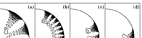
FIG. 6.: Contour plots of rotational kernels $K_{nlm}$ in a solar quadrant. The modes all have frequencies near 2 mHz; the following pairs of $(l,m)$ are included: a) $(5,2)$; b) $(20,8)$; c) $(20,17)$; and d) $(20,20)$.

The general expression for the rotational kernels is quite complicated and will not be given here (see, for example, Hansen et al., 1977; Cuypers, 1980; Gough, 1981). Examples of kernels are shown in Fig. 6. The extent in the radial direction is essentially determined by the location of the lower turning point, $r=r_{\rm t}$ (cf. Eq. 41). The latitudinal extent is determined by the properties of the Legendre functions $P_{l}^{m}$; it follows from their asymptotic behavior that the kernels are confined between latitudes $\pm\cos^{-1}(|m|/L)$. Thus, as also reflected in the behavior of the spherical harmonics (Fig. 2) modes with low $|m|$ extend over essentially all latitudes, whereas modes with $m\simeq\pm l$ are confined close to the equator.

If $\Omega=\Omega(r)$ is assumed to be a function of $r$ alone, the corresponding kernels do not depend on $m$, so that Eq. (68) predicts a uniform frequency splitting in $m$. This is often written on the form

$$\delta\omega_{nlm}\equiv\omega_{nlm}-\omega_{nl0}=m\beta_{nl}\int_{0}^{R}K_{nl}(r)\Omega(r){\rm d}r\;,$$ (69)

where $K_{nl}$ is unimodular, i.e., $\int K_{nl}(r){\rm d}r=1$.

For stars rotating substantially more rapidly than the Sun terms of higher order in $\Omega$ must be taken into account. Terms quadratic in $\Omega$, such as the centrifugal distortion, give rise to frequency perturbations that are even functions of $m$, also changing the mean frequency of the multiplet (e.g., Gough and Thompson, 1990), while cubic terms may be important in cases of modes closely spaced in frequency, such as result from the asymptotic behavior of low-degree p modes (cf. Section V C 3). A detailed discussion of these effects was given by Soufi, Goupil & Dziembowski (1998); they can give rise to complex oscillation spectra, considerably complicating mode identification for rapidly rotating stars.

F The causes of solar oscillations

Given the assumption of adiabatic oscillations, no information is obtained about the possible damping or driving of the modes: the equations are conservative and do not involve any energy exchange between the oscillations and the flow of energy in the equilibrium model. Calculations taking into account nonadiabatic effects have investigated the linear stability of stellar oscillations; this is determined by the imaginary part $\omega_{\rm i}$ of the complex frequency $\omega$, modes with positive $\omega_{\rm i}$ being unstable. It is found that many types of stars, for example the classical Cepheids, have unstable modes; the instability results from favourable phase relations between the compression and the perturbation to the heat flux in the oscillations, often caused by suitable variations in the opacity.

Early nonadiabatic calculations of solar oscillations (e.g., Ando and Osaki, 1975) found that modes in the observed range of frequencies were in fact unstable. These calculations, however, used a simplified treatment of radiative transfer in the outer layers of the Sun and, more importantly, neglected effects of convection. Balmforth (1992a) carried out nonadiabatic calculations of solar oscillations, including convective effects; these were described by expressions, based on mixing-length theory, for the perturbations induced by stellar pulsation to the convective flux and turbulent stresses, developed from an original formulation of Gough (1977a). He found that all the modes were damped, an important contribution to the damping coming from the perturbation to the turbulent pressure.

This motivates a search for driving mechanisms external to the oscillations, the most natural source being the vigorous convection near the solar surface, where motion at near-sonic speed may be expected to be a strong source of acoustic waves (Lighthill, 1952). Stein (1967) applied this to the interpretation of the solar five-minute oscillations. An early estimate of the expected amplitude of global modes excited by this mechanism was made by Goldreich and Keeley (1977).

Since each mode feels the effect of a very large number of turbulent eddies, acting at random, the combined effect is that of a stochastic forcing of the mode. To illustrate the properties of the resulting oscillations I consider a very simple model of this process (Batchelor, 1956; see also Christensen-Dalsgaard, Gough, and Libbrecht, 1989), consisting of a simple damped oscillator of amplitude $A(t)$, forced by a random function $f(t)$, and hence satisfying the equation

$${{\rm d}^{2}A\over{\rm d}t^{2}}+2\eta{{\rm d}A\over{\rm d}t}+\omega_{0}^{2}A=f(t)\;;$$ (70)

here $\eta$ is the linear damping rate, $\eta=-\omega_{\rm i}$. This equation is most easily dealt with in terms of its Fourier transform. Introducing the Fourier transforms $\tilde{A}(\omega)$ and $\tilde{f}(\omega)$ by $\tilde{A}(\omega)=\int A(t)e^{i\omega t}{\rm d}t$, $\tilde{f}(\omega)=\int f(t)e^{i\omega t}{\rm d}t$, we obtain from Eq. (70)

$$-\omega^{2}\tilde{A}-2i\eta\omega\tilde{A}+\omega_{0}^{2}\tilde{A}=\tilde{f}\;.$$ (71)

This yields the power spectrum of the oscillator as

$$P(\omega)=|\tilde{A}(\omega)|^{2}={|\tilde{f}(\omega)|^{2}\over(\omega_{0}^{2}-\omega^{2})^{2}+4\eta^{2}\omega^{2}}\;.$$ (72)

Near the peak in the spectrum, where $|\omega-\omega_{0}|\ll\omega_{0}$ the average power of the oscillation is therefore given by

$$\langle P(\omega)\rangle\simeq{1\over 4\omega_{0}^{2}}{P_{f}(\omega)\over(\omega-\omega_{0})^{2}+\eta^{2}}\;,$$ (73)

where $P_{f}(\omega)=\langle|\tilde{f}(\omega)|^{2}\rangle$ is the average power of the forcing function.

Since $P_{f}(\omega)$ is often a slowly varying function of frequency, the frequency dependence of $\langle P(\omega)\rangle$ is dominated by the denominator in Eq. (73). The resulting profile is therefore approximately Lorentzian, with a width determined by the linear damping rate $\eta$. Consequently, under the assumption of stochastic excitation one can make a meaningful comparison between computed damping rates and observed line widths.

It should be noted that this model makes definite predictions about the oscillation amplitudes, from the power available in the forcing function. This depends on the details of the interaction between convection and the oscillations, with contributions both from Reynolds stresses and entropy fluctuations generated by convection (e.g., Goldreich and Kumar, 1990; Balmforth, 1992b; Goldreich et al., 1994; Samadi et al., 2001; Stein and Nordlund, 2001). The excitation varies strongly with frequency as a result both of the structure of the eigenfunction and the temporal spectrum of convection, hence accounting for the frequency dependence of the mode amplitudes. However, since the horizontal scale of convection near the solar surface is much smaller than the horizontal wavelength of the oscillations, the interaction is likely to depend little on the degree $l$ of the modes; thus, as is indeed observed, we expect excitation of modes at all degrees within the relevant frequency range, with amplitudes that depend relatively little on degree except at high degree (e.g., Christensen-Dalsgaard and Gough, 1982; Woodard et al., 2001).

The observed line profiles show significant departures from the Lorentzian shape, in the form of asymmetries. These can be understood from more complete models of the excitation, taking into account that the dominant contributions to the forcing are spatially localized to relatively thin regions beneath the solar surface (e.g., Duvall et al., 1993a; Gabriel, 1993, 2000; Roxburgh and Vorontsov, 1995; Abrams and Kumar, 1996; Nigam and Kosovichev, 1998; Rast and Bogdan, 1998; Rosenthal, 1998). The observed asymmetry can be used to constrain the depth and other properties of the excitation (Chaplin and Appourchaux, 1999; Kumar and Basu, 1999; Nigam and Kosovichev, 1999) and hence obtain information about subsurface convection.

VI Observation of solar oscillation

Solar oscillations manifest themselves in the solar atmosphere in different ways: the displacement causes the atmosphere to move, changes in the energy transport in the outer layers of the Sun cause oscillations in the solar energy output, while oscillations in the atmospheric temperature are reflected in the properties of the solar spectral lines. Each of these effects may be used to observe the oscillations; since they all reflect the same underlying modes they should evidently yield the same oscillation frequencies. The choice of observing technique is then determined by a combination of technical considerations and noise properties, including the effects of the Earth’s atmosphere for ground-based observations, and effects of other variations in the solar atmosphere. A detailed review of techniques for helioseismic observations and data analysis was given by Brown (1996).

The combined oscillation velocity amplitude in the five-minute range at any given point on the solar surface, as detected by Leighton et al. (1962), is around $500\,{\rm m}\,{\rm s}^{-1}$. However, this results from the random combination of signals from of order $10^{7}$ individual modes. The velocity amplitude for each mode is at most around $10\,{\rm cm}\,{\rm s}^{-1}$. The corresponding amplitude in relative intensity perturbations is a few parts per million. Thus extreme sensitivity is required to carry out detailed observations of the oscillations. Furthermore, the observations have to deal with other fluctuations in the solar atmosphere, such as resulting from near-surface convection and solar activity, of far higher magnitude. That it is even possible to extract the small oscillation signal is in large measure due to the high spatial and temporal coherence of the oscillations, with lifetimes extending over several weeks to months; in contrast, other phenomena in the solar atmosphere typically have low coherence in space and time. Thus, by integrating over the solar disk and analyzing data over extended periods in time, the solar ‘noise’ is suppressed and the oscillations can be isolated; even so, in current observations of solar oscillations the effects of random solar fluctuations are probably the dominant source of background noise. To achieve the noise suppression and the required frequency resolution the observations are typically analyzed coherently over several months; furthermore, temporal gaps in the data introduce frequency sidebands in the power spectrum which complicate the determination of the frequencies, and hence data with minimal interruptions are highly desirable. This immediately points to the need for the combination of data from several sites around the Earth, to compensate for the day/night cycle, or for observations from space.

A Observing techniques

The most detailed observations of solar oscillations have been carried out in line-of-sight velocity, measured from the Doppler shift of lines in the solar spectrum. As illustrated in Fig. 7, this may be done by measuring the intensity in two bands on either side of a suitable spectral line. If the intensities are recorded by means of an imaging detector, the result is a velocity image, measuring simultaneously the motion of the solar surface with potentially high spatial resolution. Alternatively, by passing integrated light from the Sun through the filter to the detector, one obtains a disk-averaged velocity, corresponding to observing the Sun as a star.

The main challenge in the observations is to provide a stable determination of the wavelength intervals defining the two intensities. In an ingenious technique for disk-averaged observations, the filter is replaced by a scattering cell, where light is scattered from the Zeeman-split components of a line in sodium or potassium vapour placed in the field from a permanent magnet (e.g., Fossat and Ricort, 1975; Brookes et al., 1976). Here the wavelength bands are determined mainly by the strength of the field, which is very stable, with little sensitivity to other properties of the instrument. A variant of this technique (e.g., Cacciani and Fofi, 1978) can be used as a magneto-optical transmission filter for spatially resolved observations (e.g., Rhodes et al., 1986; Tomczyk et al., 1995).

The perhaps most extensively developed technique for spatially resolved observation is derived from the so-called Fourier Tachometer (e.g., Brown, 1984). Here the line shift is obtained from four measurements in narrow bands across a given spectral line. This allows the definition of a measure that is essentially linear in the line-of-sight velocity, over the considerable range of velocities encountered over the solar surface. In the actual implementations the spectral bands are defined by Michelson interferometers. Examples of Doppler images obtained using this technique are shown in Fig. 8.

FIG. 7.: Schematic illustration of Doppler-velocity observations. In a), the line-of-sight velocity shifts the line in wavelength by $\Delta\lambda$, from the continuous to the dashed position. This changes the intensities $I_{\rm b}$ and $I_{\rm r}$ measured in the narrow wavelength intervals shown as hatched, as well as the ratio $(I_{\rm b}-I_{\rm r})/(I_{\rm b}+I_{\rm r})$ which provides a measure of the shift and hence of the velocity. Panel b) illustrates the experimental setup. The filter alternates between letting light in the $I_{\rm b}$ and $I_{\rm r}$ bands through. If an imaging detector is used, the resulting images in $I_{\rm b}$ and $I_{\rm r}$ can be combined into a Doppler image.

A conceptually very simple way to study the oscillations is to observe them in broad-band intensity or irradiance. In practice, fluctuations in the Earth’s atmosphere render such observations very difficult from the ground; however, the technique has been highly successful from space (e.g., Woodard and Hudson, 1983; Toutain and Fröhlich, 1992).

A very substantial number of helioseismic observing facilities have been established (see also the review by Duvall, 1995). To limit effects of gaps in the data, networks of observing stations are used. The BiSON (Birmingham Solar Oscillation Network; Chaplin et al., 1996) network was established in 1981 and now consists of six stations; it carries out disk-averaged velocity observations by means of potassium-vapour resonant-scattering cells. Spatially resolved velocity observations are obtained with the GONG (Global Oscillation Network Group; Harvey et al., 1996) six-station network, based on the Fourier-tachometer technique, which has been operational since 1995; this is funded by the US National Science Foundation, but involves a large international collaboration. Valuable data are also being provided by the LOWL instrument of the High Altitude Observatory (Tomczyk et al., 1995) on Mauna Loa, Hawaii, using a magneto-optical filter; this has recently been extended to a two-station network, with the addition of an instrument on Tenerife, in the Canary Islands. Other ground-based networks include the IRIS (Fossat, 1991) and TON (Chou et al., 1995) networks.

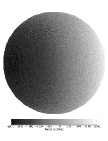
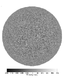
FIG. 8.: Doppler images obtained with the MDI instrument (Scherrer et al., 1995). To the left is the original image, with a greyscale ranging from $-2000\,{\rm m}\,{\rm s}^{-1}$ (dark) to $2000\,{\rm m}\,{\rm s}^{-1}$ (light). This is dominated by solar rotation. After removing rotation by averaging (right-hand image) the mottling associated primarily with solar oscillations becomes apparent; here the greyscale ranges from $-500\,{\rm m}\,{\rm s}^{-1}$ (dark) to $500\,{\rm m}\,{\rm s}^{-1}$ (light).

Space observations from a suitable orbit completely avoid the problem of periodic interruptions of the data. Major contributions have been made from the SOHO spacecraft (Domingo et al., 1995), a joint project between ESA and NASA; it was launched in 1995 and started scientific observations in 1996 from an orbit close to the first Lagrange point between the Earth and the Sun. SOHO carries three helioseismic instruments. GOLF (Global Oscillations at Low Frequency; Gabriel et al., 1995, 1997) aims in particular at detecting low-frequency modes, possibly including g modes, in disk-averaged observations. It was designed as a resonant-scattering Doppler-velocity instrument, using sodium vapour; however technical problems have led to the observations now being carried out in intensity variations in the blue wing of the sodium spectral line. VIRGO (Variability of solar IRradiance and Gravity Oscillations; Fröhlich et al., 1995, 1997) measures solar irradiance, disk-integrated intensities in three different wavelength regions, and intensity with limited spatial resolution. An important goal of the instrument is again the search for g modes, with the hope that these might be more easily detectable in intensity data than in velocity data. Finally, the SOI/MDI (Solar Oscillations Investigation – Michelson Doppler Imager; Scherrer et al., 1995; Rhodes et al., 1997) uses a technique based on the Fourier Tachometer, the spectral bands being defined by a pair of tunable Michelson interferometers. This provides observations of Doppler velocity over the entire solar disk with a spatial resolution of 2 arc sec, corresponding to independent velocity measurements over a total number of about $800\,000$ locations, allowing detailed study of oscillations of degrees up to about 1000.

B Analysis of oscillation data

Regardless of the observing technique, the signal contains contributions from the broad range of modes that are excited in the Sun (cf. Section V F). The goal of the analysis is to extract from this signal, as a function of position on the solar disk and time, information about the properties of the solar interior, such as the structure and internal motions, and about the properties of the excitation of the oscillations. In principle, this may be thought of as fitting to the observations an overall model encompassing all the relevant features. In practice, the analysis must be carried out in several steps, at each step taking into account the properties of the intermediate data resulting from the preceding steps.

Here I concentrate on the determination of the properties of global modes of solar oscillation, most importantly their oscillation frequencies $\omega_{nlm}$, and the subsequent analysis of the frequencies. Alternative analysis techniques, aimed at investigating local properties of the solar interior, are discussed in Section X.

1 Spatial analysis

The first substantial step in the analysis is to separate as far as possible the contributions from the individual spherical harmonics $Y_{l}^{m}$. Oscillations in broad-band or line intensity behave essentially as spherical harmonics as functions of $\theta$ and $\phi$ on the solar disk. For observations in Doppler velocity, the signal is the projection of the velocity field on the line of sight. The surface velocity field for a single mode is determined by Eqs (27) and (28) and is characterized by the ratio $\xi_{\rm h}(R)/\xi_{r}(R)$. It may be shown, however, that at the observed solar frequencies and low or moderate degree the oscillations are predominantly in the radial direction. Thus it is common in the analyses to ignore the horizontal component of velocity.

Here I consider Doppler observations in more detail, assuming the velocity to be purely in the radial direction. For simplicity I furthermore take the axis of the spherical harmonics to be in the plane of the sky, orthogonal to the line of sight. Then the observed Doppler signal $V_{\rm D}$ can be written as

$$V_{\rm D}(\theta,\phi,t) = \sin\theta\cos\phi\sum_{n,l,m}A_{nlm}c_{lm}P_{l}^{m}(\cos\theta)\times$$ (75)

$$\times\cos[m\phi-\omega_{nlm}t-\beta_{nlm}]\;.$$

Here the factor $\sin\theta\cos\phi$ arises from the projection of the velocity onto the line of sight. To isolate modes corresponding to a given spherical harmonic, with $(l,m)=(l_{0},m_{0})$, say, the signal is integrated over the area $A$ of the solar disk, with a suitable weight $W_{l_{0}m_{0}}(\theta,\phi)$, yielding

$$V_{l_{0}m_{0}}(t) = \int_{A}V_{\rm D}(\theta,\phi,t)W_{l_{0}m_{0}}(\theta,\phi){\rm d}A$$ (76)

$$= \sum_{n,l,m}S_{l_{0}m_{0}lm}A_{nlm}\cos[\omega_{nlm}t+\beta_{nlm,l_{0}m_{0}}]\;.$$ (77)

The response function $S_{l_{0}m_{0}lm}$ and the combined phase $\beta_{nlm,l_{0}m_{0}}$ are obtained from integrals of the projected spherical harmonics weighted by $W_{l_{0}m_{0}}$.

The goal of this spatial analysis is obviously to isolate a single spherical harmonic in the time string $V_{l_{0}m_{0}}(t)$, i.e., to have, as far as possible, that $S_{l_{0}m_{0}lm}\propto\delta_{l_{0}l}\delta_{m_{0}m}$, where $\delta_{ij}$ is the Kronecker delta. From the orthogonality of the $Y_{l}^{m}$ over the unit sphere, it may be expected that $W_{l_{0}m_{0}}\simeq Y_{l_{0}}^{m_{0}}$ is suitable. Indeed, had data been available over the entire solar surface, and apart from the velocity projection factor, complete isolation of a single spherical harmonic would have been possible. In practice, however, $V_{l_{0}m_{0}}(t)$ contains contributions also from neighboring $(l,m)$. This so-called leakage substantially complicates the subsequent determination of the oscillation frequencies. Examples of the leakage matrix $S_{l_{0}m_{0}lm}$ are illustrated in Fig. 9.

FIG. 9.: Leakage matrices $S_{l_{0}m_{0}lm}$ for $(l_{0},m_{0})=(10,0)$ (circles) and $(l_{0},m_{0})=(10,10)$ (diamonds), as functions of $(l,m)$. The size of the symbols is proportional to $S_{l_{0}m_{0}lm}$.

A special case of weighting is obtained in disk-averaged observations; in this case the signal is dominated by modes of low degree, $l{\leavevmode\kern 3.00003pt\raise 1.29167pt\hbox{$<$}\kern-8.00003pt\lower 3.01385pt\hbox{$\sim$}\kern 3.00003pt}4$, with no explicit separation between the azimuthal orders (e.g., Dziembowski, 1977; Christensen-Dalsgaard and Gough, 1982). However, since the solar rotation axis is always close to the plane of the sky, it follows from the symmetry of the spherical harmonics that such observations are essentially insensitive to modes where $l-m$ is odd.

In practice, the analysis involves a number of steps. The observed solar Dopplergram is transferred to a co-latitude – longitude grid aligned with the solar rotation axis, taking into account the variation with time of the orientation of the rotation axis relative to the observer. Also, to speed up the calculation of the required very large number of integrals in Eq. (76) the integration in longitude $\phi$ is carried out by means of a Fast Fourier Transform. Some details of these procedures were described by Brown (1985, 1988).

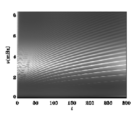
FIG. 10.: Power spectrum of velocity observations from the SOI/MDI experiment on the SOHO spacecraft. The ridges of power concentration correspond to separate radial orders, starting at the lowest frequency with the f mode, with $n=0$.

2 Temporal analysis

The next step in the analysis is to isolate the individual modes, characterized by radial orders $n$, in the time string $V_{l_{0}m_{0}}(t)$. This is done through Fourier analysis of $V_{l_{0}m_{0}}(t)$. The result can be illustrated in a so-called $l-\nu$ diagram, such as is shown in Fig. 10, where the power is plotted against target degree $l_{0}$ and frequency $\nu$. This clearly shows the concentration of power in ridges, each corresponding to a given value of $n$ (cf. Fig. 3). A clearer impression of the power distribution is obtained by plotting the power as a function of frequency, for a given target degree. As a special example, Fig. 11 shows a power spectrum obtained from disk-averaged observations from the BiSON network. It is evident that the power is indeed concentrated in very narrow peaks, hardly resolved at low frequencies; this reflects the intrinsic damping times of the modes which at the lowest frequencies exceed several months. At the maximum power, the amplitude per mode is around $15\,{\rm cm}\,{\rm s}^{-1}$. It should be noticed also that the spectrum reflects the asymptotic frequency behavior for low-degree p modes [cf. Eqs (53) and (54)]: thus several cases of pairs of modes with $l=0,2$ or $l=1,3$ can be identified.

From such spectra, the frequencies and other parameters of the individual modes can be obtained by fitting. This must take into account the statistical nature of the power distribution, resulting from the stochastic excitation (cf. Section V F), and assuming a parametrized form of the average line profile; although in principle asymmetrical profiles should be considered, most analyses to date have been based on Lorentzian profiles characterized by their widths and amplitudes (but see Toutain et al., 1998; Chaplin et al., 1999a; Thiery et al., 2000). The fits are further complicated by the leakage of power from other $(l,m)$ into the spectrum being analyzed.

FIG. 11.: Power spectrum of solar oscillations, obtained from Doppler observations in light integrated over the disk of the Sun. The ordinate is normalized to show velocity power per frequency bin. The data were obtained from six observing stations and span approximately four months. (See Elsworth et al., 1995a.)

To illustrate the quality of present data on solar oscillations, Fig. 12 shows observed mean multiplet frequencies $\nu_{nl}$, obtained from the MDI instrument (Kosovichev et al., 1997). Over a large part of the diagram the errors, even when multiplied by 1000, are barely visible; the relative error $\sigma(\nu)/\nu$ is below $5\times 10^{-6}$ for more than 1000 multiplets. It is this extreme accuracy, in measured quantities related directly to the properties of the solar interior, which allows detailed investigations of solar internal structure.

The ridges in Fig. 12 extend to a limit where the natural line width of the modes is comparable to the separation between modes of adjacent degree; beyond this limit neighboring modes partially merge as a result of the spatial leakage, and a strict separation of modes in frequency becomes difficult or impossible (Howe and Thompson, 1998). At higher degree the mode frequencies must be inferred from the location of ridges containing overlapping contributions from several modes, the relative importance of which depend on the leakage matrix. Thus the frequency determination requires accurate calculation of the leakage matrix, taking also the horizontal component of velocity into account (e.g., Rabello-Soares et al., 2001). Although progress has been made in this area (e.g., Rhodes et al., 2001), more work is required for the determination of fully reliable high-degree frequencies.

FIG. 12.: Observed mean multiplet frequencies of solar oscillations, from 144 days of MDI observations. The error bars correspond to 1000 standard deviations. The smallest relative errors $\sigma(\nu)/\nu$ are below $3\times 10^{-6}$.

The frequency splittings $\Delta\nu_{nlm}=\nu_{nlm}-\nu_{nl}$ contain information about solar internal rotation and other possible departures from spherical symmetry (cf. Section V E). Although full utilization of the information contained in the oscillation data requires use of the individual frequencies $\nu_{nlm}$, the determination of these frequencies is often difficult or impossible. Thus it is customary to represent the frequency splittings by polynomial expansions

$$\nu_{nlm}=\nu_{nl0}+\sum_{j=1}^{j_{\rm max}}a_{j}(n,l)\,{\cal P}_{j}^{(l)}{(m)}\;,$$ (78)

in terms of the so-called $a$ coefficients $a_{j}(n,l)$; here the ${\cal P}_{j}^{(l)}$ are polynomials of degree $j$ which satisfy the orthogonality relation $\sum_{m}{\cal P}_{i}^{(l)}(m){\cal P}_{j}^{(l)}(m)=0$ for $i\neq j$ (e.g., Ritzwoller and Lavely, 1991; Schou et al., 1994). Explicit expressions for these polynomials were given by Pijpers (1997). It follows from Section V E that to lowest order rotation gives rise to odd $a$ coefficients. The even $a$ coefficients correspond to departures from spherical symmetry in solar structure, as well as to quadratic effects of rotation.

3 Solar g modes?

As discussed in Section V C 4, observation of g modes would provide very important information about the properties of the solar core. Indeed, the search for solar g modes has been an important theme in the development of helioseismology. The early indications of a 160-min signal in solar data (cf. Section II) hinted that such modes might be present and led to continued efforts to detect them. An important aspect in these searches was the uniform period spacing that is predicted by asymptotic theory (e.g., Delache and Scherrer, 1983; Fröhlich and Delache, 1984). Unfortunately, although further indications of g modes were presented by Gabriel et al. (1998), the reality of these detections, and the precise nature of the modes, has not yet been definitely established. In particular, Appourchaux et al. (2000a), analyzing several different data sets, obtained stringent upper limits to the amplitudes of solar g modes, substantially lower than the early claims and barely consistent with the results of Gabriel et al. (1998).

C Helioseismic inversion

Given the observed frequencies, an important goal is to infer localized properties about the solar interior from them through inversion. Several inversion techniques have been developed for this purpose. Here I first illustrate general principles by considering the somewhat idealized case of inference of a spherically symmetric angular velocity $\Omega(r)$ from observed rotational splittings (cf. Eq. 69), and then discuss the techniques that are applied in more realistic cases.

1 Principles of inversion

In the simple rotational inversion problem the data are of the form

$$\Delta_{i}=\int_{0}^{R}K_{i}(r)\Omega(r){\rm d}r+\epsilon_{i}\;,\qquad i=1,\ldots,M\;,$$ (79)

where, for notational simplicity, I represent the pair $(n,l)$ by the single index $i$; $M$ is the number of modes in the data set considered, $\Delta_{i}$ is the scaled rotational splitting $m^{-1}\beta_{nl}^{-1}\delta\omega_{nlm}$, and $\epsilon_{i}$ is the observational error in $\Delta_{i}$. The goal of the inversion is to determine an approximation $\bar{\Omega}(r_{0})$ to the true angular velocity, as a function of position $r_{0}$ in the Sun. Inversion is often carried out through linear operations on the data. Hence for each $r_{0}$ there exists a set of inversion coefficients $c_{i}(r_{0})$ such that

$$\bar{\Omega}(r_{0})=\sum_{i}c_{i}(r_{0})\Delta_{i}=\int_{0}^{R}{\cal K}(r_{0},r)\Omega(r){\rm d}r\;,$$ (80)

using Eq. (79) and ignoring the error; here the averaging kernel ${\cal K}(r_{0},r)$ is given by

$${\cal K}(r_{0},r)=\sum_{i}c_{i}(r_{0})K_{i}(r)\;.$$ (81)

The inversion coefficients and averaging kernels clearly depend on the choice of inversion method, and of possible parameters that enter into the method; indeed, the inversion may be thought of as a way to determine coefficients and averaging kernels such as to obtain as much information about the angular velocity as possible.

The averaging kernels provide an indication of the resolution of the inversion; it is clearly desirable to achieve averaging kernels that are sharply peaked around $r=r_{0}$, and with small amplitude far away from that point. The inversion coefficients give information about the propagation of errors from the data to the solution $\bar{\Omega}(r_{0})$. In particular, if the errors $\epsilon_{i}$ are assumed to be uncorrelated, with standard errors $\sigma(\Delta_{i})$, the standard error in the result of the inversion satisfies

$$\sigma[\bar{\Omega}(r_{0})]^{2}=\sum_{i}c_{i}(r_{0})^{2}\sigma(\Delta_{i})^{2}\;.$$ (82)

The optimization of the inversion techniques requires a trade-off between width of the averaging kernels and the error.

In the techniques of optimally localized averages, developed by Backus and Gilbert (1970), the coefficients $c_{i}(r_{0})$ are chosen such as to make ${\cal K}(r_{0},r)$ approximate as far as possible a delta function $\delta(r-r_{0})$ centered on $r_{0}$; then $\bar{\Omega}(r_{0})$ provides an approximation to $\Omega(r_{0})$. In one version this is achieved by determining the coefficients $c_{i}(r_{0})$ such as to minimize

$$\int_{0}^{R}{\cal J}(r_{0},r){\cal K}(r_{0},r)^{2}{\rm d}r+\mu\sum_{i}c_{i}(r_{0})^{2}\sigma(\Delta_{i})^{2}\;,$$ (83)

subject to the constraint

$$\int_{0}^{R}{\cal K}(r_{0},r){\rm d}r=1\;.$$ (84)

Here ${\cal J}(r_{0},r)$ is a weight function which is small close to $r=r_{0}$ and large elsewhere; a common choice is ${\cal J}(r_{0},r)=(r-r_{0})^{2}$. Furthermore, $\mu$ is a parameter which, as discussed below, must be adjusted to optimize the result.

Minimizing the first term in the expression (83) subject to Eq. (84) ensures that ${\cal K}(r_{0},r)$ is large close to $r_{0}$, where the weight function ${\cal J}(r_{0},r)$ is small, and small elsewhere. This is precisely the required “delta-ness” of the combined kernel. The effect of the second term in Eq. (83) is to restrict $\sigma^{2}(\bar{\Omega})$. The size of $\mu$ determines the relative importance of the localization and the size of the variance in the result. Hence, $\mu$ must be determined to ensure a trade-off between the localization and the error, measured by the width of ${\cal K}(r_{0},r)$ and $\sigma[\bar{\Omega}(r_{0})]$, respectively.

Pijpers and Thompson (1992, 1994) developed a computationally more efficient method, where the inversion coefficients are determined by matching ${\cal K}(r_{0},r)$ to a prescribed target function ${\cal T}(r_{0},r)$. They dubbed this the SOLA technique (for Subtractive Optimally Localized Averaging), to distinguish it from the MOLA technique (for Multiplicative Optimally Localized Averaging) discussed above. Specifically, the coefficients $c_{i}(r_{0})$ are determined by minimizing

$$\int_{0}^{R}\left[{\cal K}(r_{0},r)-{\cal T}(r_{0},r)\right]^{2}{\rm d}r+\mu\sum_{i}c_{i}(r_{0})^{2}\sigma(\Delta_{i})^{2}\;,$$ (85)

where again $\mu$ is a trade-off parameter. In addition, the width of ${\cal T}(r_{0},r)$ functions as a parameter, in most cases depending on $r_{0}$, of the method. As before, the inclusion of the last term in Eq. (85) serves to limit the error in the solution. An important advantage of the technique is the ability to choose the target function such as to tailor the averaging kernels to have specific properties.

A second commonly used class of techniques are the regularized least-squares, or Tikhonov, methods (see, for example, Craig and Brown, 1986). Here the solution $\bar{\Omega}(r)$ is parameterized, for example as a piecewise constant function on a grid $r_{0}<r_{1}<\ldots<r_{N}$, with $\bar{\Omega}(r)=\Omega_{j}$ on the interval $[r_{j-1},r_{j}]$; the parameters $\Omega_{j}$ are determined through a least-squares fit to the data. In general, this procedure is regularized to obtain a smooth solution, by including in the minimization a term which restricts the square of $\bar{\Omega}$, or the square of its first or second derivative. Thus, for example one may minimize

$$\sum_{i}\sigma(\Delta_{i})^{-2}\left[\int_{0}^{R}K_{i}(r)\bar{\Omega}(r){\rm d}r-\Delta_{i}\right]^{2}$$ (86)

$$+\mu^{2}\int_{0}^{R}\left({{\rm d}^{2}\bar{\Omega}\over{\rm d}r^{2}}\right)^{2}{\rm d}r\;,$$ (87)

where in the last term a suitable discretized approximation to ${\rm d}^{2}\bar{\Omega}/{\rm d}r^{2}$, in terms of the $\Omega_{j}$, is used. The minimization of Eq. (87) clearly leads to a set of linear equations for $\bar{\Omega}_{j}$, defining the solution; however, it is still the case that the solution is linearly related to the data and hence is characterized by inversion coefficients and averaging kernels (cf. Eq. 80). By restricting the second derivative the last term in Eq. (87) suppresses rapid oscillations in the solution, and hence ensures that it is smooth; the weight $\mu^{2}$ given to this term serves as a trade-off parameter, determining the balance between resolution and error for this method.

Christensen-Dalsgaard et al. (1990) made a comparison of different inversion techniques as applied to this problem, in terms of their error and resolution properties. Useful insight into the properties of inversion techniques can be obtained from analyzing the inverse problem by means of (Generalized) Singular Value Decomposition (e.g., Hansen, 1990, 1994; Christensen-Dalsgaard et al., 1993). This can also be used to develop efficient algorithms for the inversion, through pre-processing of the problem (Christensen-Dalsgaard and Thompson, 1993; Basu et al., 1997a).

It is evidently important to consider the statistical properties of the inferences obtained through helioseismic inversion. This requires reliable information about the statistics of the data (oscillation frequencies or frequency splittings), which may not always be available. An important example is correlation between data errors; although the correlation matrix has been estimated in a few cases (e.g., Schou et al., 1995), off-diagonal elements are generally not taken into account in the inversion. Yet it was demonstrated by Gough (1996a) and Gough and Sekii (2002) that this might have serious effects on the inferences. Howe and Thompson (1996) noted the importance of taking into account also the error correlation between different points in the inference. Careful evaluations of statistical aspects of helioseismic inversion were provided by Genovese et al. (1995) and Gough et al. (1996a).

2 Inversion for solar rotation

In reality, we wish to infer the solar internal angular velocity $\Omega(r,\theta)$ as a function of both distance $r$ to the center and co-latitude $\theta$. Inversions to do so can be based directly on Eq. (68), although quite often the expansion of the rotational splittings in $a$ coefficients (cf. Eq. 78) is used; it is straightforward to show that the odd $a$ coefficients are related to $\Omega(r,\theta)$ by relations similar to Eq. (68), with kernels that may be determined from the kernels $K_{nlm}(r,\theta)$. The inversion methods discussed above can be immediately generalized to the two-dimensional case of inferring functions of $(r,\theta)$, including the definitions of inversion coefficients and averaging kernels (e.g., Schou et al., 1994). The main difficulty, compared to the one-dimensional case, is the amount of data that must be dealt with; while inversion for solar structure, based on average multiplet frequencies, requires the analysis of typically at most a few thousand frequencies, the splittings or $a$ coefficients used for rotational inversion number tens of thousands. For this reason early investigations were typically carried out with the so-called 1.5-dimensional methods (e.g., Brown et al., 1989) where $\Omega(r,\theta)$ was expanded suitably in $\theta$, reducing the problem to a series of one-dimensional inversions for the expansion coefficients as functions of $r$. However, with the development of computer power, and even more with the development of efficient algorithms taking advantage of the detailed structure of the problem (e.g., Larsen, 1997; Larsen and Hansen, 1997), the fully two-dimensional inversions are entirely feasible and commonly used. An overview of inversion methods and further references were given by Schou et al. (1998), who also carried out tests of the inversion procedures based on artificial data.

3 Inversion for solar structure

Inversion for solar structure is conceptually more complicated than the rotational inversion. In the case of rotation, the basic relation between the unknown angular velocity and the data is linear to a high approximation. In the structure case, on the other hand, the corresponding relation between structure and multiplet frequencies is highly nonlinear. This is dealt with through linearization, on the assumption that a solar model is available which is sufficiently close to the actual solar structure; then the inversion can be based on Eq. (66). This is of a form similar to the simple inverse problem in Eq. (79), although with additional terms, and can be analyzed using extensions of the methods discussed in Section VI C 1.

Least-squares inversion can be carried out by parametrizing the unknown functions $\delta_{r}c^{2}/c^{2}$, $\delta_{r}\rho/\rho$ and $F_{\rm surf}$, the parameters being determined through regularized least-squares fitting similar to Eq. (87) (e.g., Dziembowski et al., 1990; Antia and Basu, 1994a); as shown by Basu and Thompson (1996) this allows tests for possible systematic errors in the data through investigation of the residuals. However, most inversions for solar structure differences have applied generalizations of the optimally-localized average techniques, by constructing linear combinations of the relations (66) with coefficient $c_{i}(r_{0})$ chosen to isolate a specific feature of the structure. To infer $\delta_{r}c^{2}/c^{2}$, for example, this is achieved with the SOLA method by replacing the expression (85) to be minimized by

$$\int_{0}^{R}\left[{\cal K}_{c^{2},\rho}(r_{0},r)-{\cal T}(r_{0},r)\right]^{2}{\rm d}r+\beta\int_{0}^{R}{\cal C}_{\rho,c^{2}}(r_{0},r)^{2}{\rm d}r$$ (88)

$$+\mu\sum_{i}\sigma_{i}c_{i}(r_{0})c_{j}(r_{0})\;,$$ (89)

where again $i$ numbers the multiplets $(n,l)$, and $\sigma_{i}$ is the standard error of $\delta\omega_{i}/\omega_{i}$. Here the averaging kernel is now

$${\cal K}_{c^{2},\rho}(r_{0},r)=\sum_{i}c_{i}(r_{0})K_{c^{2},\rho}^{i}(r)$$ (90)

and I have introduced the cross-term kernel

$${\cal C}_{\rho,c^{2}}(r_{0},r)=\sum_{i}c_{i}(r_{0})K_{\rho,c^{2}}^{i}(r)\;,$$ (91)

which controls the (undesired) contribution of $\delta_{r}\rho/\rho$ to the solution. As in the rotation case, the minimization of the expression (89) ensures that ${\cal K}_{c^{2},\rho}(r_{0},r)$ approximates the target ${\cal T}(r_{0},r)$ while suppressing the contributions from the cross term and the data errors; the effect of the term in $F_{\rm surf}$ is reduced by chosing the coefficients to satisfy in addition the constraints

$$\sum_{i}c_{i}(r_{0})I_{i}^{-1}\psi_{\lambda}(\omega_{i})=0\;,\lambda=0,\ldots,\Lambda\;,$$ (92)

for a suitably chosen set of functions $\psi_{\lambda}$, typically taken to be polynomials of order $\lambda$ (e.g., Däppen et al., 1991; Kosovichev et al., 1992). A detailed discussion of implementation details, including the choice of the trade-off parameters $\beta$ and $\mu$ and of the properties of the target function, was provided by Rabello-Soares et al. (1999).

For high-degree modes the surface effects are no longer functions of frequency alone, as demonstrated by Brodsky & Vorontsov (1993). Di Mauro et al. (2002) have developed a generalization of the constraints (92), based on the asymptotic expressions of Brodsky & Vorontsov, allowing suppression of the surface term for modes of degree as high as 1000. The resulting inversion enabled resolution of the upper few per cent of the solar radius, including the helium and parts of the hydrogen ionization zones, of great interest in connection with investigation of the equation of state of the solar plasma (see also Section VII B).

VII Helioseismic investigation of solar structure

The average multiplet frequencies $\nu_{nl}$ carry information about the spherically symmetric component of solar structure. This can be used to test solar models and obtain information about the properties of matter in the solar interior. As noted in Section V B only quantities such as density $\rho$, adiabatic exponent $\Gamma_{1}$ or sound speed $c$ are immediately constrained by the frequencies; constraints on other aspects of the solar interior structure require further assumptions about the models.

Already the early observations of high-degree modes (Deubner, 1975; Rhodes et al., 1977) provided significant constraints on the solar interior. Although these modes are trapped in the outer part of the convection zone, they are sensitive to its general adiabatic structure, and comparison between the observed and computed frequencies indicated that the convection zone was deeper than previously assumed (Gough, 1977b; Ulrich and Rhodes, 1977). Furthermore, it was pointed out that the frequencies were sensitive to details of the equation of state (e.g., Berthomieu et al., 1980; Lubow et al., 1980). The detection of low-degree modes, penetrating to the solar core, allowed tests of more profound aspects of the models, including effects of changes aimed at reducing the neutrino flux (cf. Section IV B). An early result was the likely exclusion of solar models with abundances of helium and heavier elements substantially below the standard values (Christensen-Dalsgaard and Gough, 1980b). Elsworth et al. (1990) obtained strong evidence against non-standard models involving either mixing or energy transport by weakly interacting massive particles. More generally, it is now clear that all models that have been proposed to reduce the solar neutrino flux to the observed values through modifications to solar structure are inconsistent with the helioseismic data.

The determination of frequencies for a broad range degrees by Duvall and Harvey (1983) opened up the possibility for inversions to determine the structure of substantial parts of the solar interior. Gough (1984a) noted that Eq. (44) for the function $F(w)$, determined from observed quantities by Eq. (43), could be inverted, without any reference to a solar model, to determine the sound speed $c$ as a function of $r$. This was applied to solar data by Christensen-Dalsgaard et al. (1985) to infer the sound speed in much of the solar interior, testing the method by applying it to frequencies of solar models. The results showed clear indications of the base of the convection zone, as a change in curvature in $c(r)$; the discrepancies in the radiative interior between the Sun and the model could be interpreted as a deficit in the opacity in the model, as was subsequently confirmed by the opacity calculations by, for example, Iglesias et al. (1992).

Equations (43) and (44) were derived from a very simple form of the asymptotic analysis, and hence the resulting inversion suffers from systematic errors. These can be substantially reduced by basing the inverse analysis on higher-order or otherwise improved asymptotic descriptions (e.g., Vorontsov and Shibahashi, 1991; Marchenkov et al., 2000), maintaining the advantage of being independent of a solar model. Alternatively, the systematic errors can to some extent be eliminated by carrying out a differential asymptotic inversion, based on a fit of Eq. (55) to frequency differences between the Sun and a model (Christensen-Dalsgaard, Gough, and Thompson, 1989); given the resulting ${\cal H}_{1}(w)$, Eq. (57) may be inverted analytically to infer the sound-speed difference between the Sun and the model. This technique was used by Christensen-Dalsgaard et al. (1991) to determine the depth of the solar convection zone as $d_{\rm cz}=(0.287\pm 0.003)R$, a result also obtained independently by Kosovichev and Fedorova (1991); the inference has later been confirmed and substantially tightened by Basu and Antia (1997) and Basu (1998) from fits of ${\cal H}_{1}(w)$ to sequences of models. Using the differential asymptotic technique, Christensen-Dalsgaard, Proffitt, and Thompson (1993) demonstrated that the inclusion of helium settling very substantially reduced the sound-speed differences between solar models and the Sun.

A Inferences of sound speed and density

I now consider in more details the results of inferring solar internal structure from the oscillation frequencies. In much of the discussion I use as reference Model S of Christensen-Dalsgaard et al. (1996); this falls within the category of ‘standard solar models’ (see Section IV A) and has been used quite extensively in helioseismic investigations.

The simplest way to test a solar model is to consider differences between observed frequencies and those of the model. In Fig. 13, panel (a) shows relative differences between observed frequencies presented by Basu et al. (1997b) and those of Model S. Although there is some scatter, the differences depend predominantly on frequency, and furthermore they are quite small at low frequency. According to Section V D this suggests that the dominant contributions to the differences are located in the near-surface layers of the model. This is confirmed by considering differences scaled by $Q_{nl}$ (panel b), where most of the scatter has been suppressed. Indeed, giving the simplifications involved in the modeling of the near-surface structure, and the use of adiabatic frequencies, it is hardly surprising that differences of this magnitude are obtained.

FIG. 13.: (a) Relative frequency differences, in the sense (observation) – (model). The observations are a combination of BiSON whole-disk measurements (e.g., Elsworth et al., 1994) and LOWL observations (Tomczyk et al., 1995), as described by Basu et al. (1997b), while the computed frequencies are for Model S. (b) The same, but scaled by the inertia ratio $Q_{nl}$ (see Section V D). (c) Scaled differences after subtraction of the fitted ${\cal H}_{2}(\nu)$, plotted against $\nu_{nl}/(l+1/2)$ which determines the lower turning point $r_{\rm t}$, shown as the upper abscissa.

Even after scaling, there remains some scatter in the differences, suggesting a dependence on the depth of penetration of the mode and hence the presence of differences between the structure of the Sun and the model that are not confined to the near-surface layers. These effects can be isolated by subtracting a function of frequency fitted to the points in Fig. 13b. The residual (see Fig. 13c) is clearly highly systematic; the small intrinsic scatter reflects both the extremely small observational error and the extent to which frequency differences can be represented by Eq. (55). It is evident that the behavior changes drastically for modes penetrating just beneath the base of the convection zone, with $r_{\rm t}/R{\leavevmode\kern 3.00003pt\raise 1.29167pt\hbox{$<$}\kern-8.00003pt\lower 3.01385pt\hbox{$\sim$}\kern 3.00003pt}0.7$; this suggests that there may be substantial differences between the Sun and the model in this region.

Inversion for the differences in structure, without making asymptotic approximations, was discussed in Section VI C 3. Typical results of such inversions, using the SOLA method, are shown in Fig. 14. To illustrate the resolution properties of the inversion, panel (c) shows selected averaging kernels. It is evident that the inversion has indeed succeeded in resolving the sound-speed difference between the Sun and the model in considerable detail. Also, the 1-$\sigma$ formal errors in the results are extremely small, below $2\times 10^{-4}$ in the bulk of the model, owing to the precision of the observed multiplet frequencies. Other, similar results were obtained by, for example, Gough et al. (1996b) and Kosovichev et al. (1997).

FIG. 14.: Results of sound-speed inversion. (a) Difference in squared sound speed, in the sense (Sun) – (model), inferred from inversion of the differences between the observed BiSON and LOWL frequencies and the frequencies of two solar models: closed circles are for Model S, and open circles for a similar model, but ignoring element diffusion and settling. (b) Results for Model S, on an expanded scale. The vertical error bars are 1-$\sigma$ errors on the inferred differences, while the horizontal bars provide a measure of the resolution of the inversion. (c) Selected averaging kernels ${\cal K}(r_{0},r)$, for fractional target radii $r_{0}/R=0.1,0.3,0.5,0.7,0.8$ and $0.9$. (Adapted from Basu et al., 1997b.)

The inferred difference between the solar and the Model S sound speed (cf. Fig. 14b) is striking. First of all, the overall magnitude should be noted: the difference is everywhere below about $5\times 10^{-3}$, indicating that $c^{2}$ of the model agrees with that of the Sun to within 0.5 per cent from below $0.1R$ to very near the surface. It is important to recall that the model calculation contains no free parameters which have been adjusted to achieve this level of agreement. It is true that the computation of solar models has been improved as a result of the constraints imposed by the steadily improving helioseismic data, through the inclusion of settling as well as through improved equation of state and opacities; as an example, Fig. 14a compares inversion relative to Model S with the use of a corresponding model which does not include diffusion and settling. In this sense the current models have been developed as a result of the helioseismic data. However, the improvements in physics have not been tailored towards fitting the data; it is remarkable that they have nonetheless resulted in a fit as good as the one shown in Fig. 14b.

It should noticed, however, that the differences, although small, are highly significant. Particularly prominent is the peak in $\delta_{r}c^{2}/c^{2}$ just below the convection zone. This is a feature shared by all recent investigations, based on a variety of data and ‘standard’ solar model calculations; interestingly, recent updates to the opacities and the solar initial composition have tended to increase the discrepancies between the Sun and standard solar models. Similarly, the negative $\delta_{r}c^{2}/c^{2}$ around $r=0.2R$ is a common feature to most inferences. On the other hand, the results in the inner core, for $r{\leavevmode\kern 3.00003pt\raise 1.29167pt\hbox{$<$}\kern-8.00003pt\lower 3.01385pt\hbox{$\sim$}\kern 3.00003pt}0.1R$, show some variation between different data sets, although the inferred differences are in all cases of a magnitude similar to that shown in Fig. 14b. The inferences certainly show that standard calculations are inadequate. I return to possible causes for the discrepancies in Section XI.

Extensive comparisons have been carried out between solar models and the results of helioseismic inversions, to investigate effects of changes in the physics of the solar interior. Basu et al. (2000) showed that the inferred solar structure depends little on the assumed reference model, thus confirming that the linearization in Eq. (66) is justified. A detailed analysis of the sensitivity of the helioseismic results to the composition profile and aspects of the nuclear energy generation was presented by Turck-Chièze et al. (2001b).

Although the most general information about the solar interior is obtained from inverse analyses, as discussed above, other techniques may be more sensitive to specific features of the solar interior. In particular, localized features in the Sun cause oscillatory perturbations in the frequencies, as a function of mode order, resulting from the change in the phase of the eigenfunctions at the location of the feature as the order is varied (e.g., Gough, 1990). An interesting example is the rapid change in the temperature gradient at the base of the convection zone, which has a distinct signature in the oscillation frequencies. Analyses of the observed frequencies have been used to show that convective penetration into the radiative region below the convection zone, at least assuming a relatively simple model of the resulting structure, has at most a very limited extent (e.g., Basu et al., 1994; Monteiro et al., 1994; Roxburgh and Vorontsov, 1994b).

B Physics and composition of the solar interior

The precision of the observed frequencies allows us to go beyond the determination of the sound speed, to investigate finer details of the physics of the solar interior. An important aspect is the equation of state, particularly in the regions of partial ionization which to a large extent are found in the convection zone. This part of the Sun has substantial advantages for helioseismic investigations: since the stratification is very nearly adiabatic, apart from a thin region near the top, the structure of the convection zone depends essentially only on the equation of state and composition, while it is not directly affected by the opacity. The potential for helioseismic determination of the convection-zone composition and tests of the equation of state was recognized by Gough (1984b) (see also Däppen and Gough, 1986). An important and potentially detectable effect of the thermodynamic state and composition arises from $\Gamma_{1}$ which is suppressed relative to the value of $5/3$ for a fully ionized ideal gas in the zones of partial ionization of abundant elements (e.g., Däppen, 1998). In particular, determination of the helium abundance is in principle possible because the reduction in $\Gamma_{1}$ in the second ionization zone of helium obviously depends on the abundance of helium.

Investigations of these ionization zones can be carried out in terms of the asymptotic description of the oscillations in Eqs (52) or (55), where the effects of the near-surface regions are contained in the phase functions $\alpha(\omega)$ or ${\cal H}_{2}(\omega)$. As discussed above, the relatively sharp variation of $\Gamma_{1}$ in the second helium ionization zone causes an oscillation in the frequencies, reflected in the phase functions, of a magnitude that depends on the helium abundance. Determinations of the solar envelope helium abundance by means of such asymptotic methods were carried out by Vorontsov et al. (1991), Antia and Basu (1994b), and Pérez Hernández and Christensen-Dalsgaard (1994). Furthermore, the phase functions may provide powerful diagnostics of the equation of state in the near-surface region (e.g., Vorontsov et al., 1992; Baturin et al., 2000).

To discuss the potential of helioseismology for testing composition and thermodynamic properties, beyond the asymptotic approximation, we note that the sound speed is determined by $p$, $\rho$ and $\Gamma_{1}$ (cf. Eq. 35), where, in turn, $\Gamma_{1}=\Gamma_{1}(p,\rho,Y,Z)$ may be obtained from the thermodynamical properties of the gas and the composition; allowance should be made, however, for a possible error $(\delta\Gamma_{1})_{\rm int}$ in the equation of state used in the calculation of the reference model, where $(\delta\Gamma_{1})_{\rm int}$ is the difference in $\Gamma_{1}$ between the values obtained with the solar and the model equations of state, at fixed $p,\rho,Y,Z$. Then Eq. (66) can be rewritten, expressing $\delta_{r}c^{2}$ in terms of $\delta_{r}p$, $\delta_{r}\rho$, $\delta_{r}Y$ and $(\delta\Gamma_{1})_{\rm int}$; it is convenient to express the result in terms of $u=p/\rho$, using also Eqs (3) and (4), to obtain

$${\delta\nu_{nl}\over\nu_{nl}} = \int K^{nl}_{u,Y}{\delta_{r}u\over u}{\rm d}r+\int K^{nl}_{Y,u}\delta_{r}Y{\rm d}r$$ (94)

$$+\int K^{nl}_{c^{2},\rho}\left({\delta\Gamma_{1}\over\Gamma_{1}}\right)_{\rm int}{\rm d}r+{F_{\rm surf}(\nu_{nl})\over I_{nl}}$$

(see also Basu and Christensen-Dalsgaard, 1997). If it is assumed that the model equation of state is adequate, such that $(\delta\Gamma_{1}/\Gamma_{1})_{\rm int}$ is negligible, Eq. (94) may be inverted to determine $\delta_{r}Y$ in the helium ionization zones (e.g., Kosovichev et al., 1992); since the convection zone is fully mixed, this provides a measure of the convection-zone value $Y_{\rm e}$ of the helium abundance. In a regularized least-squares inversion, for example, $\delta_{r}Y$ may be assumed to be constant and hence taken outside the integral in equation Eq. (94) as a single parameter (e.g., Dziembowski et al., 1990, 1991).

In general, potential errors in the equation of state must be taken into account. Basu and Christensen-Dalsgaard (1997) showed how the differences in equation of state might be taken explicitly into account in the inversion, albeit at the expense of an increase in the error in the solution; they also pointed out that the inversion might be carried out to determine the intrinsic difference in $\Gamma_{1}$ between the solar and model equations of state.

To illustrate the sensitivity of such investigations, Fig. 15 shows the results of inversions for $\Gamma_{1}$ in the entire solar interior (Elliot and Kosovichev, 1998). The most striking aspect are the differences in the solar core which are clearly resolved. These demonstrate that the inference is sensitive to the relativistic effects in the treatment of the electrons, which were neglected in the original MHD equation of state used in the top panel, but included in the corrected version used in the bottom panel. Although this is a fairly trivial correction, it does illustrate the sensitivity of the helioseismic inferences to subtle details of the equation of state.

FIG. 15.: The top figure shows the difference between $\Gamma_{1}$ of a solar model with the MHD equation of state and observation; the bottom figure shows the result of including a relativistic correction to MHD. The figures would be qualitatively similar if OPAL had been used. (From Elliot and Kosovichev, 1998.)

Basu, Däppen, and Nayfonov (1999) made a careful investigation of the equation of state in the convection zone, determining intrinsic differences in $\Gamma_{1}$ for several different models using the OPAL or MHD equations of state; this allows tests of these complex and conceptually very different treatments of the thermodynamic state of solar matter (cf. Section IV A). Some results are illustrated in Fig. 16. Both equations of state clearly have significant errors, particularly in the hydrogen and helium ionization zones, for $r{\leavevmode\kern 3.00003pt\raise 1.29167pt\hbox{$>$}\kern-8.00003pt\lower 3.01385pt\hbox{$\sim$}\kern 3.00003pt}0.9R$; it appears that the OPAL formulation is closer to the Sun in most of the region considered, although the situation may be reversed in the outer 2 – 3 % of the radius. Investigations such as these clearly have great potential for studying the complex thermodynamic processes in the solar interior, of substantial value also for other applications of the properties of high-temperature plasmas.

Several recent determinations of the convection-zone helium abundance $Y_{\rm e}$ have been made from helioseismic analysis, using both the MHD and the OPAL equations of state. The values tend to be in the range 0.24 – 0.25, with some dependence on the equation of state, the data set and the analysis method (e.g., Basu and Antia, 1995; Richard et al., 1998; Basu, 1998), although an OLA inversion by Kosovichev (1997) yielded rather more disparate values: $Y_{\rm e}=0.23$ using MHD and $Y_{\rm e}=0.25$ using OPAL. It is striking, in all these cases, that the values obtained are substantially below the initial value $Y_{0}=0.27-0.28$ required to calibrate the models to have the present solar luminosity. This confirms the importance of settling of helium which reduces the envelope helium abundance during evolution; in fact, in Model S the present value, $Y_{\rm e}=0.245$, is in reasonably good agreement with the helioseismic determinations. However, it is evident that the uncertainty resulting from the possible errors in the equation of state requires further work; improved results on the helium abundance and the properties of the equation of state may be expected when reliable data on high-degree modes become available (e.g., Rabello-Soares et al., 2000; Di Mauro et al., 2002).

FIG. 16.: Relative difference between $\Gamma_{1}$ obtained from an inversion of helioseismological data and $\Gamma_{1}$ for two solar models. in the sense “Sun – model”. Only the “intrinsic” difference in $\Gamma_{1}$ is shown, that is, the part of the difference due to the equation of state (see text). Lines have been drawn through the results to guide the eye. The closed circles connected by a solid line are results obtained with an MHD model, the open circles connected with a dashed line are results with an OPAL model. (Adapted from Basu, Däppen, and Nayfonov, 1999.)

Beneath the convection zone, solar structure depends on the equation of state, opacity, composition profile and, in the core, the nuclear energy generation rates. Here, furthermore, $\Gamma_{1}$ has very little sensitivity to composition, at the level of the present accuracy of the inversions; the determination of the composition depends mainly on its effects on the mean molecular weight $\mu$ and hence the sound speed (cf. Eq. 39), assuming that the temperature is essentially known. Thus further constraints, based on the equations of stellar structure and the assumption of the relevant physical properties, are required to infer the composition profile. Gough and Kosovichev (1990) reformulated the inverse problem in terms of corrections to composition, using the equations of stellar structure, to determine the hydrogen abundance in the solar core. This procedure was also adopted by Kosovichev (1997). Alternatively, Eqs (‡ ‣ IV A) can be solved, under the constraint that the model sound speed match the helioseismic inference, but with no assumption about the hydrogen-abundance profile $X(r)$, which is then determined as a result of the analysis (Shibahashi and Takata, 1996; Antia and Chitre, 1998; Takata and Shibahashi, 1998). The results of these analyses show considerable scatter, but they generally confirm the gradient in the hydrogen abundance just below the convection zone found in solar models, resulting from settling (cf. Fig. 1). However, there is a tendency for the gradient to be less steep, indicating the presence of processes that might partly counteract the settling. (For a summary of these results, see Christensen-Dalsgaard, 1998.) As discussed in Section XI, weak mixing is indeed a possible explanation for the bump in $\delta_{r}c^{2}/c^{2}$ just beneath the convection zone.

If the composition profile is assumed to be known, on the other hand, other aspects of the solar interior may be studied. Tripathy and Christensen-Dalsgaard (1998) made a detailed investigation of the effects of opacity modifications on solar structure and on this basis Tripathy et al. (1998) attempted to determine changes to the opacity that could account for the inferred sound-speed difference illustrated in Fig. 14b. The required changes, of only a few per cent, were probably within the general uncertainty in current opacity calculations, although it is less clear whether their detailed behavior was physically realistic. There is little doubt, in any case, that the explanation of the inferred sound-speed difference will require modifications both to the composition profile and to the opacity.

C Helioseismology and the solar neutrino problem

As discussed in Section IV B, the discrepancy between the predicted and measured flux of solar neutrinos has cast some doubt on calculations of solar models. The solar neutrino flux is very sensitive to the temperature of the solar core. Thus only relatively modest changes to the structure of the solar core, reducing the central temperature, are required to bring the computed neutrino flux into better agreement with the observations. This is the background for the large number of attempts that have been made to construct models with a reduced neutrino flux. It is clear, however, that the close agreement between solar structure and a standard solar model suggests that such modifications are unlikely to be consistent with the helioseismic inferences. The required reduction by roughly a factor of two of the flux of high-energy neutrinos corresponds approximately to a reduction in the central temperature of the Sun of about 3 per cent; if it is assumed that other aspects of the model are roughly unchanged, this corresponds to a similar decrease in $c^{2}$, which is in obvious conflict with the helioseismically inferred sound-speed difference (e.g., Bahcall et al., 1997). Similar conclusions have been reached by a number of other investigations. More careful analyses, determining limits on the neutrino flux given the helioseismic constraints, generally confirm this conclusion (e.g., Antia and Chitre, 1997; Takata and Shibahashi, 1998); Watanabe and Shibahashi (2001) showed that, even assuming a reduced core abundance of heavy elements, models could not be constructed which were consistent with both the neutrino and the helioseismic data. Also, Turck-Chièze et al. (2001a) recently constructed a model essentially consistent with the seismic data and demonstrated that the neutrino emission from this model was very close to that of a standard solar model.

It should be noted, none the less, that conclusions based on helioseismology concerning the solar neutrino production must be regarded with a little caution. Since helioseismology essentially provides inferences of $T/\mu$, not of $T$ and $\mu$ separately, a model might in principle be constructed where $T$ and $\mu$ are both modified in such a way that their ratio is unchanged, while the neutrino flux is reduced substantially. Some reduction in the computed neutrino flux is also possible, without increasing the discrepancy in sound speed, by simply changing the assumed nuclear reaction parameters suitably within their error limits (e.g., Brun et al., 1998). Even so, the helioseismic success of the normal solar models strongly suggests that the solution to the neutrino problem should be sought not in the physics of the solar interior but rather in the physics of the neutrino.

This conclusion was dramatically confirmed by the recent results from the Sudbury Neutrino Observatory which, when combined with data from the Super-Kamiokande experiment, showed direct evidence for solar-neutrino oscillations and yielded a total rate consistent within errors with standard models (Ahmad et al., 2001; see Section IV B). Given these results there seems little doubt of the existence of neutrino oscillations; also, the results provide independent confirmation of the standard solar model. With this, the role of helioseismology in the investigations of solar neutrinos has changed. Previously the main issue was to provide evidence for or against the standard solar models. Now, the goal is to use helioseismology, together with other relevant information about the solar core, to constrain as far as possible the rate of neutrino generation in the Sun; together with the measurements on Earth of the detection rate of various types of neutrinos this may offer the best hope for constraining the properties of the neutrinos, such as masses and interaction parameters. The importance of this to the further development of physics is obvious.

VIII Inferences of solar internal rotation

The early inferences of solar internal rotation by Duvall et al. (1984) were based on predominantly sectoral modes, with $m\simeq\pm l$, and hence provided information about the radial variation of rotation in a region around the solar equator. In particular, they established that the interior of the Sun rotates at approximately the same speed as the surface, with no evidence for a rapidly rotating core. To determine the angular velocity $\Omega(r,\theta)$ as a function of both radius and latitude, through inversion of Eq. (68), observations of rotational splitting as a function of the azimuthal order $m$ are required. These became available with the advent of fully two-dimensional observations of solar oscillations (Brown, 1985; Rhodes et al., 1987; Libbrecht, 1988, 1989). Already the initial analyses of these data showed a striking variation of rotation in the solar interior: the convection zone largely shared the latitude variation observed on the surface (cf. Eq. 1), with little variation with depth, whereas the radiative interior seemed to rotate like a solid body. This was at variance with earlier models of the dynamics of the convection zone (cf. Section IV C), and created problems for the dynamo models of the solar magnetic activity (e.g., Gilman et al., 1989).

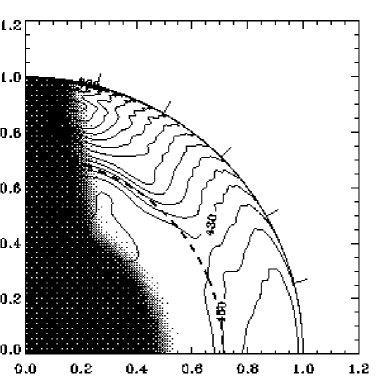
FIG. 17.: Inferred rotation rate $\Omega/2\pi$ in a quadrant of the Sun, obtained by means of SOLA inversion of 144 days of MDI data. The equator is at the horizontal axis and the pole is at the vertical axis, both axes being labelled by fractional radius. Some contours are labelled in nHz, and, for clarity, selected contours are shown as bold. The dashed circle is at the base of the convection zone and the tick marks at the edge of the outer circle are at latitudes $15^{\circ}$, $30^{\circ}$, $45^{\circ}$, $60^{\circ}$, and $75^{\circ}$. The shaded area indicates the region in the Sun where no reliable inference can be made with the current data. (Adapted from Schou et al., 1998.)

Very extensive results on rotational splitting have been obtained in the last few years. These include data from the GONG network in the form of individual frequency splittings, and from the SOI/MDI instrument on SOHO in the form of $a$ coefficients extending as high as $a_{35}$. As discussed in Section VI C 2, these observational developments have been accompanied by the development of efficient inversion algorithms. Schou et al. (1998) carried out analyses of the data from the first 144 days of data from SOI/MDI using a variety of inversion techniques. Figure 17 shows the inferred angular velocity, obtained by means of SOLA inversion. To illustrate some of the features of the solution more clearly, Fig. 18 shows cuts at fixed latitudes. In accordance with the earlier results, the angular velocity depends predominantly on latitude in the convection zone, while there is little significant variation in the radiative interior. The transition between these two regions, denoted the tachocline by Spiegel and Zahn (1992), appears to be quite sharp, and to coincide approximately with the base of the convection zone.

FIG. 18.: Inferred rotation rate $\Omega/2\pi$ as a function of radius at the latitudes indicated, obtained from inversion of 144 days of MDI data. The circles with 1-$\sigma$ error bars show results of a SOLA inversion, while the dashed lines with 1-$\sigma$ error band were obtained with RLS inversion. The heavy vertical dashed line marks the base of the convection zone. (Adapted from Schou et al., 1998.)

The quality of the MDI data is such that finer details in the rotation become very apparent. As was found in earlier analyses, the angular velocity increases with depth beneath the surface, at least at low latitude, the maximum angular velocity occurring on the equator at a depth of around $0.05\,R$. Korzennik et al. (1990), noting the same feature in the equatorial rotation rate, pointed out that this variation could be related to the different rotation rates inferred from tracking of surface features, assuming that these features were anchored at different depths.

The tachocline is of very considerable dynamical interest, as providing the coupling between the latitude-varying rotation in the convection zone and the nearly solid rotation below it. Furthermore, it seems likely that the solar dynamo must operate in this region, with properties that depend sensitively on the details of the variation in angular velocity (e.g., Parker, 1993). The apparent width of the tachocline in Fig. 18 in part reflects the finite resolution of the inversion, as determined by the radial extent of the averaging kernels. This must be taken into account in estimating the true width of the tachocline. Estimates of the width and other properties were made by Kosovichev (1996a) and Corbard et al. (1998a, 1999). Charbonneau et al. (1999) applied several analysis techniques to LOWL data; they obtained a tachocline width of $(0.039\pm 0.013)\,R$ and an equatorial central radius $r_{\rm c}=(0.693\pm 0.002)\,R$, essentially placing the transition beneath the convection zone. As noted previously by Antia et al. (1998) and Di Mauro and Dziembowski (1998), Charbonneau et al. found some indication that $r_{\rm c}$ increased towards the pole, with an equator-to-pole variation of $\Delta r_{\rm c}=(0.024\pm 0.004)\,R$, in the sense that the tachocline is prolate.

Although the overall features of rotation, as presented above, have been found using several different data sets and analysis methods, it should be mentioned that there are problems at the level of finer details, particularly at higher latitudes. These have become apparent in comparisons between results based on data from the GONG and SOI/MDI projects, in both cases analyzed with the procedures used by both projects (e.g., Howe et al., 2001a; Schou et al., 2002). The origin of the differences in the inferred rotation rates can be traced back mainly to differences in the analysis procedures used to determine the oscillation frequencies from the spherical-harmonic-filtered time series (cf. Section VI B 2). Also, as illustrated by the comparison of the SOLA and RLS results in Fig. 18, different inversion methods may give different results at high latitude. Clearly, the underlying causes for these various differences, and how to correct for them, need to be identified.

As discussed in Section IV C, models of solar evolution have suggested the possible existence in the present Sun of a rapidly rotating core. Thus it is of obvious interest to infer the properties of rotation close to the solar center. Unfortunately, this is extremely difficult and the results obtained so far are somewhat contradictory. Only for modes of the lowest degrees do the kernels extend into the core and even for these the contribution from the core to the rotational splitting is small. In addition, the observational determination of the splitting is difficult at low degree: here only a few values of $m$ are available, the total splitting may be comparable to the natural widths of the peaks in the oscillation power spectra, and the common procedures for frequency determination may introduce a systematic bias (Appourchaux et al., 2000b). A review of the problems in determining the core rotation, and of the results, was given by Eff-Darwich and Korzennik (1998). As a result of the small contribution from the core to the splitting, even fairly modest differences in the observed splittings of low-degree modes can give disparate results for the core rotation. Indeed, recent published values range from somewhat higher than the surface rotation rate (e.g., Gizon et al., 1997; Corbard et al., 1998b), over rates consistent with the bulk of the envelope (e.g., Lazrek et al., 1996) to rotation substantially below the surface rate (e.g., Elsworth et al., 1995b; Tomczyk, Schou, and Thompson, 1995). Charbonneau et al. (1998) showed, based on LOWL data, that a core of radius $0.1R$ could rotate at no more than twice the surface rate. Chaplin et al. (1999b) attempted to obtain averages of rotation localized to the core, from a combination of BiSON and LOWL splittings. The results were consistent with constant rotation of the radiative interior, although with a possible suggestion of a down-turn in the core; analysis of the averaging kernels showed that constraining the measure of rotation to the inner 20 % of the solar radius was only possible at the expense of very substantial errors in the inferred rotation rate. Results consistent with uniform rotation of the deep interior were also obtained by Chaplin et al. (2001a) who made a careful simulation of possible systematic errors in the determination of the low-degree frequency splittings.

IX The changing, aspherical Sun

The Sun is not a static object. The slow evolutionary changes are likely too small to be detectable within a human lifetime; however, the changes associated with the 22-year solar magnetic cycle (cf. Section IV D) may be expected to influence the structure and dynamics of the solar interior with measurable consequences for the oscillation frequencies. One may hope that this can provide information about the inner workings of the magnetic cycle, including the possible dynamo mechanisms responsible for it. In particular, dynamo action just below the convection zone might produce organized magnetic fields of sufficient strength to be detectable in the oscillation frequencies.

The first evidence for frequency changes was obtained by Woodard and Noyes (1985) who found an average decrease in frequencies of low-degree modes of around $0.42\,\mu{\rm Hz}$ from 1980 (close to solar maximum) to 1984 (near solar minimum). More extensive data by Libbrecht and Woodard (1990, 1991), covering a substantial range in frequency and degree, confirmed the general trend and provided information about the dependence of the frequency change on mode parameters. It was found that the change largely scaled as the inverse mode inertia, much as do the effects of near-surface errors (cf. Section V B). From 1986 to 1989 (i.e., essentially from minimum to close to maximum) the frequencies increased by up to around $0.8\,\mu{\rm Hz}$; the change varied strongly with frequency, from being negligible below $1.5\,{\rm mHz}$ to a maximum at $4\,{\rm mHz}$. On this basis it was concluded that the dominant source of the frequency variation was localized very close to the solar surface. This was confirmed in a careful comparison of results from several different data sets by Chaplin et al. (2001b). Furthermore, the frequency variations have been shown to be closely correlated with surface activity, even on time scales of months (e.g., Woodard et al., 1991; Bachmann and Brown, 1993; Rhodes et al., 1993; Elsworth et al., 1994; Chaplin et al., 2001c).

A closely related issue are the effects of departures from spherical symmetry. The resulting variations in wave speed with latitude make a contribution to the frequency splitting in azimuthal order that is independent of the sign of $m$; thus, in terms of the expansion given in Eq. (78) these effects give rise to even $a$ coefficients. Early measurements of these coefficients were reported by Duvall et al. (1986) and Brown and Morrow (1987). These coefficients, and their variation during the solar cycle, behaved in a manner corresponding to the time-varying latitude dependence of the solar surface temperature and magnetic field (e.g., Kuhn, 1988; Goode and Kuhn, 1990; Woodard and Libbrecht, 1993). Extensive data during the rising phase of the present solar cycle have been obtained from the GONG and SOI/MDI experiments, greatly strengthening the evidence for a close correlation between the variations in the oscillation frequencies and the surface magnetic field (Dziembowski et al., 1998, 2000; Howe et al., 1999). Antia et al. (2001) considered data covering the period 1995–2000 from both GONG and SOI/MDI, and extending to $a_{14}$. They again found a very close correlation between the variations in the $a$ coefficients and in the corresponding components of a Legendre-polynomial expansion of the surface magnetic flux; this strongly suggests that the behavior of the oscillation frequencies is directly related to the near-surface magnetic field. Furthermore, from an inverse analysis of the changes they confirmed the superficial nature of the changes in the wave-propagation speed.

From these results it may appear that the measurements of the frequency changes and the even $a$ coefficients have so far added little to our knowledge about solar variability. Nonetheless, it is still of considerable interest to investigate the causes for these effects. Gough and Thompson (1988) concluded that the asphericities causing the even $a$ coefficients in the expansion of frequency splittings were likely of magnetic origin. Goldreich et al. (1991) carried out an analysis of the effects of changes in the near-surface magnetic field and the entropy of the convection zone and similarly concluded that the dominant cause of the frequency change with time was magnetic. A subsequent analysis by Balmforth et al. (1996) confirmed that entropy perturbations alone were unlikely to be able to account for the observed frequency changes.

The frequency changes for low-degree modes generally follow the same behavior as seen at high degrees (e.g., Elsworth et al., 1994). However, closer inspection reveals striking differences: Jiménez-Reyes et al. (1998) found that, when plotted against magnetic flux, the frequency changes exhibited hysteresis, with the frequency at a given flux being larger during the rising phase of the solar cycle than during the declining phase. Moreno-Insertis and Solanki (2000) showed that this behavior could be understood in terms of the variation with phase of the solar cycle of the distribution of the magnetic field over the solar surface, as could variations in the frequency change with degree. This behavior is clearly closely related to the changes in the even $a$ coefficients during the solar cycle, discussed above.

According to Eq. (59) the f-mode frequencies are determined essentially by the solar surface radius. This has been used to estimate corrections to the commonly used value by comparing the observed frequencies to those of solar models (Schou et al., 1997; Antia, 1998). Dziembowski et al. (1998) and Antia et al. (2000a) noted that the inferred radius changed with time, reflecting possible solar-cycle changes in the solar surface radius. However, it was pointed out by Dziembowski et al. (2001) that, as already noted by Gough (1993), Eq. (59) should be corrected for the finite radial extent of the f-mode eigenfunctions; thus the inferred radius change may in fact take place in subsurface layers, resulting from changes in magnetic fields or temperature stratification, with little effect on the photospheric radius $R_{\rm ph}$. Dziembowski et al. (2001) concluded that the change in $R_{\rm ph}$ associated with the solar cycle is only a few kilometres, of uncertain sign, and hence certainly too small to have a significant effect on the solar irradiance.

Although the evidence discussed so far points to a superficial nature of the effects of solar activity on solar structure and oscillation frequencies, it is possible that magnetic fields, or other aspherical perturbations, sufficiently strong to have an observable effect may exist deeper within the Sun. Gough et al. (1996b) carried out inversion of even $a$ coefficients to search for radial variations of the asphericity, concluding that it was confined to a shallow layer close to the surface. Antia et al. (2000b) found evidence for an aspherical perturbation at $r\simeq 0.96R$; by analyzing frequencies of modes penetrating beyond the base of the convection zone they also placed an upper limit of around 30 Tesla on a possible toroidal magnetic field located in this region. Evidence for asphericity in the wave speed over a range of depths in the convection zone was also found by Dziembowski et al. (2000). Finally, from analysis of SOI/MDI data Antia et al. (2001) found a significant peak, at $r=0.92R$ and a latitude of $60^{\circ}$, in the time-averaged asphericity, with a similar though weaker signal in GONG data. The physical nature of these perturbations is so far unknown; in particular, as shown by Zweibel and Gough (1995) it is very difficult to distinguish between direct magnetic effects and effects of variations in the sound speed.

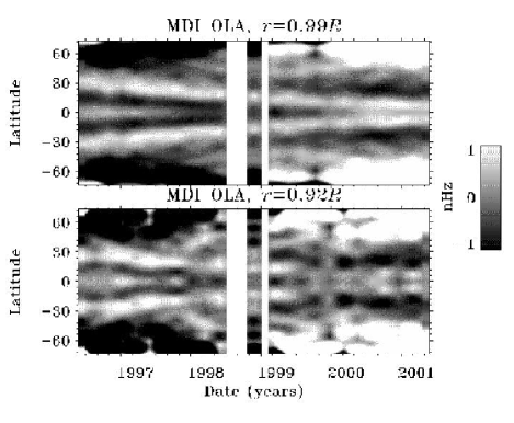
FIG. 19.: The evolution with time in the zonal flows, inferred from SOLA inversions of data from SOI/MDI, after subtraction of the time-averaged rotation rate. The results are presented as a function of time and latitude, the grey scale at the right giving the scale in nHz. The top panel is at a radius of $0.99R$ and the bottom panel is at $0.92R$. Note that the plot has been symmetrized around the equator, since global rotational inversion only senses the symmetrical component of the rotation rate (cf. Section V E). The white vertical stripes correspond to periods where the SOHO spacecraft was temporarily non-functional. (Adapted from Howe et al., 2001b.)

Solar activity also affects the dynamics of the solar convection zone. In Doppler observations of the solar surface Howard and LaBonte (1980) found bands of slightly faster and slower rotation, which they called torsional oscillations, shifting towards lower latitudes as the solar cycle progressed (for more recent results, see Ulrich, 1998, 2001). Kosovichev and Schou (1997) and Schou et al. (1998) found similar variations with latitude in the rotation rate inferred from helioseismic inversion, extending over perhaps 5 % of the solar radius. By analyzing f-mode frequency splittings, Schou (1999) showed that these bands shifted towards the equator with time, in a manner very similar to the surface torsional oscillations. Howe et al. (2000a, 2001b) studied the depth variation and time evolution of these so-called zonal flows, as illustrated in Fig. 19. Here data from SOI/MDI have been analyzed in 72-day segments, to infer the rotation rate during each of these periods; an average over all segments over time, at each latitude and radial location, has been subtracted, and the resulting residuals are displayed. The bands of faster rotation converging towards the equator are evident. Remarkably, these can be followed below the surface to a depth of at least 8 % of the solar radius; on the solar surface, they correspond closely to the variations first seen by Howard and LaBonte. Thus these variations involve a substantial fraction of the solar convection zone. Similar results were obtained by Antia and Basu (2000, 2001). Vorontsov et al. (2002) analyzed SOI/MDI data using an adaptive regularization technique and found indications that the flows involve the entire convection zone. The physical origin of these zonal flows is as yet not clear; it is interesting, however, that Covas et al. (2000) found a similar spatial and temporal behavior of rotation in a mean-field dynamo model of the solar magnetic variations.

Birch and Kosovichev (1998) and Schou et al. (1998) found that the near-polar rotation was substantially slower than expected from the directly observed surface rotation rate (cf. Eq. 1) or from a simple extrapolation from results at lower latitude. Similarly, Fig. 19 shows substantial variations at higher latitudes, not obviously related to the zonal flows at lower latitude. These variations can be followed to latitudes of at least $80^{\circ}$ (Schou, 1999; Antia and Basu, 2001).

FIG. 20.: Deviation from the mean rotation rate inferred from inversions at various locations near the base of the convection zone, as a function of time. Open circles represent results from the GONG network, and filled triangles are from the SOI/MDI experiment. (From Howe et al., 2001b.)

Variations in the rotation rate at even greater depth were detected by Howe et al. (2000b; see also Howe et al., 2001b). These are illustrated in Fig. 20, which again is based on subtracting time-averaged rotation rates from the results for time segments. The most striking variation, seen both in data from GONG and SOI/MDI, is an oscillation with a period of around 1.3 y in the equatorial region at the base of the convection zone. Careful analyses have shown that this cannot simply be an effect of systematic errors in the observations with an annual period. At the depth of $0.63R$, well below the convection zone, there are indications of an oscillation with the same period but the opposite phase. Significant variations are also found at higher latitude, although with less regular periodicities. Possible physical mechanisms that may be responsible for this behavior were discussed by Thompson (2001); a particularly interesting model results from dynamo calculations which exhibit period-halving bifurcations (Covas et al., 2001).

X Local helioseismology

So far, I have considered global modes of solar oscillation, resulting from the interference of acoustic or surface-gravity waves travelling through the Sun. The frequencies of these modes reflect the properties, such as structure and rotation, of that part of the Sun through which travel the waves making up a given mode. By suitably combining the frequencies of these modes, information about structure and rotation can be localized to limited regions in radius and latitude, providing inferences about the variation of these properties with position within the Sun.

Powerful though they are, such analyses have obvious limitations. The global modes extend over all longitudes; thus analysis of their frequencies provide essentially no information about longitude variation of solar properties; furthermore, as discussed in Section V E, they depend only on that component of, e.g., rotation which is symmetric around the equator. Also, the properties of global modes have little sensitivity to meridional or more complex flows, such as large-scale convective eddies, which may be present in the solar convection zone. Further, although the modes are undoubtedly affected by sunspots or other manifestations of strong localized magnetic fields, these effects do not lend themselves to detailed inferences of, say the three-dimensional subsurface structure of a sunspot.

However, it is possible to analyse the observations in ways that provide more general information. The wave field in a given region of the solar surface is affected by the properties of that region, including the subsurface layers down to the depth of penetration, determined by the lower turning point (cf. Eq. 41) of the waves that are observed. By analyzing the properties of such local waves, it is possible to infer local three-dimensional structures and flows beneath the solar surface.

Early investigations of this nature considered the wave field around sunspots. By carrying out a so-called Hankel transform of the waves in cylindrical coordinates, centered on the spot, Braun, Duvall & LaBonte (1987) demonstrated that wave energy was absorbed or scattered by the spot. This provided the potential for studying the subsurface structure of active regions. Brown (1990) presented a technique for inverting such data to obtain a map of active-region structure; he noted that, unlike ‘classical’ helioseismology using oscillations frequencies, this is based on observations of amplitudes and phases of the waves. A detailed review of the seismology of active regions was given by Bogdan & Braun (1995).

Studies of local properties of the solar interior, known as local helioseismology, are developing very rapidly, although they have not yet reached the level of maturity of global helioseismology. A basic difficulty which has not yet been fully solved is the treatment of the forward problem, i.e., the calculation of the wave field and the resulting observables for a given subsurface structure and flow. (In contrast, in global helioseismology it is straightforward to compute oscillation frequencies for a solar model with an assumed rotation law.) As a result, the inferences made through local analysis are somewhat difficult to interpret, in terms of their resolution and the extent to which they reflect the true properties of the solar interior, although substantial progress has recently been made in this area.

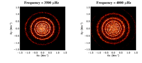
FIG. 21.: Ring diagrams obtained as cuts through tri-dimensional power spectra at the frequencies indicated; the data used are SOI/MDI full-disc Dopplergrams. Each ring corresponds to a value of the radial order $n$. (Adapted from González Hernández et al. 1998a.)

A Ring-diagram analysis

Possibly the first analysis of effects on oscillation frequencies of local perturbations was presented by Gough and Toomre (1983). They pointed out that the frequencies would be changed by a local velocity field, through the advection of the wave pattern; furthermore, they established the frequency perturbation resulting from a local perturbation to the sound speed. This suggestion was developed into a practical procedure by Hill (1988). He considered the power spectrum, based on the oscillation field over a restricted area of the solar surface, as a function of frequency $\omega$ and the components $k_{x}$ and $k_{y}$ of the horizontal wave vector in the longitude and latitude directions. In the $(\omega,k_{x},k_{y})$ space the results are ‘trumpet-like’ surfaces, obtained by rotating the ridges in Fig. 10 around the frequency axis. The analysis is carried out by considering cuts through these surfaces at fixed frequency: the result is a set of rings, each corresponding to a ridge in the $l-\nu$ diagram. (cf. Fig. 21). As shown by Hill (1988) these rings are shifted by the underlying horizontal flow field, the shift of a given ring being given by an average of the velocity weighted by the relevant radial eigenfunction. Similarly, variations in the subsurface sound speed cause a distortion of the rings. Thus, by considering different rings and different frequencies, a set of data is obtained from which the depth variation of the flow or the sound speed can be inferred by means of inversion techniques such as those described in Section VI C. These results are then assumed to represent horizontal averages over the region for which the ring diagrams have been determined. By repeating this for several regions on the solar surface, a map of the flow and subsurface sound speed can be built up.

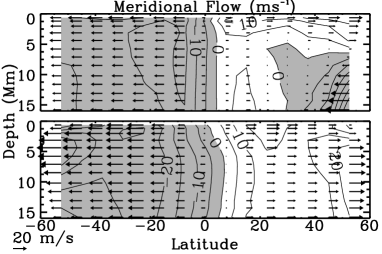
FIG. 22.: Meridional flows in the solar convection zone, as inferred from ring-diagram analysis, plotted against latitude (abscissa) and depth beneath the solar surface (ordinate). The length of the arrows indicate the speed, the scale being indicated at the lower left; grey regions mark southward flow. The results in the lower panel were obtained in 1997, at relatively low solar activity, whereas the upper panel is from 2001, close to solar maximum activity. (Adapted from Haber et al., 2002.)

Detailed analyses have been carried out of the flows in the solar convection zone by means of this technique. Clear evidence has been found for meridional flows, which tend to be poleward at periods of low solar activity (e.g., González Hernández et al., 1998b; Haber et al., 1998, 2000; Schou and Bogart, 1998; Basu, Antia, and Tripathy, 1999). At higher activity, the situation appears to be more complicated. Some recent results, from an extensive analysis of MDI data by Haber et al. (2002), are illustrated in Fig. 22. In the lower panel, obtained near solar minimum, there is a regular flow from the equator towards the poles at all depths. In the upper panel, however, obtained near solar maximum activity, the flows in the Northern hemisphere are substantially more complicated, a countercell with an equator-ward flow having developed at depth at higher latitudes.

The ring-diagram analysis also allows separate determination of the rotation rate in the northern and southern hemispheres. Haber et al. (2000, 2001) found zonal flows converging towards the equator, similar to those inferred from global helioseismic inversions (cf. Section IX), although with a substantial North-South asymmetry, as illustrated in Fig. 23. When symmetrized around the equator, these results were in reasonable agreement with those obtained from global inversions, however.

FIG. 23.: Longitudinally averaged zonal flows, obtained from ring-diagram analysis. The dashed curves show results at a depth of 0.9 Mm, and the solid curves are at a depth of 7 Mm. The results in the lower panel were obtained in 1997, at relatively low solar activity, whereas the upper panel is from 2001, close to solar maximum activity. This should be compared to the zonal flows obtained from global analysis (cf. Fig. 19); note that in the latter figure only the component symmetrical around the equator is obtained. (Adapted from Haber et al., 2001.)

Hindman et al. (2001) used ring diagrams to determine what essentially corresponds to the mean multiplet frequency, as a function of position on the solar disk, and in this way obtained local frequency shifts associated with active regions; when averaged over the solar disk and time, the results are not inconsistent with the frequency changes observed for global modes over the solar cycle (cf. Section IX). This may provide insight into the physical origins of these frequency changes. A related theoretical investigation of frequency shifts caused by localized strong magnetic fields, such as are present in active regions, was carried out by Cunha et al. (1998).

B Time-distance analysis and helioseismic holography

In geoseismology the most commonly used procedure is to measure the travel time for waves between a known source and a detector. The sources range from distant earthquakes, in investigations of the global structure of the Earth, to vibrators in measurements of local subsurface structures. The travel time provides an integral of the wave speed along the path of the wave; many such travel times can be combined to produce a coherent model of the region under study. In this way it has been possible to obtain a three-dimensional model of the interior of the Earth (e.g., Dziewonski and Woodhouse, 1987).

In the solar case there are no similarly sharply defined sources of the waves: as discussed in Section V F, the waves are continuously excited by the random effects of the near-surface convection. Nevertheless, it was argued by Duvall et al. (1993b) that a similar signal could be obtained from a suitable correlation analysis of the wave field observed at the solar surface; the time delay maximizing the correlation between two points provides a measure of the travel time along the ray connecting these two points. The technique was developed further by D’Silva (1996) and D’Silva et al. (1996). Within the approximation of geometrical acoustics the travel time along the ray $\Gamma_{i}$ can be written as

$$\tau_{i}(t)=\int_{\Gamma_{i}}{{\rm d}s\over c_{\rm w}({\bf r},t)+{\bf v}({\bf r},t)\cdot{\bf n}}\;,$$ (95)

where $s$ is distance along the ray, ${\bf r}$ is the spatial coordinate, $c_{\rm w}$ is the local wave speed, ${\bf v}$ is the local flow velocity and ${\bf n}$ is a unit vector along the ray; the appearance of time $t$ indicates that both the wave speed and flow velocity may depend on time. The wave speed is predominantly given by the sound speed but may be perturbed by magnetic fields in active regions. Given measurements along a sufficient number of rays, these relations may be inverted to infer $c_{\rm w}({\bf r},t)$ and ${\bf v}({\bf r},t)$ (Kosovichev, 1996b). Reviews of time-distance techniques were given by Kosovichev and Duvall (1997), and Kosovichev et al. (2000, 2001).

In practice, the correlation analysis is carried out between regions of the solar surface, typically a small central area and a surrounding ring or parts of a ring. Also, Eq. (95) assumes that the waves can be treated in the ray approximation. It was noted by Bogdan (1997) that this approximation is questionable in the solar case, since the wavelength in general is not small compared to the scale of the features that are investigated. Birch and Kosovichev (2000, 2001) studied the effects of wave-speed perturbations in the first Born approximation to derive travel-time sensitivity kernels, relating the wave-speed perturbation to the change in the travel time, as a replacement for the ray approximation. Jensen et al. (2000) proposed simple analytical approximations to such kernels and showed that they were in reasonable agreement with sensitivity computations based on solutions to the wave equation. These kernels were used for inversion to infer wave-speed perturbations by Jensen et al. (2001), who also determined averaging kernels reflecting the resolution properties of the inversion. Birch et al. (2001) made a careful analysis of the accuracy of the Born and ray approximations, by comparing them with direct calculations of the scattering of acoustic waves in a uniform medium. Finally, Jensen and Pijpers (2002) derived sensitivity kernels for wave-speed perturbations and flow velocity in the Rytov approximation, and compared various approximations to these kernels. It is very encouraging that the theoretical basis for the time-distance technique is getting more solidly established through these analyses; information transfer from similar work in geophysics has been very fruitful in this regard.

Time-distance analyses have been used to investigate the near-surface flow fields associated with supergranular convection (e.g., Kosovichev, 1996b). In an interesting analysis based on f modes, Duvall and Gizon (2000) evaluated the vertical vorticity associated with the flow and showed that this was in agreement with theoretical expectations for convection in a rotating system. Giles et al. (1997) determined properties of the meridional flows in the solar convection zone, from the equator towards the poles, also seen with the ring-diagram analyses (cf. Fig. 22). Inferences of meridional flows over an an extended range of depths within the convection zone were reported by Duvall and Kosovichev (2001); interestingly, no evidence was found for a return flow. Variations with time in the meridional flow, inferred from time-distance analysis, were discussed by Chou and Dai (2001). As in the ring-diagram results, the flow showed increasing complexity with increasing solar activity; however, as Chou and Dai did not carry out an inversion in the radial direction, a more detailed comparison of the results is not possible.

Investigations have also been made of wave-speed perturbations associated with emerging active regions (e.g., Kosovichev et al., 2000; Jensen et al., 2001). An example is shown in Fig. 24. It is evident that the emerging magnetic field is associated with a complex structure of generally increased wave speed below the solar surface. Zhao et al. (2001) recently inferred the velocity field beneath a large sunspot; they found a strong mass flow across the spot at depth of 9–12 Mm, indicating that the magnetic field responsible for the spot has a rather loose structure at these depths.

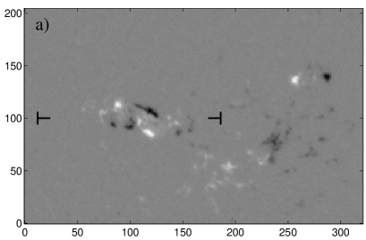
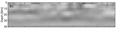
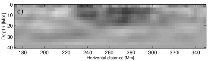
FIG. 24.: Panel (a) shows an MDI magnetogram of an emerging active region; distances are in Mm, and the black and white regions indicate magnetic fields of opposite polarity, over a range between $-0.1$ and $0.1$ Tesla. Panels (b) and (c) show wave-speed perturbations below the surface, at the cross section marked by $\vdash$ and $\dashv$ in panel (a); the grey scale ranges from perturbations of $-0.2\,{\rm km}\,{\rm s}^{-1}$ (white) to $0.5\,{\rm km}\,{\rm s}^{-1}$ (black). Panel (c) was obtained at the same time as the magnetogram in panel (a), while panel (b) was taken 16 hours earlier. (Adapted from Jensen et al., 2001.)

A technique closely related to time-distance helioseismology is known as helioseismic holography. It goes back to a proposal by Roddier (1975) to use holographic methods to visualize acoustic sources below the solar surface, followed by a suggestion by Lindsey and Braun (1990) that it might be possible to form an acoustic image of sunspots on the back of the Sun. However, the first practical application of the technique seems to have been by Lindsey and Braun (1997) and the parallel development of the so-called technique of acoustic imaging by Chang et al. (1997). In these techniques, the acoustic wave field on the solar surface is combined coherently, taking into account the phase information, to reconstruct the presence of acoustic absorbers or scatterers in the subsurface layers. The methods have predominantly been used to investigate the subsurface structure and acoustic properties of active regions (e.g., Chen et al., 1998; Braun et al., 1998; Lindsey and Braun, 1998; Braun and Lindsey, 2000). A tutorial review of helioseismic holography was given by Lindsey and Braun (2000a), while Chou (2000) reviewed the work done on acoustic imaging. A technique for inversion of the holographic data was presented by Skartlien (2002).

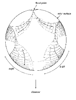
FIG. 25.: Schematic illustration of the principle in imaging active regions on the far side of the Sun. The figure shows the propagation of waves in a cross section of the Sun, starting from a focal point in an active region on the far side and observed in the pupil on the near side. See text for details. (Adapted from Lindsey and Braun, 2000b.)

The ability of the holographic analysis to detect active regions on the far side of the Sun was convincingly demonstrated by Lindsey and Braun (2000b), through analysis of data from SOI/MDI. The principle is illustrated schematically in Fig. 25. Waves emerging from the far side of the Sun can be measured on the near side, in the region denoted ‘pupil’, after one or more reflections at the solar surface; through appropriate analysis of the measured wave field it is possible to focus on specific regions on the far side. Relative to the neighboring quiet photosphere waves from the active region suffer a phase shift which can be detected. This is illustrated in Fig. 26 where the phase shift (expressed as a change in travel time) determined on the far side is compared to a magnetogram of the same region after it has moved to the near side of the Sun as a result of solar rotation. There is clearly a striking agreement between the features in the acoustic and direct image. Further developments of this technique has allowed imaging of the entire far side of the Sun, extending also to the region near the solar limb and over the poles (Braun and Lindsey 2001).

I finally mention that Woodard (2002) has developed a new analysis method where the intermediate steps between data and inferences are to some extent bypassed, hence approaching the ideal case presented in the introduction to Section VI B. Specifically, he obtained a relation between inhomogeneity-induced correlations in the observed wave field and the underlying supergranular flow. Results of analysis of data from the MDI instrument showed a very promising correlation with the directly measured surface flow field. A detailed comparison of this technique with other techniques of local helioseismology, evaluating its advantages and possible disadvantages, still remains to be carried out, however.

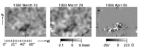
FIG. 26.: The leftmost two panels show travel-time perturbations $\Delta t$, in the vicinity of an active region on the far side of the Sun. The right-hand panel shows a magnetogram of the same region 10 days later, after the region has become visible on the near side. The rule indicates angular distance on the solar surface. (Adapted from Lindsey and Braun, 2000b.)

XI The helioseismic Sun

It seems unlikely that even the most optimistic predictions in the early phases of helioseismology, around 1975, could have foreseen the extent to which the solar interior can now be probed. Inferences of solar structure have shown that standard calculations of solar models reproduce the actual structure to a precision better than 0.5 % in sound speed. This is a remarkable demonstration of the ability of physics, including our current understanding of the microscopic properties of matter under stellar conditions, to predict properties of such a relatively complex object as the Sun. It also provides strong evidence that the discrepancy between the predicted and measured capture rates of neutrinos results from the properties of the neutrinos, rather than from errors in the modeling of the solar interior. Indeed, the strong constraints on solar structure from helioseismology provide a basis for using the solar core as a well-calibrated neutrino source for the study of neutrino physics. The solar rotation rate has been determined in much of the solar interior, revealing striking variations with position, and changes in time. Further, information is emerging about the flows in the solar convection zone and the subsurface structure of magnetically active regions.

These are remarkable achievements, in providing observational information about the internal properties of a star. However, an important goal is now to understand the results in physical terms, and evaluate their broader consequences for the modeling of stellar structure and evolution, as well as their implications for our understanding of physics of matter in stars.

Investigations of the thermodynamic properties in the convection zone have shown that even the present complex descriptions are inadequate, at the level of precision reached by the helioseismic inferences; this demonstrates the possibility of using the Sun as a laboratory for the study of the equation of state of partially ionized matter, in very great detail. Although the effects are subtle in the solar case, they could have substantial importance under other astrophysical circumstances, such as in lower-mass stars or giant planets where the interactions between the constituents of the plasma are much stronger.

The successes in overall solar modeling should not overshadow the failures: the differences between the inferred solar sound speed and the predictions of the models are far larger than the observational uncertainty. A particularly striking feature is the localized region just below the convection zone where the solar sound speed is substantially higher than that of the models. This is a region where the models predict a strong gradient in the hydrogen abundance, as a result of settling of helium from the convection zone towards the interior. It also approximately coincides with the tachocline, i.e., the transition between the latitudinally varying rotation in the convection zone and the almost uniform rotation in the radiative interior. It was suggested by Gough and McIntyre (1998) that the uniform rotation of the interior is maintained by a weak magnetic field, the tachocline being established as a boundary layer; within this region circulation is established which leads to mixing. Mixing would also result from the strongly anisotropic turbulence originally suggested by Spiegel and Zahn (1992) to explain the tachocline. In either case, mixing of the region just beneath the convection zone would tend to reduce the composition gradients, locally increasing the hydrogen abundance and hence the sound speed, as required by the helioseismic results (Brun et al., 1999; Elliott and Gough, 1999). Such smoothing of the gradient was also suggested by the inversions, discussed in Section VII B, for the hydrogen abundance.

Independent evidence for mixing beneath the convection zone comes from the reduction in the solar photospheric lithium abundance, relative to the primordial value (cf. Section III). Lithium is destroyed by nuclear reactions at temperatures above $2.5\times 10^{6}\,{\rm K}$, substantially higher than the temperature at the base of the convection zone. In fact, models with mixing have been computed which match the lithium abundance, suppressing also the peak in the sound-speed difference just below the convection zone (e.g., Richard et al., 1996; Chaboyer, 1998; Brun et al., 1999). On the other hand, the fact that the photospheric beryllium abundance is close to the primordial value indicates that significant mixing does not extend to temperatures as high as $3.5\times 10^{6}\,{\rm K}$ where beryllium is destroyed.

The inferences of solar internal rotation show that the rotation rate is almost constant in the radiative interior: unlike simple models of the Sun’s rotational evolution from an assumed state of rapid initial rotation, there is no indication of a rapidly rotating core. An important consequence is that the solar oblateness, which can be calculated precisely from the inferred rotation rate, has no significant effects on tests, based on planetary motion, of Einstein’s theory of general relativity (e.g., Pijpers, 1998; Roxburgh, 2001). The nearly uniform rotation of the radiative interior indicates the presence of efficient transport of angular momentum, coupling the radiative interior to the convection zone, from which angular-momentum loss has taken place through the solar wind. It was proposed by Kumar and Quataert (1997) and Talon and Zahn (1998) that angular-momentum transport might take place by means of gravity waves generated at the base of the solar convection zone. However, Gough and McIntyre (1998), with reference to analogous phenomena in the Earth’s atmosphere, argued that gravity waves would be unlikely to have the required effect; they identified magnetic effects as the only plausible transport mechanism, a weak primordial field being sufficient to ensure the required coupling.

The variation of the rotation rate in the convection zone, reflected also in the latitude dependence observed on the solar surface, is presumably maintained by angular-momentum redistribution within the convection zone, through interaction between rotation, convection and possibly other flows. The observed variation is inconsistent with relatively simple models which tend to predict a rotation rate depending on the distance to the rotation axis (cf. Section IV C). It was pointed out by Gough (1976) that the interaction between rotation and small-scale convection might lead to an anisotropic turbulent viscosity which could affect angular-momentum transport; an estimate of the anisotropic Reynolds stress tensor was made on the basis of three-dimensional hydrodynamical simulations by Pulkkinen et al. (1993). Pidatella et al. (1986) used simple models of this nature to interpret early helioseismic inferences of rotation in the convection zone. Recently, the numerical resolution in full hydrodynamical simulations of the solar convection zone has become sufficient to capture at least some aspects of the smaller-scale turbulence (e.g., Miesch, 2000; Miesch et al., 2000; Brun and Toomre, 2002); the results of these simulations show an encouraging similarity to the helioseismically inferred rotation profile.

It is likely that interaction between convection and rotation is responsible for the formation of the large-scale solar magnetic field and its 22-year variation in the solar magnetic cycle, through some kind of dynamo mechanism. Dynamo models have in fact been constructed which are based on the helioseismically inferred rotation rate (e.g., Parker, 1993; Charbonneau and MacGregor, 1997).

Analyses of data during the period leading to the present maximum in solar activity have shown striking variations in solar rotation. Zonal flows converging towards the solar equator, previously detected in surface observations, have been shown to extend over a substantial fraction of the convection zone. These bands of somewhat faster and slower rotation appear to be related to the equator-ward drift of locations of sunspots as the solar cycle progresses (e.g., Howard and LaBonte, 1980; Snodgrass, 1987; Ulrich, 1998, 2001); however, the physical connection is as yet not understood. Even more surprising has been the detection of oscillations with a period of 1.3 y in the rotation rate near and below the base of the convection zone; one may hope that they can provide additional information about conditions in this region and possibly about the mechanism of the solar dynamo. It is evident that such temporal variations provide strong arguments for further detailed observations of solar oscillations, ideally through at least one full 22-year magnetic cycle.

Further information about the detailed structure and dynamics of the convection zone has been obtained from local helioseismology. Large-scale convective flow patterns have been detected, as well as meridional flows with complex structure that appears to depend on the level of magnetic activity. This may lead to a detailed understanding of the mechanisms controlling convection and rotation, including the angular-momentum transport, when the observations are combined with the increasingly realistic modeling of the dynamics of the solar convection zone. Also, detailed information is becoming available about the subsurface structure and time evolution of active regions, which will likely lead to a better understanding of the processes underlying their formation. Particularly interesting is the detection of active regions on the far side of the Sun; by giving advance warning before they reach the near side 1 – 2 weeks later and hence have the potential to unleash eruptions in the direction of the Earth, such observations may be helpful in reducing the risk of harmful effects from such eruptions.

The causes of the solar oscillations are not central to the use of the frequencies for helioseismic investigations, although the processes responsible for the excitation and damping undoubtedly contribute to the frequency shifts, suppressed in inverse analyses, which are induced by the superficial layers of the Sun. The statistical properties of the observed modes seem largely to be consistent with stochastic excitation of damped oscillations, as discussed in Section V F (e.g., Chaplin et al., 1997; Chang and Gough, 1998). Furthermore, Stein and Nordlund (1998b, 2001) showed that hydrodynamical simulations of solar near-surface convection predicted the excitation of oscillations, with an energy input approximately consistent with the observations; a detailed comparison by Georgobiani et al. (2000) between observations and hydrodynamical simulations of solar oscillations also showed overall agreement, including indications of asymmetry. On this basis, we can be reasonably confident that we understand the overall aspects of the excitation of the solar modes; thus it may be possible to use the observed properties of the oscillations, including the statistics of the amplitudes, to obtain information about convection beneath the solar surface.

XII Per aspera ad astra

Although impressive advances have been made on the helioseismic study of the solar interior, this provides information about only an individual, relatively simple star. Complete testing of the theory of stellar structure and evolution would require studies of the broad range of stellar types, spanning very different physical properties and processes, that are observed. These include effects, such as rapid rotation or convective cores, that cannot be investigated in the solar case. Fortunately, it has been found that stars of very different types, covering most stellar masses and evolutionary states, show pulsations; often, these stars are multi-mode pulsators and hence in principle offer relatively detailed information about their interiors. For example, such stars include the $\gamma$ Doradus and $\delta$ Scuti stars, the slowly pulsating B stars and the $\beta$ Cephei stars, which span the main sequence from masses of $1.5$ to more than 10 solar masses, and various classes of white dwarfs. Thus there would appear to be an excellent potential for asteroseismology, probing the stellar interiors on the basis of the observed frequencies.

In most cases, the oscillations are caused by intrinsic driving resulting from various radiative or perhaps convective mechanisms. Although modes may be unstable in a substantial range of frequencies, the modes observed are typically only a relatively small subset of the unstable modes, and the selection of modes which reaches observable amplitudes is complex and poorly understood. As a result, it is difficult to identify the observed frequencies with specific modes, characterized by their degree, radial and azimuthal order; this has severely limited the possibilities for using the modes for investigating the stellar interiors.

In contrast, oscillations excited in a manner similar to what is observed in the Sun are expected to show a broad spectrum of observable modes, most modes in this range being present since no subtle selections are at work in the determination of the mode amplitudes. This makes solar-like oscillations very attractive for asteroseismology. Furthermore, the relation between stellar structure and the oscillation frequencies is relatively well understood. In the foreseeable future stellar observations will be restricted to disk-averaged data, and hence to low-degree modes; however, as discussed in Section V C 3 these are precisely the modes that give information about the properties of stellar cores.

On the basis of our understanding of the source of the solar oscillations (see Section XI), one may expect similar oscillations in other stars with outer convection zones, although the predictions of their amplitudes are still somewhat uncertain (e.g., Christensen-Dalsgaard and Frandsen, 1983; Houdek et al., 1999). However, in any case the expected amplitudes in main-sequence stars is extremely low, as is also observed in the solar case: the predicted velocity amplitudes are typically below $1\,{\rm m}\,{\rm s}^{-1}$ and the relative luminosity amplitudes are below around 10 parts per million, severely stretching the capabilities of ground-based observations faced with instrumental problems and fluctuations in the Earth’s atmosphere. Thus it is hardly surprising that the observational results until recently have been at best tentative. An extensive co-ordinated campaign with most of the World’s then largest telescopes (Gilliland et al., 1993) failed to find oscillations in stars in the open cluster M67, in some cases with upper limits below the theoretical predictions. Promising results were obtained by Brown et al. (1991) and Martić et al. (1999) for Procyon, again with amplitudes somewhat below predictions. Detailed results for the sub-giant $\eta$ Bootis were obtained by Kjeldsen et al. (1995); interestingly, modeling by Christensen-Dalsgaard et al. (1995) and Guenther and Demarque (1996) showed that there might be evidence for g-mode-like behavior in the observed frequencies. However, it must be noted that the observations were questioned by Brown et al. (1997).

FIG. 27.: Power spectrum of oscillations of $\alpha$ Cen A, from radial-velocity observations with the CORALIE fiber-fed echelle spectrograph on the 1.2 m Swiss telescope at the La Silla site of the European Southern Observatory. (From Bouchy and Carrier, 2001.)

In the last few years the observational situation has undergone a dramatic improvement. Interesting results have been obtained from photometric observations with the star tracker on the otherwise failed WIRE satellite (e.g., Buzasi et al., 2000; Schou and Buzasi, 2001). Furthermore, techniques have been developed for very stable radial-velocity measurements in connection with the search for extra-solar planets. This has resulted in the detection of evidence for solar-like oscillations in the star $\beta$ Hydri (Bedding et al., 2001); also, as shown in Fig. 27, a very clear detection has been made in the ‘solar twin’ $\alpha$ Centauri A (Bouchy and Carrier, 2001).

Further developments are expected of ground-based observing facilities, including the HARPS spectrograph (Queloz et al., 2001) to be installed on the 3.6 m telescope of the European Southern Observatory at La Silla. A major breakthrough of asteroseismology of solar-like stars will result from observations from space. The Canadian MOST satellite (for Microvariability and Oscillations of STars; Matthews 1998) will be launched late in 2002. The French COROT satellite (for COnvection, ROtation and planetary Transits; Baglin et al. 1998, 2002) is scheduled for launch in 2004, and will obtain very extended time series, with correspondingly high frequency resolution, for a handful of stars. Two other projects are under development. The Danish Rømer satellite is being developed, with the MONS project (for Measuring Oscillations in Nearby Stars; Christensen-Dalsgaard 2002), with launch planned for 2005; this will be in an orbit that allows access to stars in essentially the entire sky. Finally, the Eddington mission (Favata, 2002) currently has the status as reserve mission in the programme of the European Space Agency; it will carry out precise measurements of oscillations of a large number of stars of a variety of types.

Data for distant stars will obviously never be as detailed as those that have been obtained for the Sun; however, there is no doubt that asteroseismic investigations of a broad range of stars, with very different properties, will contribute greatly to our understanding of stellar structure and evolution over the coming decades.

REFERENCES

- [1] Abdurashitov, J. N., T. J. Bowles, M. L. Cherry, et al., 1999, “Measurement of the solar neutrino capture rate by SAGE and implications for neutrino oscillations in vacuum,” Phys. Rev. Lett. 83, 4686–4689.
- [2] Abrams, D., and P. Kumar, 1996, “Asymmetries of solar -mode line profiles,” Astrophys. J. 472, 882–890.
- [3] Adelberger, E. G., S. M. Austin, J. N. Bahcall, et al., 1998, “Solar fusion cross sections,” Rev. Mod. Phys. 70, 1265–1291.
- [4] Aerts, C., T. R. Bedding, and J. Christensen-Dalsgaard, (eds), 2002, Proc. IAU Colloq. 185: Radial and nonradial pulsations as probes of stellar physics, ASP Conf. Ser., vol. 259 (ASP, San Francisco), p. i–xxvii, 1–667.
- [5] Ahmad, Q. R., R. C. Allen, T. C. Andersen, et al., 2001, “Measurement of the rate of interactions produced by solar neutrinos at the Sudbury Neutrino Observatory,” Phys. Rev. Lett. 87, 071301–(1-6).
- [6] Allende Prieto, C., D. L. Lambert, and M. Asplund, 2001, “The forbidden abundance of oxygen in the Sun,” Astrophys. J. 556, L63–L66.
- [7] Anders, E., and N. Grevesse, 1989, “Abundances of the elements: meteoritic and solar,” Geochim. Cosmochim. Acta 53, 197–214.
- [8] Anderson, E. R., T. L. Duvall, Jr., and S. M. Jefferies, 1990, “Modeling of solar oscillation power spectra,” Astrophys. J. 364, 699–705.
- [9] Ando, H., and Y. Osaki, 1975, “Nonadiabatic nonradial oscillations: An application to the five-minute oscillation of the sun,” Publ. Astron. Soc. Japan 27, 581–603.
- [10] Angulo, C., M. Arnould, M. Rayet, et al., 1999, “A compilation of charged-particle induced thermonuclear reaction rates,” Nucl. Phys. A 656, 3–183.
- [11] Antia, H. M., 1998, “Estimate of the solar radius from f-mode frequencies,” Astron. Astrophys. 330, 336–340.
- [12] Antia, H. M., and S. Basu, 1994a, “Nonasymptotic helioseismic inversion for solar structure,” Astron. Astrophys. Suppl. Ser. 107, 421–444.
- [13] Antia, H. M., and S. Basu, 1994b, “Measuring the helium abundance in the solar envelope: the role of the equation of state,” Astrophys. J. 426, 801–811.
- [14] Antia, H. M., and S. Basu, 2000, “Temporal variations of the rotation rate in the solar interior,” Astrophys. J. 541, 442–448.
- [15] Antia, H. M., and S. Basu, 2001, “Temporal variations of the solar rotation rate at high latitudes,” Astrophys. J. 559, L67–L70.
- [16] Antia, H. M., S. Basu, and S. M. Chitre, 1998, “Solar internal rotation rate and the latitudinal variation of the tachocline,” Mon. Not. R. Astron. Soc. 298, 543–556.
- [17] Antia, H. M., S. Basu, F. Hill, R. Howe, R. W. Komm, and J. Schou, 2001, “Solar-cycle variation of the sound-speed asphericity from GONG and MDI data 1995–2000,” Mon. Not. R. Astron. Soc. 327, 1029–1040.
- [18] Antia, H. M., S. Basu, J. Pintar, and B. Pohl, 2000a, “Solar cycle variation in solar f-mode frequencies and radius,” Solar Phys. 192, 459–468.
- [19] Antia, H. M., and S. M. Chitre, 1997, “Helioseismic models and solar neutrino fluxes,” Mon. Not. R. Astron. Soc. 289, L1–L4.
- [20] Antia, H. M., and S. M. Chitre, 1998, “Determination of temperature and chemical composition profiles in the solar interior from seismic models,” Astron. Astrophys. 339, 239–251.
- [21] Antia, H. M., S. M. Chitre, and M. J. Thompson, 2000b, “The Sun’s acoustic asphericity and magnetic fields in the solar convection zone,” Astron. Astrophys. 360, 335–344.
- [22] Appourchaux, T., H.-Y. Chang, D. O. Gough, and T. Sekii, 2000b, “On measuring low-degree p-mode frequency splitting with full-disc integrated data,” Mon. Not. R. Astron. Soc. 319, 365–376.
- [23] Appourchaux, T., C. Fröhlich, B. Andersen, et al., 2000a, “Observational upper limits to low-degree solar -modes,” Astrophys. J. 538, 401–414.
- [24] Appourchaux, T., L. Gizon, and M.-C. Rabello-Soares, 1998, “The art of fitting p-mode spectra. I. Maximum likelihood estimation,” Astron. Astrophys. Suppl. Ser. 132, 107–119.
- [25] Appourchaux, T., M.-C. Rabello-Soares, and L. Gizon, 1998, “The art of fitting p-mode spectra. II. Leakage and noise covariance matrices,” Astron. Astrophys. Suppl. Ser. 132, 121–132.
- [26] Asplund, M., Å. Nordlund, R. Trampedach, and R. F. Stein, 2000b, “Line formation in solar granulation. II. The photospheric Fe abundance,” Astron. Astrophys. 359, 743–754.
- [27] Asplund, M., Å. Nordlund, R. Trampedach, C. Allende Prieto, and R. F. Stein, 2000a, “Line formation in solar granulation. I. Fe line shapes, shifts and asymmetries,” Astron. Astrophys. 359, 729–742.
- [28] Auwers, A., 1891, “Der Sonnendurchmesser und der Venusdurchmesser nach den Beobachtungen an den Heliometern der deutschen Venus-Expedition,” Astron. Nachr. 128, 361–375.
- [29] Böhm-Vitense, E., 1958, “Über die Wasserstoffkonvektionszone in Sternen verschiedener Effektivtemperaturen und Leuchtkräfte,” Z. Astrophys. 46, 108–143.
- [30] Bachmann, K. T., and T. M. Brown, 1993, “-mode frequency variation in relation to global solar activity,” Astrophys. J. 411, L45–L48.
- [31] Backus, G., and F. Gilbert, 1970, “Uniqueness in the inversion of inaccurate gross Earth data,” Phil. Trans. R. Soc. London, Ser. A 266, 123–192.
- [32] Baglin, A. and the COROT team, 1998, “Asteroseismology with the space mission COROT,” in Proc. IAU Symp. 185: New eyes to see inside the Sun and stars, edited by F.-L. Deubner, J. Christensen-Dalsgaard, and D. W. Kurtz (Kluwer, Dordrecht) p. 301–308.
- [33] Baglin, A., M. Auvergne, P. Barge, J.-T. Buey, C. Catala, E. Michel, W. Weiss, and the COROT Team, 2002, “COROT: Asteroseismology and planet finding,” in Proc. 1st Eddington Workshop, ‘Stellar Structure and Habitable Planet Finding’, ESA SP-485, eds F. Favata, I. W. Roxburgh and D. Galadi (ESA Publications Division, Noordwijk, The Netherlands), p. 17–24.
- [34] Bahcall, J. N., 1989, Neutrino astrophysics, (Cambridge University, Cambridge, England).
- [35] Bahcall, J. N., N. A. Bahcall, and G. Shaviv, 1968, “Present status of the theoretical predictions for the solar-neutrino experiment,” Phys. Rev. Lett. 20, 1209–1212.
- [36] Bahcall, J. N., N. A. Bahcall, and R. K. Ulrich, 1968, “Mixing in the Sun and neutrino fluxes,” Astrophys. Lett. 2, 91–95.
- [37] Bahcall, J. N., L. S. Brown, A. Gruzinov, and R. F. Sawyer, 2002, “The Salpeter plasma correction for solar fusion reactions,” Astron. Astrophys. 383, 291–295.
- [38] Bahcall, J. N., and M. H. Pinsonneault, 1992, “Standard solar models, with and without helium diffusion and the solar neutrino problem,” Rev. Mod. Phys. 64, 885–926.
- [39] Bahcall, J. N., and M. H. Pinsonneault (with an appendix by G. J. Wasserburg), 1995, “Solar models with helium and heavy-element diffusion,” Rev. Mod. Phys. 67, 781–808.
- [40] Bahcall, J. N., M. H. Pinsonneault, and S. Basu, 2001, “Solar models: current epoch and time dependences, neutrinos, and helioseismological properties,” Astrophys. J. 555, 990–1012.
- [41] Bahcall, J. N., M. H. Pinsonneault, S. Basu, and J. Christensen-Dalsgaard, 1997, “Are standard solar models reliable?” Phys. Rev. Lett. 78, 171–174.
- [42] Bahcall, J. N., P. I. Krastev, and A. Yu. Smirnov, 1998, “Where do we stand with neutrino oscillations?” Phys. Rev. D 59, 096016–(1-22).
- [43] Bahng, J., and M. Schwarzschild, 1963, “Hydrodynamic oscillations in the solar chromosphere,” Astrophys. J. 137, 901–913.
- [44] Balachandran, S. C., and R. A. Bell, 1998, “Shallow mixing in the solar photosphere inferred from revised beryllium abundances,” Nature (London) 392, 791–793.
- [45] Balmforth, N. J., 1992a, “Solar pulsational stability. I: Pulsation-mode thermodynamics,” Mon. Not. R. Astron. Soc. 255, 603–631.
- [46] Balmforth, N. J., 1992b, “Solar pulsational stability. III: Acoustical excitation by turbulent convection,” Mon. Not. R. Astron. Soc. 255, 639–649.
- [47] Balmforth, N. J., D. O. Gough, and W. J. Merryfield, 1996, “Structural changes to the Sun through the solar cycle,” Mon. Not. R. Astron. Soc. 278, 437–448.
- [48] Bartenwerfer, D., 1973, “Differential rotation, magnetic fields and the solar neutrino flux,” Astron. Astrophys. 25, 455–456.
- [49] Basu, S., 1998, “Effects of errors in the solar radius on helioseismic inferences,” Mon. Not. R. Astron. Soc. 298, 719–728.
- [50] Basu, S., and H. M. Antia, 1995, “Helium abundance in the solar envelope,” Mon. Not. R. Astron. Soc. 276, 1402–1408.
- [51] Basu, S., and H. M. Antia, 1997, “Seismic measurement of the depth of the solar convection zone,” Mon. Not. R. Astron. Soc. 287, 189–198.
- [52] Basu, S., and H. M. Antia, 2001, “A study of possible temporal and latitudinal variations in the properties of the solar tachocline,” Mon. Not. R. Astron. Soc. 324, 498–508.
- [53] Basu, S., H. M. Antia, and D. Narasimha, 1994, “Helioseismic measurement of the extent of overshoot below the solar convection zone,” Mon. Not. R. Astron. Soc. 267, 209–224.
- [54] Basu, S., H. M. Antia, and S. C. Tripathy, 1999, “Ring diagram analysis of near-surface flows in the Sun,” Astrophys. J. 512, 458–470.
- [55] Basu, S., W. J. Chaplin, J. Christensen-Dalsgaard, Y. Elsworth, G. R. Isaak, R. New, J. Schou, M. J. Thompson, and S. Tomczyk, 1997b, “Solar internal sound speed as inferred from combined BiSON and LOWL oscillation frequencies,” Mon. Not. R. Astron. Soc. 292, 243–251.
- [56] Basu, S., and J. Christensen-Dalsgaard, 1997, “Equation of state and helioseismic inversions,” Astron. Astrophys. 322, L5–L8.
- [57] Basu, S., J. Christensen-Dalsgaard, and M. J. Thompson, 1997a, “SVD preprocessing of helioseismic data for solar structure inversion,” Astron. Astrophys. 321, 634–642.
- [58] Basu, S., W. Däppen, and A. Nayfonov, 1999, “Helioseismic analysis of the hydrogen partition function in the solar interior,” Astrophys. J. 518, 985–993.
- [59] Basu, S., M. H. Pinsonneault, and J. N. Bahcall, 2000, “How much do helioseismological inferences depend on the assumed reference model?” Astrophys. J. 529, 1084–1100.
- [60] Basu, S., and M. J. Thompson, 1996, “On constructing seismic models of the Sun,” Astron. Astrophys. 305, 631–642.
- [61] Batchelor, G. K., 1956, The theory of homogeneous turbulence. (Cambridge University, Cambridge, England).
- [62] Baturin, V. A., W. Däppen, D. O. Gough, and S. V. Vorontsov, 2000, “Seismology of the solar envelope: sound-speed gradient in the convection zone and its diagnosis of the equation of state,” Mon. Not. R. Astron. Soc. 316, 71–83.
- [63] Baturin, V. A., and I. V. Mironova, 1990, “On the possibility of determining helium abundance from helioseismological data,” Pis’ma Astron. Zh. 16, 253–259 [Sov. Astron. Lett. 16, 108–111 (1990)].
- [64] Beck, J. G., 2000, “A comparison of differential rotation measurements,” Solar Phys. 191, 47–70.
- [65] Bedding, T. R., R. P. Butler, H. Kjeldsen, I. K. Baldry, S. J. O’Toole, C. G. Tinney, G. W. Marcey, F. Kienzle, and F. Carrier, 2001, “Evidence for solar-like oscillations in beta Hydri,” Astrophys. J. 549, L105–L108.
- [66] Bertello, L., F. Varadi, R. K. Ulrich, C. J. Henney, A. G. Kosovichev, R. A. García, and S. Turck-Chièze, 2000, “Identification of solar acoustic modes of low angular degree and low radial order,” Astrophys. J. 537, L143–L146.
- [67] Berthomieu, G., A. J. Cooper, D. O. Gough, Y. Osaki, J. Provost, and A. Rocca, 1980, “Sensitivity of five minute eigenfrequencies to the structure of the Sun,” in Nonradial and Nonlinear Stellar Pulsation, Lecture Notes in Physics 125, edited by H. A. Hill and W. Dziembowski (Springer, Berlin), p. 307–312.
- [68] Birch, A. C., and A. G. Kosovichev, 1998, “Latitudinal variation of solar subsurface rotation inferred from -mode frequency splittings measured with SOI-MDI and GONG,” Astrophys. J. 503, L187–L190.
- [69] Birch, A. C., and A. G. Kosovichev, 2000, “Travel time sensitivity kernels,” Solar Phys. 192, 193–201.
- [70] Birch, A. C., and A. G. Kosovichev, 2001, “The Born approximation in time-distance helioseismology,” in Proceedings of the SOHO 10 / GONG 2000 Workshop: Helio- and Asteroseismology at the Dawn of the Millennium, ESA SP-464, edited by A. Wilson (ESA Publications Division, Noordwijk, The Netherlands), p. 187–190.
- [71] Birch, A. C., A. G. Kosovichev, G. H. Price, and R. B. Schlottmann, 2001, “The accuracy of the Born and ray approximations in time-distance helioseismology,” Astrophys. J. 561, L229–L232.
- [72] Bogdan, T. J., 1997, “A comment on the relationship between the modal and time-distance formulations of local helioseismology,” Astrophys. J. 477, 475–484.
- [73] Bogdan, T. J., and D. C. Braun, 1995, “Active region seismology,” in Proc. Fourth SOHO Workshop: Helioseismology, ESA SP-376, vol. 1, edited by J. T. Hoeksema, V. Domingo, B. Fleck, and B. Battrick (ESA Publications Division, Noordwijk, The Netherlands), p. 31–45.
- [74] Bouchy, F., and F. Carrier, 2001, “P-mode observations on Cen A,” Astron. Astrophys. 374, L5–L8.
- [75] Boury, A., M. Gabriel, A. Noels, R. Scuflaire, and P. Ledoux, 1975, “Vibrational instability of a 1 star towards non-radial oscillations,” Astron. Astrophys. 41, 279–285.
- [76] Braun, D. C., T. L. Duvall, Jr, and B. J. LaBonte, 1987, “Acoustic absorption by sunspots,” Astrophys. J. 319, L27–L31.
- [77] Braun, D. C., and C. Lindsey, 2000, “Helioseismic holography of active region subphotospheres,” Solar Phys. 192, 285–305.
- [78] Braun, D. C., and C. Lindsey, 2001, “Seismic imaging of the far hemisphere of the Sun,” Astrophys. J. 560, L189–L192.
- [79] Braun, D. C., C. Lindsey, Y. Fan, and M. Fagan, 1998, “Seismic holography of solar activity,” Astrophys. J. 502, 968–980.
- [80] Breger, M., and M. H. Montgomery, (eds), 2000, Delta Scuti and related stars, ASP Conference Series, vol. 210 (ASP, San Francisco), pp. i–xv, 1–582.
- [81] Brodskiǐ, M. A., and A. Levshin, 1977, “Asimptoticheskiy metod opredeleniya skorostnogo razreza Zemli po chastotam yeye sobstvennykh kolebaniy,” Dodl. Akad. Nauk. SSSR 233, 312–315.
- [82] Brodskiǐ, M. A., and S. V. Vorontsov, 1989, “The inverse problem of helioseismology: probing the structure of the lower solar atmosphere,” Pis’ma Astron. Zh. 15, 61–69 [Sov. Astron. Lett. 15, 27–30 (1989)].
- [83] Brodsky, M. A., and S. V. Vorontsov, 1993, “Asymptotic theory of intermediate- and high-degree solar acoustic oscillations,” Astrophys. J. 409, 455–464.
- [84] Brookes, J. R., G. R. Isaak, and H. B. van der Raay, 1976, “Observation of free oscillations of the Sun,” Nature (London) 259, 92–95.
- [85] Brown, T. M., 1984, “The Fourier tachometer II – An instrument for measuring global solar velocity fields,” in Proceedings of Conference on Solar Seismology from Space, JPL Publ. 84 – 84, edited by R. K. Ulrich, J. Harvey, J., E. J. Rhodes, Jr., and J. Toomre (NASA, Pasadena), p. 157–163.
- [86] Brown, T. M., 1985, “Solar rotation as a function of depth and latitude,” Nature (London) 317, 591–594.
- [87] Brown, T. M., 1988, “Techniques for observing solar oscillations,” in Proceedings of IAU Symposium No 123, Advances in helio- and asteroseismology, edited by J. Christensen-Dalsgaard and S. Frandsen (Reidel, Dordrecht), p. 453–465.
- [88] Brown, T. M., 1990, “An inverse method for -mode scattering measurements,” Solar Phys. 128, 133–141.
- [89] Brown, T. M., 1996, “Techniques for observing solar oscillations,” in Proceedings of the VI IAC Winter School “The structure of the Sun”, edited by T. Roca Cortés and F. Sánchez (Cambridge University, Cambridge, England), p. 1–45.
- [90] Brown, T. M., and Christensen-Dalsgaard, J., 1998, “Accurate determination of the solar photospheric radius,” Astrophys. J. 500, L195–L198.
- [91] Brown, T. M., J. Christensen-Dalsgaard, W. A. Dziembowski, P. Goode, D. O. Gough, and C. A. Morrow, 1989, “Inferring the Sun’s internal angular velocity from observed p-mode frequency splittings,” Astrophys. J. 343, 526–546.
- [92] Brown, T. M., R. L. Gilliland, R. W. Noyes, and L. W. Ramsey, 1991, “Detection of possible -mode oscillations of Procyon,” Astrophys. J. 368, 599–609.
- [93] Brown, T. M., E. J. Kennelly, S. G. Korzennik, P. Nisenson, R. W. Noyes, and S. D. Horner, 1997, “A radial velocity search for -mode pulsations in Bootis,” Astrophys. J. 475, 322–327.
- [94] Brown, T. M., and C. A. Morrow, 1987, “Depth and latitude dependence of solar rotation,” Astrophys. J. 314, L21–L26.
- [95] Brown, T. M., R. T. Stebbins, and H. A. Hill, 1978, “Long-period oscillations of the apparent solar diameter: Observations,” Astrophys. J. 223, 324–338.
- [96] Brüggen, M., and D. O. Gough, 1997, “On electrostatic screening of ions in astrophysical plasmas,” Astrophys. J. 488, 867–871.
- [97] Brun, A. S., and J. Toomre, 2002, “Turbulent convection under the influence of rotation: sustaining a strong differential rotation,” Astrophys. J. 570, 865–885.
- [98] Brun, A. S., S. Turck-Chièze, and P. Morel, 1998, “Standard solar models in the light of new helioseismic constraints. I. The solar core,” Astrophys. J. 506, 913–925.
- [99] Brun, A. S., S. Turck-Chièze, and J. P. Zahn, 1999, “Standard solar models in the light of new helioseismic constraints. II. Mixing below the convection zone,” Astrophys. J. 525, 1032–1041. (Erratum: Astrophys. J. 536, 1005).
- [100] Buzasi, D., J. Catanzarite, R. Laher, T. Conrow, D. Shupe, T. N. Gautier III, T. Kreidl, and D. Everett, 2000, “The detection of multimodal oscillations on Ursae Majoris,” Astrophys. J. 532, L133–L136.
- [101] Cacciani, A., and M. Fofi, 1978, “The magneto-optical filter. II. Velocity field measurements,” Solar Phys. 59, 179–189.
- [102] Carpenter, K. G., and C. J. Schrijver, 2000, “A dream of a mission: stellar imager and seismic probe,” Bull. Am. Astron. Soc. 32, 721.
- [103] Castellani, V., S. Degl’Innocenti, G. Fiorentini, M. Lissia, and B. Ricci, 1997, “Solar neutrinos: Beyond standard solar models,” Phys. Rep. 281, 309–398.
- [104] Cattaneo, F., 1997, “The solar dynamo problem,” in SCORe’96: Solar Convection and Oscillations and their Relationship, edited by F. P. Pijpers, J. Christensen-Dalsgaard, and C. S. Rosenthal (Kluwer, Dordrecht), p. 201–222.
- [105] Chaboyer, B., 1998, “Internal rotation, mixing and lithium abundance,” in Proceedings of IAU Symposium No 185: New Eyes to see Inside the Sun and Stars, edited by F.-L. Deubner, J. Christensen-Dalsgaard, and D. W. Kurtz (Kluwer, Dordrecht), p. 25–36.
- [106] Chaboyer, B., P. Demarque, and M. H. Pinsonneault, 1995, “Stellar models with microscopic diffusion and rotational mixing. I. Application to the Sun,” Astrophys. J. 441, 865–875.
- [107] Chandrasekhar, S., 1964, “A general variational principle governing the radial and the non-radial oscillations of gaseous masses,” Astrophys. J. 139, 664–674.
- [108] Chang, H.-K., D.-Y. Chou, B. LaBonte, and the TON Team, 1997, “Ambient acoustic imaging in helioseismology,” Nature (London) 389, 825–827.
- [109] Chang, H.-Y., and D. O. Gough, 1998, “On the power distribution of solar p modes,” Solar Phys. 181, 251–263.
- [110] Chaplin, W. J., and T. Appourchaux, 1999, “Depth of excitation and reversal of asymmetry of low- solar p modes: a complementary analysis of BiSON and VIRGO/SPM data,” Mon. Not. R. Astron. Soc. 309, 761–768.
- [111] Chaplin, W. J., T. Appourchaux, Y. Elsworth, G. R. Isaak, and R. New, 2001b, “The phenomenology of solar-cycle-induced acoustic eigenfrequency variations: a comparative and complementary analysis of GONG, BiSON and VIRGO/LOI data,” Mon. Not. R. Astron. Soc. 324, 910–916.
- [112] Chaplin, W. J., J. Christensen-Dalsgaard, Y. Elsworth, R. Howe, G. R. Isaak, R. M. Larsen, R. New, J. Schou, M. J. Thompson, and S. Tomczyk, 1999b, “Rotation of the solar core from BiSON and LOWL frequency observations,” Mon. Not. R. Astron. Soc. 308, 405–414.
- [113] Chaplin, W. J., Y. Elsworth, R. Howe, G. R. Isaak, C. P. McLeod, B. A. Miller, and R. New, 1997, “The observation and simulation of stochastically excited solar p modes,” Mon. Not. R. Astron. Soc. 287, 51–56.
- [114] Chaplin, W. J., Y. Elsworth, R. Howe, G. R. Isaak, C. P. McLeod, B. A. Miller, H. B. van der Raay, S. J. Wheeler, and R. New, 1996, “BiSON performance,” Solar Phys. 168, 1–18.
- [115] Chaplin, W. J., Y. Elsworth, G. R. Isaak, K. I. Marchenkov, B. A. Miller, and R. New, 2001a, “Rigid rotation of the solar core? On the reliable extraction of low- rotational p-mode splittings from full-disc observations of the Sun,” Mon. Not. R. Astron. Soc. 327, 1127–1136.
- [116] Chaplin, W. J., Y. Elsworth, G. R. Isaak, K. I. Marchenkov, B. A. Miller, and R. New, 2001c, “Changes to low- solar p-mode frequencies over the solar cycle: correlations on different time-scales,” Mon. Not. R. Astron. Soc. 322, 22–30.
- [117] Chaplin, W. J., Y. Elsworth, G. R. Isaak, B. A. Miller, and R. New, 1999a, “Skew-symmetric solar modes in low- BiSON data,” Mon. Not. R. Astron. Soc. 308, 424–430.
- [118] Charbonneau, P., J. Christensen-Dalsgaard, R. Henning, R. M. Larsen, J. Schou, M. J. Thompson, and S. Tomczyk, 1999, “Helioseismic constraints on the structure of the solar tachocline,” Astrophys. J. 527, 445–460.
- [119] Charbonneau, P., and K. B. MacGregor, 1997, “Solar interface dynamos. II. Linear, kinematic models in spherical geometry,” Astrophys. J. 486, 502–520.
- [120] Charbonneau, P., S. Tomczyk, J. Schou, and M. J. Thompson, 1998, “The rotation of the solar core inferred by genetic forward modeling,” Astrophys. J. 496, 1015–1030.
- [121] Chen, H.-R., D.-Y. Chou, H.-K. Chang, M.-T. Sun, S.-J. Yeh, B. LaBonte, and the TON Team, 1998, “Probing the subsurface structure of active regions with the phase information in acoustic imaging,” Astrophys. J. 501, L139–L144.
- [122] Chou, D.-Y., 2000, “Acoustic imaging of solar active regions,” Solar Phys. 192, 241–259.
- [123] Chou, D.-Y., and D.-C. Dai, 2001, “Solar cycle variations of subsurface meridional flows in the Sun,” Astrophys. J. 559, L175–L178.
- [124] Chou, D.-Y., M.-T. Sun, T.-Y. Huang, et al., 1995, “Taiwan Oscillation Network,” Solar Phys. 160, 237–243.
- [125] Choudhuri, A. R., 1990, “On the possibility of an -type dynamo in a thin layer inside the Sun,” Astrophys. J. 355, 733–744.
- [126] Christensen-Dalsgaard, J., 1980, “On adiabatic non-radial oscillations with moderate or large ,” Mon. Not. R. astr. Soc. 190, 765–791.
- [127] Christensen-Dalsgaard, J., 1984, “What will asteroseismology teach us?” in Space Research Prospects in Stellar Activity and Variability, edited by A. Mangeney and F. Praderie (Paris Observatory, Paris), p. 11–45.
- [128] Christensen-Dalsgaard, J., 1988, “A Hertzsprung-Russell diagram for stellar oscillations,” in Proceedings of IAU Symposium No 123, Advances in helio- and asteroseismology, edited by J. Christensen-Dalsgaard and S. Frandsen (Reidel, Dordrecht), p. 295–298.
- [129] Christensen-Dalsgaard, J., 1998, “The ‘standard Sun’. Modelling and helioseismology,” Space Science Review 85, 19–36.
- [130] Christensen-Dalsgaard, J., 2002, “MONS on the Danish Rømer satellite: Measuring Oscillations in Nearby Stars,” in Proc. 1st Eddington Workshop, ‘Stellar Structure and Habitable Planet Finding’, ESA SP-485, eds F. Favata, I. W. Roxburgh and D. Galadi (ESA Publications Division, Noordwijk, The Netherlands), p. 25–34.
- [131] Christensen-Dalsgaard, J., T. R. Bedding, and H. Kjeldsen, 1995, “Modelling solar-like oscillations in Bootis,” Astrophys. J. 443, L29–L32.
- [132] Christensen-Dalsgaard, J., W. Däppen, S. V. Ajukov, et al., 1996, “The current state of solar modeling,” Science 272, 1286–1292.
- [133] Christensen-Dalsgaard, J., F. W. W. Dilke, and D. O. Gough, 1974, “The stability of a solar model to non-radial oscillations,” Mon. Not. R. Astron. Soc. 169, 429–445.
- [134] Christensen-Dalsgaard, J., T. L. Duvall, Jr., D. O. Gough, J. W. Harvey, and E. J. Rhodes, Jr., 1985, “Speed of sound in the solar interior,” Nature (London) 315, 378–382.
- [135] Christensen-Dalsgaard, J., and S. Frandsen, 1983, “Stellar 5 min oscillations,” Solar Phys. 82, 469–486.
- [136] Christensen-Dalsgaard, J., and D. O. Gough, 1976, “Towards a heliological inverse problem,” Nature (London) 259, 89–92.
- [137] Christensen-Dalsgaard, J., and D. O. Gough, 1980a, “Implications of the whole-disk Doppler observations of the Sun,” in Nonradial and Nonlinear Stellar Pulsation, Lecture Notes in Physics 125, edited by H. A. Hill and W. Dziembowski (Springer, Berlin), p. 184–190.
- [138] Christensen-Dalsgaard, J., and D. O. Gough, 1980b, “Is the Sun helium-deficient?” Nature (London) 288, 544–547.
- [139] Christensen-Dalsgaard, J., and D. O. Gough, 1982, “On the interpretation of five-minute oscillations in solar spectrum line shifts,” Mon. Not. R. Astron. Soc. 198, 141–171.
- [140] Christensen-Dalsgaard, J., and D. O. Gough, 2001, “On the dipolar f mode of stellar oscillation,” Mon. Not. R. Astron. Soc. 326, 1115–1121.
- [141] Christensen-Dalsgaard, J., D. O. Gough, and K. G. Libbrecht, 1989, “Seismology of solar oscillation line widths,” Astrophys. J. 341, L103–L106.
- [142] Christensen-Dalsgaard, J., D. O. Gough, and F. Pérez Hernández, 1988, “Stellar disharmony,” Mon. Not. R. Astron. Soc. 235, 875–880.
- [143] Christensen-Dalsgaard, J., D. O. Gough, and M. J. Thompson, 1989, “Differential asymptotic sound-speed inversions,” Mon. Not. R. Astron. Soc. 238, 481–502.
- [144] Christensen-Dalsgaard, J., D. O. Gough, and M. J. Thompson, 1991, “The depth of the solar convection zone,” Astrophys. J. 378, 413–437.
- [145] Christensen-Dalsgaard, J., P. C. Hansen, and M. J. Thompson, 1993, “Generalized singular value decomposition analysis of helioseismic inversions,” Mon. Not. R. Astron. Soc. 264, 541–564.
- [146] Christensen-Dalsgaard, J., H. Kjeldsen, and J. A. Mattei, 2001, “Solar-like oscillations of semiregular variables,” Astrophys. J. 562, L141–L144.
- [147] Christensen-Dalsgaard, J., and F. Pérez Hernández, 1992, “Phase-function differences for stellar acoustic oscillations – I. Theory,” Mon. Not. R. Astron. Soc. 257, 62–88.
- [148] Christensen-Dalsgaard, J., C. R. Proffitt, and M. J. Thompson, 1993, “Effects of diffusion on solar models and their oscillation frequencies,” Astrophys. J. 403, L75–L78.
- [149] Christensen-Dalsgaard, J., and J. Schou, 1988, “Differential rotation in the solar interior,” in Seismology of the Sun & Sun-like Stars, ESA SP-286, edited by V. Domingo and E. J. Rolfe (ESA Publications Division, Noordwijk, The Netherlands), p. 149–153.
- [150] Christensen-Dalsgaard, J., J. Schou, and M. J. Thompson, 1990, “A comparison of methods for inverting helioseismic data,” Mon. Not. R. Astron. Soc. 242, 353–369.
- [151] Christensen-Dalsgaard, J., and M. J. Thompson, 1993, “A preprocessing strategy for helioseismic inversions,” Astron. Astrophys. 272, L1–L4.
- [152] Christensen-Dalsgaard, J., and M. J. Thompson, 1997, “On solar p-mode frequency shifts caused by near-surface model changes,” Mon. Not. R. Astron. Soc. 284, 527–540.
- [153] Claverie, A., G. R. Isaak, C. P. McLeod, H. B. van der Raay, and T. Roca Cortes, 1979, “Solar structure from global studies of the 5-minute oscillation,” Nature (London) 282, 591–594.
- [154] Cleveland, B. T., T. Daily, R. Davis, Jr., J. R. Distel, K. Lande, C. K. Lee, P. S. Wildenhain, and J. Ullman, 1998, “Measurement of the solar electron neutrino flux with the Homestake chlorine detector,” Astrophys. J. 496, 505–526.
- [155] Corbard, T., G. Berthomieu, P. Morel, J. Provost, J. Schou, and S. Tomczyk, 1997, “Solar internal rotation from LOWL data. A 2D regularized least-squares inversion using B-splines,” Astron. Astrophys. 324, 298–310.
- [156] Corbard, T., G. Berthomieu, J. Provost, and P. Morel, 1998a, “Inferring the equatorial solar tachocline from frequency splittings,” Astron. Astrophys. 330, 1149–1159.
- [157] Corbard, T., L. Blanc-Féraud, G. Berthomieu, and J. Provost, 1999, “Non linear regularization for helioseismic inversions. Application for the study of the solar tachocline,” Astron. Astrophys. 344, 696–708.
- [158] Corbard, T., M. P. Di Mauro, T. Sekii, and the GOLF team, 1998b, “The solar internal rotation from GOLF splittings,” in Proceedings of the SOHO 6/GONG 98 Workshop: Structure and dynamics of the interior of the Sun and Sun-like stars, ESA SP-418, edited by S. G. Korzennik and A. Wilson (ESA Publications Division, Noordwijk, The Netherlands), p. 741–746.
- [159] Covas, E., R. Tavakol, and D. Moss, 2001, “Dynamical variations of the differential rotation in the solar convection zone,” Astron. Astrophys. 371, 718–730.
- [160] Covas, E., R. Tavakol, D. Moss, and A. Tworkowski, 2000, “Torsional oscillations in the solar convection zone,” Astron. Astrophys. 360, L21–L24.
- [161] Cowling, T. G., 1941, “The non-radial oscillations of polytropic stars,” Mon. Not. R. Astron. Soc. 101, 367–375.
- [162] Cowling, T. G., and R. A. Newing, 1949, “The oscillations of a rotating star,” Astrophys. J. 109, 149–158.
- [163] Cox, A. N., J. A. Guzik, and R. B. Kidman, 1989, “Oscillations of solar models with internal element diffusion,” Astrophys. J. 342, 1187–1206.
- [164] Craig, I. J. D., and J. C. Brown, 1986, Inverse problems in astronomy: a guide to inversion strategies for remotely sensed data, (Adam Hilger, Bristol).
- [165] Cunha, M., M. Brüggen, and D. O. Gough, 1998, “On solar frequency changes,” in Proceedings of the SOHO 6/GONG 98 Workshop: Structure and dynamics of the interior of the Sun and Sun-like stars, ESA SP-418, edited by S. G. Korzennik and A. Wilson (ESA Publications Division, Noordwijk, The Netherlands), p. 905–910.
- [166] Cuypers, J., 1980, “On the calculation of the frequency splitting of adiabatic nonradial stellar oscillations by slow differential rotation,” Astron. Astrophys. 89, 207–208.
- [167] Däppen, W., 1998, “Microphysics: equation of state,” Space Science Review 85, 49–60.
- [168] Däppen, W., and D. O. Gough, 1986, “Progress report on helium abundance determination,” in Seismology of the Sun and the Distant Stars, edited by D. O. Gough (Reidel, Dordrecht), p. 275–280.
- [169] Däppen, W., D. O. Gough, A. G. Kosovichev, and M. J. Thompson, 1991, “A new inversion for the hydrostatic stratification of the Sun,” in Challenges to Theories of the Structure of Moderate-Mass Stars, Lecture Notes in Physics 388, edited by D. O. Gough and J. Toomre (Springer, Berlin), p. 111–120.
- [170] Däppen, W., and J. A. Guzik, 2000, “Astrophysical equation of state and opacity,” in Variable Stars as Essential Astrophysical Tools, NATO Science Series C, vol. 544, edited by C. İbanoğlu (Kluwer Academic, Dordrecht), p. 177–212.
- [171] Davis, R., Jr., D. S. Harmer, and K. C. Hoffman, 1968, “Search for neutrinos from the Sun,” Phys. Rev. Lett. 20, 1205–1209.
- [172] Delache, P., and P. H. Scherrer, 1983, “Detection of solar gravity mode oscillations,” Nature (London) 306, 651–653.
- [173] Demarque, P., J. G. Mengel, and A. V. Sweigart, 1973, “Rotating solar models with low neutrino flux,” Astrophys. J. 183, 997–1004.
- [174] Deubner, F.-L., 1975, “Observations of low wavenumber nonradial eigenmodes of the Sun,” Astron. Astrophys. 44, 371–375.
- [175] Deubner, F.-L., and D. O. Gough, 1984, “Helioseismology: Oscillations as a diagnostic of the solar interior,” Ann. Rev. Astron. Astrophys. 22, 593–619.
- [176] Di Mauro, M. P., J. Christensen-Dalsgaard, M. C. Rabello-Soares, and S. Basu, 2002, “Inferences on the solar envelope with high-degree modes,” Astron. Astrophys. 384, 666–677.
- [177] Di Mauro, M. P., and W. A. Dziembowski, 1998, “Differential rotation of the solar interior: new helioseismic results by inversion of the SOI-MDI/SOHO data,” Mem. Soc. Astron. Ital. 69, 559–562.
- [178] Dicke, R. H., 1964, “The Sun’s rotation and relativity,” Nature (London) 202, 432–435.
- [179] Dilke, F. W. W., and D. O. Gough, 1972, “The solar spoon,” Nature (London) 240, 262–264 and 293–294.
- [180] Domingo, V., B. Fleck, and A. I. Poland, 1995, “The SOHO mission: an overview,” Solar Phys. 162, 1–37.
- [181] D’Silva, S., 1996, “Theoretical foundations of time-distance helioseismology,” Astrophys. J. 469, 964–975.
- [182] D’Silva, S., T. L. Duvall, Jr., S. M. Jefferies, and J. W. Harvey, 1996, “Helioseismic tomography,” Astrophys. J. 471, 1030–1043.
- [183] Duvall, T. L., Jr., 1982, “A dispersion law for solar oscillations,” Nature (London) 300, 242–243.
- [184] Duvall, T. L., Jr., 1995, “Other groundbased observations,” in Proceedings of the Fourth SOHO Workshop: Helioseismology, ESA SP-376, vol. 1, edited by J. T. Hoeksema, V. Domingo, B. Fleck, and B. Battrick (ESA Publications Division, Noordwijk, The Netherlands), p. 107–111.
- [185] Duvall, T. L., Jr., W. A. Dziembowski, P. R. Goode, D. O. Gough, J. W. Harvey, and J. W. Leibacher, 1984, “The internal rotation of the Sun,” Nature (London) 310, 22–25.
- [186] Duvall, T. L., Jr., and L. Gizon, 2000, “Time-distance helioseismology with f modes as a method for measurement of near-surface flows,” Solar Phys. 192, 177–191.
- [187] Duvall, T. L., Jr., and J. W. Harvey, 1983, “Observations of solar oscillations of low and intermediate degree,” Nature (London) 302, 24–27.
- [188] Duvall, T. L., Jr., J. W. Harvey, and M. A. Pomerantz, 1986, “Latitude and depth variation of solar rotation,” Nature (London) 321, 500–501.
- [189] Duvall, T. L., Jr., S. M. Jefferies, J. W. Harvey, Y. Osaki, and M. A. Pomerantz, 1993a, “Asymmetries of solar oscillation line profiles,” Astrophys. J. 410, 829–836.
- [190] Duvall, T. L., Jr., S. M. Jefferies, J. W. Harvey, and M. A. Pomerantz, 1993b, “Time-distance helioseismology,” Nature (London) 362, 430–432.
- [191] Duvall, T. L., Jr., and A. G. Kosovichev, 2001, “New developments in local area helioseismology,” in Proceedings of IAU Symposium No 203: Recent insights into the physics of the Sun and heliosphere: Highlights from SOHO and other space missions, edited by P. Brekke, B. Fleck, and J. B. Gurman (ASP, San Francisco), p. 159–166.
- [192] Dziembowski, W. A., 1977, “Light and radial velocity variations in a nonradially oscillating star,” Acta Astron. 27, 203–211.
- [193] Dziembowski, W. A., P. R. Goode, M. P. Di Mauro, A. G. Kosovichev, and J. Schou, 1998, “Solar cycle onset seen in SOHO Michelson Doppler Imager seismic data,” Astrophys. J. 509, 456–460.
- [194] Dziembowski, W. A., P. R. Goode, A. G. Kosovichev, and J. Schou, 2000, “Signatures of the rise of cycle 23,” Astrophys. J. 537, 1026–1038.
- [195] Dziembowski, W. A., P. R. Goode, and K. G. Libbrecht, 1989, “The radial gradient in the Sun’s rotation,” Astrophys. J. 337, L53–L57.
- [196] Dziembowski, W. A., P. R. Goode, A. A. Pamyatnykh, and R. Sienkiewicz, 1994, “A seismic model of the Sun’s interior,” Astrophys. J. 432, 417–426.
- [197] Dziembowski, W. A., P. R. Goode, and J. Schou, 2001, “Does the Sun shrink with increasing magnetic activity?” Astrophys. J. 553, 897–904.
- [198] Dziembowski, W. A., A. A. Pamyatnykh, and R. Sienkiewicz, 1990, “Solar model from the helioseismology and the neutrino flux problem,” Mon. Not. R. Astron. Soc. 244, 542–550.
- [199] Dziembowski, W. A., A. A. Pamyatnykh, and R. Sienkiewicz, 1991, “Helium content in the solar convective envelope from helioseismology,” Mon. Not. R. Astron. Soc. 249, 602–605.
- [200] Dziewonski, A. M., and J. H. Woodhouse, 1987, “Global images of the Earth’s interior,” Science 236, 37–48.
- [201] Eff-Darwich, A., and S. G. Korzennik, 1998, “Rotation of the solar core: compatibility of the different data sets available,” in Proceedings of the SOHO 6/GONG 98 Workshop: Structure and dynamics of the interior of the Sun and Sun-like stars, ESA SP-418, edited by S. G. Korzennik and A. Wilson (ESA Publications Division, Noordwijk, The Netherlands), p. 685–692.
- [202] Elliott, J. R., and D. O. Gough, 1999, “Calibration of the thickness of the solar tachocline,” Astrophys. J. 516, 475–481.
- [203] Elliott, J. R., and A. G. Kosovichev, 1998, “The adiabatic exponent in the solar core,” Astrophys. J. 500, L199–L202.
- [204] Elsworth, Y., R. Howe, G. R. Isaak, C. P. McLeod, B. A. Miller, R. New, C. C. Speake, and S. J. Wheeler, 1994, “Solar -mode frequencies and their dependence on solar activity: recent results from the BISON network,” Astrophys. J. 434, 801–806.
- [205] Elsworth, Y., R. Howe, G. R. Isaak, C. P. McLeod, B. A. Miller, R. New, S. J. Wheeler, and D. O. Gough, 1995b, “Slow rotation of the Sun’s interior,” Nature (London) 376, 669–672.
- [206] Elsworth, Y., R. Howe, G. R. Isaak, C. P. McLeod, B. A. Miller, H. B. van der Raay, and S. J. Wheeler, 1995a, “Performance of the BISON network 1981-present,” in Proceedings of GONG’94: Helio- and Astero-seismology from Earth and Space, ASP Conference Series, vol. 76, edited by R. K. Ulrich, E. J. Rhodes, Jr., and W. Däppen (ASP, San Francisco), p. 392–397.
- [207] Elsworth, Y., R. Howe, G. R. Isaak, C. P. McLeod, and R. New, 1990, “Evidence from solar seismology against non-standard solar-core models,” Nature (London) 347, 536–539.
- [208] Evans, J. W., and R. Michard, 1962, “Observational study of macroscopic inhomogeneities in the solar atmosphere. III. Vertical oscillatory motions in the solar photosphere,” Astrophys. J. 136, 493–506.
- [209] Ezer, D., and A. G. W. Cameron, 1968, “Solar spin-down and neutrino fluxes,” Astrophys. Lett. 1, 177–179.
- [210] Faulkner, J., and R. L. Gilliland, 1985, “Weakly interacting, massive particles and the solar neutrino flux,” Astrophys. J. 299, 994–1000.
- [211] Favata, F., 2002, “The Eddington baseline mission,” in Proc. 1st Eddington Workshop, ‘Stellar Structure and Habitable Planet Finding’, ESA SP-485, eds F. Favata, I. W. Roxburgh and D. Galadi (ESA Publications Division, Noordwijk, The Netherlands), p. 3–10.
- [212] Finsterle, W., and C. Fröhlich, 2001, “Low-order modes from VIRGO irradiance data,” Solar Phys. 200, 393–406.
- [213] Fiorentini, G., M. Lissia, and B. Ricci, 1999, “Helioseismic tests of diffusion theory,” Astron. Astrophys. 342, 492–495.
- [214] Fossat, E., 1991, “The IRIS network for full disk helioseismology: Present status of the programme,” Solar Phys. 133, 1–12.
- [215] Fossat, E., and G. Ricort, 1975, “Photospheric oscillations. I. Large scale observations by optical resonance method,” Astron. Astrophys. 43, 243–252.
- [216] Frazier, E. N., 1968, “A spatio-temporal analysis of the velocity fields in the solar photosphere,” Z. Astrophys. 68, 345–356.
- [217] Fröhlich, C., D. A. Crommelynck, C. Wehrli, M. Anklin, S. Dewitte, A. Fichot, W. Finsterle, A. Jiménez, A. Chevalier, and H. Roth, 1997, “In-flight performance of the VIRGO solar irradiance instrument on SOHO,” Solar Phys. 175, 267–286.
- [218] Fröhlich, C., and Ph. Delache, 1984, “Solar gravity modes from ACRIM/SMM irradiance data,” Mem. Soc. Astron. Ital. 55, 99–105.
- [219] Fröhlich, C., J. Romero, H. Roth, et al., 1995, “VIRGO: Experiment for helioseismology and solar irradiance monitoring,” Solar Phys. 162, 101–128.
- [220] Fukuda, S., Y. Fukuda, M. Ishitsuka, et al., 2001, “Solar and hep neutrino measurements from 1258 days of Super-Kamiokande data,” Phys. Rev. Lett. 86, 5651–5655.
- [221] Fukuda, Y., T. Hayakawa, E. Ichihara, et al., 1998, “Measurement of a small atmospheric ratio,” Phys. Lett. B 433, 9–18.
- [222] Gabriel, A. H., J. Charra, G. Grec, et al., 1997, “Performance and early results from the GOLF instrument flown on the SOHO mission,” Solar Phys. 175, 207–226.
- [223] Gabriel, A. H., G. Grec, J. Charra, et al., 1995, “Global oscillations at low frequency from the SOHO mission (GOLF),” Solar Phys. 162, 61–99.
- [224] Gabriel, A. H., S. Turck-Chièze, R. A. García, P. L. Pallé, P. Boumier, S. Thiery, G. Grec, R. K. Ulrich, L. Bertello, T. Roca Cortés, and J.-M. Robillot, 1998, “Search for -mode frequencies in the GOLF oscillations spectrum,” in Proceedings of the SOHO 6/GONG 98 Workshop: Structure and dynamics of the interior of the Sun and Sun-like stars, ESA SP-418, edited by S. G. Korzennik and A. Wilson (ESA Publications Division, Noordwijk, The Netherlands), p. 61–66.
- [225] Gabriel, M., 1993, “On the location of the excitation of solar p-modes,” Astron. Astrophys. 274, 935–939.
- [226] Gabriel, M., 1997, “Influence of heavy element and rotationally induced diffusions on solar models,” Astron. Astrophys. 327, 771–778.
- [227] Gabriel, M., 2000, “Linear interaction between pulsations and convection, scattering and line profiles of solar p-modes,” Astron. Astrophys. 353, 399–408.
- [228] Garaud, P., 2002, “Dynamics of the solar tachocline – I. An incompressible study,” Mon. Not. R. astr. Soc. 329, 1–17.
- [229] García, R. A., C. Régulo, S. Turck-Chièze, L. Bertello, A. G. Kosovichev, A. S. Brun, S. Couvidat, C. J. Henney, M. Lazrek, R. K. Ulrich, and F. Varadi, 2001, “Low-degree low-order solar modes as seen by GOLF on board SOHO,” Solar Phys. 200, 361–379.
- [230] Gavrin, V. N., 2001, “Solar neutrino results from SAGE,” Nucl. Phys. B (Proc. Suppl) 91, 36–43.
- [231] Genovese, C. R., P. B. Stark, and M. J. Thompson, 1995, “Uncertainties for two-dimensional models of solar rotation from helioseismic eigenfrequency splitting,” Astrophys. J. 443, 843–854.
- [232] Georgobiani, D., A. G. Kosovichev, R. Nigam, Å. Nordlund, and R. F. Stein, 2000, “Numerical simulations of oscillation modes of the solar convection zone,” Astrophys. J. 530, L139–L142.
- [233] Giles, P. M., T. L. Duvall, Jr., P. H. Scherrer, and R. S. Bogart, 1997, “A subsurface flow of material from the Sun’s equator to its poles,” Nature (London) 390, 52–54.
- [234] Gilliland, R. L., T. M. Brown, H. Kjeldsen, J. K. McCarthy, M. L. Peri, J. A. Belmonte, I. Vidal, L Cram, Palmer E., J., S. Frandsen, M. Parthasarathy, L. Petro, H. Schneider, P. B. Stetson, and W. W. Weiss, 1993, “A search for solar-like oscillations in the stars of M67 with CCD ensemble photometry on a network of 4 m telescopes,” Astron. J. 106, 2441–2476.
- [235] Gilliland, R. L., J. Faulkner, W. H. Press, and D. N. Spergel, 1986, “Solar models with energy transport by weakly interacting particles,” Astrophys. J. 306, 703–709.
- [236] Gilman, P. A., 1986, “The solar dynamo: observations and theories of solar convection, global circulation, and magnetic fields,” in Physics of the Sun, Vol. 1, edited by P. A. Sturrock, T. E. Holzer, D. Mihalas, and R. K. Ulrich (Reidel, Dordrecht), p. 95–160.
- [237] Gilman, P. A., and J. Miller, 1986, “Nonlinear convection of a compressible fluid in a rotating spherical shell,” Astrophys. J. Suppl. Ser. 61, 585–608.
- [238] Gilman, P. A., C. A. Morrow, and E. E. DeLuca, 1989, “Angular momentum transport and dynamo action in the Sun: implications of recent oscillation measurements,” Astrophys. J. 338, 528–537.
- [239] Gizon, L., E. Fossat, M. Lazrek, et al., 1997, “New IRIS constraints on the solar core rotation,” Astron. Astrophys. 317, L71–L74.
- [240] Glatzmaier, G., 1985, “Numerical simulations of stellar convective dynamos. II. Field propagation in the convection zone,” Astrophys. J. 291, 300–307.
- [241] Goldreich, P., and D. A. Keeley, 1977, “Solar seismology. II. The stochastic excitation of the solar -modes by turbulent convection,” Astrophys. J. 212, 243–251.
- [242] Goldreich, P., and P. Kumar, 1990, “Wave generation by turbulent convection,” Astrophys. J. 363, 694–704.
- [243] Goldreich, P., N. Murray, and P. Kumar, 1994, “Excitation of solar -modes,” Astrophys. J. 424, 466–479.
- [244] Goldreich, P., N. Murray, G. Willette, and P. Kumar, 1991, “Implications of solar -mode frequency shifts,” Astrophys. J. 370, 752–762.
- [245] Gong, Z., W. Däppen, and L. Zejda, 2001, “MHD equation of state with relativistic electrons,” Astrophys. J. 546, 1178–1182.
- [246] González Hernández, I., J. Patrón, R. S. Bogart, and the SOI Ring Diagrams Team, 1998a, “Synoptic map of the subsurface velocity flow,” in Proceedings of the SOHO 6/GONG 98 Workshop: Structure and dynamics of the interior of the Sun and Sun-like stars, ESA SP-418, edited by S. G. Korzennik and A. Wilson (ESA Publications Division, Noordwijk, The Netherlands), p. 587–595.
- [247] González Hernández, I., J. Patrón, R. S. Bogart, and the SOI Ring Diagrams Team, 1998b, “Meridional flows from ring diagram analysis,” in Proceedings of the SOHO 6/GONG 98 Workshop: Structure and dynamics of the interior of the Sun and Sun-like stars, ESA SP-418, edited by S. G. Korzennik and A. Wilson (ESA Publications Division, Noordwijk, The Netherlands), p. 781–786.
- [248] Goode, P. R., W. A. Dziembowski, S. G. Korzennik, and E. J. Rhodes, Jr., 1991, “What we know about the Sun’s internal rotation from solar oscillations,” Astrophys. J. 367, 649–657.
- [249] Goode, P. R., and J. R. Kuhn, 1990, “Consistency in trends in helioseismic data and photospheric temperature data through the solar cycle,” Astrophys. J. 356, 310–314.
- [250] Gough, D. O., 1976, “The current state of stellar mixing-length theory,” in Proceedings of IAU Colloquium No. 38: Problems of stellar convection, Lecture Notes in Physics 71, edited by E. A. Spiegel and J.-P. Zahn (Springer, Berlin), p. 15–56.
- [251] Gough, D. O., 1977a, “Mixing-length theory for pulsating stars,” Astrophys. J. 214, 196–213.
- [252] Gough, D. O., 1977b, “Random remarks on solar hydrodynamics,” in Proceedings of IAU Colloquium No. 36: The energy balance and hydrodynamics of the solar chromosphere and corona, edited by R. M. Bonnet and P. Delache (G. de Bussac, Clairmont-Ferrand), p. 3–36.
- [253] Gough, D. O., 1981, “A new measure of the solar rotation,” Mon. Not. R. Astron. Soc. 196, 731–745.
- [254] Gough, D. O., 1982, “A review of the theory of solar oscillations and its implications concerning the internal structure of the Sun,” in Pulsations in Classical and Cataclysmic Variable Stars, edited by J. P. Cox and C. J. Hansen (JILA, Boulder), p. 117–137.
- [255] Gough, D. O., 1984a, “On the rotation of the Sun,” Phil. Trans. R. Soc. London, Ser. A 313, 27–38.
- [256] Gough, D. O., 1984b, “Towards a solar model,” Mem. Soc. Astron. Ital. 55, 13–35.
- [257] Gough, D. O., 1986, “EBK quantization of stellar waves,” in Hydrodynamic and magnetohydrodynamic problems in the Sun and stars, edited by Y. Osaki (Department of Astronomy, University of Tokyo, Tokyo), p. 117–143.
- [258] Gough, D. O., 1990, “Comments on helioseismic inference,” in Progress of Seismology of the Sun and Stars, Lecture Notes in Physics 367, edited by Y. Osaki and H. Shibahashi (Springer, Berlin), p. 283–318.
- [259] Gough, D. O., 1993, “Course 7. Linear adiabatic stellar pulsation,” in Les Houches Session XLVII: Astrophysical fluid dynamics, edited by J.-P. Zahn and J. Zinn-Justin (Elsevier, Amsterdam), p. 399–560.
- [260] Gough, D., 1996a, “Testing solar models: the inverse problem,” in Proceedings of the VI IAC Winter School “The structure of the Sun”, edited by T. Roca Cortés and F. Sánchez (Cambridge University, Cambridge, England), p. 141–228.
- [261] Gough, D. O., 1996b, “Astereoasteroseismology,” Observatory 116, 313–315.
- [262] Gough, D. O., 2001a, “Lessons learned from solar oscillations,” in Astrophysical Ages and Time Scales, ASP Conference Series, vol. 245, edited by T. von Hippel, C. Simpson, and N. Manset, (ASP, San Francisco), p. 31–43.
- [263] Gough, D. O., 2001b, “Inhomogeneity in the solar core,” Solar Phys. 200, 297–303.
- [264] Gough, D. O., 2001c, “The new era in helioseismology,” in Proceedings of IAU Symposium No 203: Recent insights into the physics of the Sun and heliosphere: Highlights from SOHO and other space missions, edited by P. Brekke, B. Fleck, and J. B. Gurman (ASP, San Francisco), p. 3–20.
- [265] Gough, D. O., and A. G. Kosovichev, 1990, “Using helioseismic data to probe the hydrogen abundance in the solar core,” in Proceedings of IAU Colloquium No 121, Inside the Sun, edited by G. Berthomieu and M. Cribier (Kluwer, Dordrecht), p. 327–340.
- [266] Gough, D. O., A. G. Kosovichev, J. Toomre, et al., 1996b, “The seismic structure of the Sun,” Science 272, 1296–1300.
- [267] Gough, D. O., and M. E. McIntyre, 1998, “Inevitability of a magnetic field in the Sun’s radiative interior,” Nature (London) 394, 755–757.
- [268] Gough, D. O., and E. Novotny, 1990, “Sensitivity of solar eigenfrequencies to the age of the Sun,” Solar Phys. 128, 143–160.
- [269] Gough, D. O., and T. Sekii, 2002, “On the effect of error correlation on linear inversion,” Mon. Not. R. Astron. Soc., in the press.
- [270] Gough, D. O., T. Sekii, and P. B. Stark, 1996a, “Inferring spatial variation of solar properties from helioseismic data,” Astrophys. J. 459, 779–791.
- [271] Gough, D. O., and M. J. Thompson, 1988, “On the implications of the symmetric component of the frequency splitting reported by Duvall, Harvey and Pomerantz,” in Proceedings of IAU Symposium No 123, Advances in helio- and asteroseismology, edited by J. Christensen-Dalsgaard and S. Frandsen (Reidel, Dordrecht), p. 175–180.
- [272] Gough, D. O., and M. J. Thompson, 1990, “The effect of rotation and a buried magnetic field on stellar oscillations,” Mon. Not. R. astr. Soc. 242, 25–55.
- [273] Gough, D. O., and M. J. Thompson, 1991, “The inversion problem,” in Solar interior and atmosphere, Space Science Series, edited by A. N. Cox, W. C. Livingston, and M. Matthews (University of Arizona Press, Tucson), p. 519–561.
- [274] Gough, D. O., and J. Toomre, 1983, “On the detection of subphotospheric convective velocities and temperature fluctuations,” Solar Phys. 82, 401–410.
- [275] Gough, D. O., and S. V. Vorontsov, 1995, “Seismology of the solar envelope: measuring the acoustic phase shift generated in the outer layers,” Mon. Not. R. Astron. Soc. 273, 573–582.
- [276] Gough, D. O., and N. O. Weiss, 1976, “The calibration of stellar convection theories,” Mon. Not. R. astr. Soc. 176, 589–607.
- [277] Grec, G., E. Fossat, and M. Pomerantz, 1980, “Solar oscillations: full disk observations from the geographic South Pole,” Nature (London) 288, 541–544.
- [278] Grevesse, N., and A. Noels, 1993, “Cosmic abundances of the elements,” in Origin and evolution of the Elements, edited by N. Prantzos, E. Vangioni-Flam, and M. Cassé (Cambridge University, Cambridge, England), p. 15–25.
- [279] Grevesse, N., and A. J. Sauval, 1998, “Standard solar composition,” Space Science Review 85, 161–174.
- [280] Gruzinov, A. V., and J. N. Bahcall, 1998, “Screening in thermonuclear reaction rates in the Sun,” Astrophys. J. 504, 996–1001.
- [281] Guenther, D. B., 1989, “Age of the Sun,” Astrophys. J. 339, 1156–1159.
- [282] Guenther, D. B., 1994, “Nonadiabatic nonradial -mode frequencies of the standard solar model, with and without helium diffusion,” Astrophys. J. 422, 400–411.
- [283] Guenther, D. B., and P. Demarque, 1996, “Seismology of Bootis,” Astrophys. J. 456, 798–810.
- [284] Guenther, D. B., Y.-C. Kim, and P. Demarque, 1996, “Seismology of the standard solar model: tests of diffusion and the OPAL and MHD equations of state,” Astrophys. J. 463, 382–390.
- [285] Guzik, J. A., and A. N. Cox, 1991, “Effects of opacity and equation of state on solar structure and oscillations,” Astrophys. J. 381, 333–340.
- [286] Guzik, J. A., C. Neuforge-Verheecke, A. C. Young, R. I. Epstein, F. M. Poulin, and J. R. Schissel, 2001, “Standard and non-standard solar models,” Solar Phys. 200, 305–321.
- [287] Haber, D. A., B. W. Hindman, J. Toomre, R. S. Bogart, and F. Hill, 2001, “Development of multiple cells in meridional flows and evolution of mean zonal flows from ring-diagram analyses,” in Proceedings of the SOHO 10 / GONG 2000 Workshop: Helio- and Asteroseismology at the Dawn of the Millennium, ESA SP-464, edited by A. Wilson (ESA Publications Division, Noordwijk, The Netherlands), p. 213–218.
- [288] Haber, D. A., B. W. Hindman, J. Toomre, R. S. Bogart, R. M. Larsen, and F. Hill, 2002, “Evolving submerged meridional circulation cells within the upper convection zone revealed by ring-diagram analysis,” Astrophys. J. 570, 855–864.
- [289] Haber, D. A., B. W. Hindman, J. Toomre, R. S. Bogart, J. Schou, and F. Hill, 1998, “Subphotospheric convective flows determined by ring-diagram analyses of SOI-MDI observations,” in Proceedings of the SOHO 6/GONG 98 Workshop: Structure and dynamics of the interior of the Sun and Sun-like stars, ESA SP-418, edited by S. G. Korzennik and A. Wilson (ESA Publications Division, Noordwijk, The Netherlands), p. 791–796.
- [290] Haber, D. A., B. W. Hindman, J. Toomre, R. S. Bogart, M. J. Thompson, and F. Hill, 2000, “Solar shear flows deduced from helioseismic dense-pack samplings of ring diagrams,” Solar Phys. 192, 335–350.
- [291] Hampel, W., J. Handt, G. Heusser, J. Kiko, et al., 1999, “GALLEX solar neutrino observations: results from GALLEX IV,” Phys. Lett. B 447, 127–133.
- [292] Hansen, C. J., J. P. Cox, and H. M. van Horn, 1977, “The effects of differential rotation on the splitting of nonradial modes of stellar oscillation,” Astrophys. J. 217, 151–159.
- [293] Hansen, P. C., 1990, “Truncated singular value decomposition solutions to discrete ill-posed problems with ill-determined numerical rank,” SIAM J. Sci. Stat. Comp. 11, 503–518.
- [294] Hansen, P. C., 1994, “The Backus-Gilbert method: SVD analysis and fast implementation,” Inverse Problems 10, 895–904.
- [295] Hart, A. B., 1954, “Motions in the Sun at the photospheric level. IV. The equatorial rotation and possible velocity fields in the photosphere,” Mon. Not. R. Astron. Soc. 114, 17–38.
- [296] Hart, A. B., 1956, “Motions in the Sun at the photospheric level. VI. Large scale motions in the equatorial region,” Mon. Not. R. Astron. Soc. 116, 38–55.
- [297] Harvey, J. W., F. Hill, R. P. Hubbard, et al., 1996, “The Global Oscillation Network Group (GONG) project,” Science 272, 1284–1286.
- [298] Haxton, W. C., 1995, “The solar neutrino problem,” Ann. Rev. Astron. Astrophys. 33, 459–503.
- [299] Hill, F., 1988, “Rings and trumpets - three-dimensional power spectra of solar oscillations,” Astrophys. J. 333, 996–1013.
- [300] Hill, F., P. B. Stark, R. T. Stebbins, et al., 1996, “The solar acoustic spectrum and eigenmode parameters,” Science 272, 1292–1295.
- [301] Hill, H. A., R. T. Stebbins, and T. M. Brown, 1976, “Recent oblateness observations: Data, interpretation and significance for earlier work,” in Atomic Masses and Fundamental Constants, vol. 5, edited by J. H. Sanders and A. H. Wapstra (Plenum Press, New York), p. 622–628.
- [302] Hindman, B., D. Haber, J. Toomre, and R. Bogart, 2001, “Comparing local frequency shifts measured through ring-diagram analyses with global frequency shifts,” in Proceedings of the SOHO 10 / GONG 2000 Workshop: Helio- and Asteroseismology at the Dawn of the Millennium, ESA SP-464, edited by A. Wilson (ESA Publications Division, Noordwijk, The Netherlands), p. 143–148.
- [303] Houdek, G., N. J. Balmforth, J. Christensen-Dalsgaard, and D. O. Gough, 1999, “Amplitudes of stochastically excited oscillations in main-sequence stars,” Astron. Astrophys. 351, 582–596.
- [304] Howard, R., and B. J. LaBonte, 1980, “The Sun is observed to be a torsional oscillator with a period of 11 years,” Astrophys. J. 239, L33–L36.
- [305] Howe, R., F. Hill, S. Basu, J. Christensen-Dalsgaard, R.W. Komm, R. M. Larsen, M. Roth, J. Schou, M. J. Thompson, and J. Toomre, 2001a, “Comparing mode frequencies from MDI and GONG,” in Proceedings of the SOHO 10 / GONG 2000 Workshop: Helio- and Asteroseismology at the Dawn of the Millennium, ESA SP-464, edited by A. Wilson (ESA Publications Division, Noordwijk, The Netherlands), p. 137–142.
- [306] Howe, R., J. Christensen-Dalsgaard, F. Hill, R. W. Komm, R. M. Larsen, J. Schou, M. J. Thompson, and J. Toomre, 2000a, “Deeply penetrating banded zonal flows in the solar convection zone,” Astrophys. J. 533, L163–L166.
- [307] Howe, R., J. Christensen-Dalsgaard, F. Hill, R. W. Komm, R. M. Larsen, J. Schou, M. J. Thompson, and J. Toomre, 2000b, “Dynamic variations at the base of the solar convection zone,” Science 287, 2456–2460.
- [308] Howe, R., J. Christensen-Dalsgaard, F. Hill, R.W. Komm, R. M. Larsen, J. Schou, M. J. Thompson, and J. Toomre, 2001b, “Solar cycle changes in convection zone dynamics from MDI and GONG 1995-2000,” in Proceedings of the SOHO 10 / GONG 2000 Workshop: Helio- and Asteroseismology at the Dawn of the Millennium, ESA SP-464, edited by A. Wilson (ESA Publications Division, Noordwijk, The Netherlands), p. 19–26.
- [309] Howe, R., R. Komm, and F. Hill, 1999, “Solar-cycle changes in GONG p-mode frequencies 1995-98,” Astrophys. J. 524, 1084–1095.
- [310] Howe, R., and M. J. Thompson, 1996, “On the use of the error correlation function in helioseismic inversions,” Mon. Not. R. Astron. Soc. 281, 1385–1392.
- [311] Howe, R., and M. J. Thompson, 1998, “A strategy for fitting partially blended ridges in GONG solar -mode spectra,” Astron. Astrophys. Suppl. Ser. 131, 539–548.
- [312] Hoyt, D. V., and K. H. Schatten, 1996, “How well was the Sun observed during the Maunder Minimum?” Solar Phys. 165, 181–192.
- [313] Iben, I., and J. Mahaffy, 1976, “On the sun’s acoustical spectrum,” Astrophys. J. 209, L39–L43.
- [314] Ichimoto, K., J. Kubota, M. Suzuki, I. Tohmura, and H. Kurokawa, 1985, “Periodic behaviour of solar flare activity,” Nature (London) 316, 422–424.
- [315] Iglesias, C. A., and F. J. Rogers, 1996, “Updated OPAL opacities,” Astrophys. J. 464, 943–953.
- [316] Iglesias, C. A., F. J. Rogers, and B. G. Wilson, 1992, “Spin-orbit interaction effects on the Rosseland mean opacity,” Astrophys. J. 397, 717–728.
- [317] Jensen, J. M., T. L. Duvall, Jr., B. H. Jacobsen, and J. Christensen-Dalsgaard, 2001, “Imaging an emerging active region with helioseismic tomography,” Astrophys. J. 553, L193–L196.
- [318] Jensen, J. M., B. H. Jacobsen, and J. Christensen-Dalsgaard, 2000, “Sensitivity kernels for time-distance inversion,” Solar Phys. 192, 231–239.
- [319] Jensen, J. M., and F. P. Pijpers, 2002, “Sensitivity kernels for time-distance inversion based on the Rytov approximation,” Astron. Astrophys., submitted.
- [320] Jiménez-Reyes, S. J., C. Régulo, P. L. Pallé, and T. Roca Cortés, 1998, “Solar activity cycle frequency shifts of low-degree -modes,” Astron. Astrophys. 329, 1119–1124.
- [321] Joss, P. C., 1974, “Are stellar surface heavy-element abundances systematically enhanced?” Astrophys. J. 191, 771–774.
- [322] Kirsten, A., 1999, “Solar neutrino experiments: results and implications,” Rev. Mod. Phys. 71, 1213–1232.
- [323] Kjeldsen, H., T. R. Bedding, M. Viskum, and S. Frandsen, 1995, “Solarlike oscillations in Boo,” Astron. J. 109, 1313–1319.
- [324] Korzennik, S. G., A. Cacciani, E. J. Rhodes, Jr., and R. K. Ulrich, 1990, “Contribution of high degree frequency splittings to the inversion of the solar rotation rate,” in Progress of Seismology of the Sun and Stars, Lecture Notes in Physics 367, edited by Y. Osaki and H. Shibahashi (Springer, Berlin), p. 341–347.
- [325] Kosovichev, A. G., 1988, “The internal rotation of the Sun from helioseismological data,” Pis’ma Astron. Zh. 14, 344–352 [Sov. Astron. Lett. 14, 145–149 (1988)].
- [326] Kosovichev, A. G., 1996a, “Helioseismic constraints on the gradient of angular velocity at the base of the solar convection zone,” Astrophys. J. 469, L61–L64.
- [327] Kosovichev, A. G., 1996b, “Tomographic imaging of the Sun’s interior,” Astrophys. J. 461, L55–L57.
- [328] Kosovichev, A. G., 1997, “Inferences of element abundances from helioseismic data,” in Robotic Exploration Close to the Sun: Scientific Basis, AIP Conference Proceedings No 385, edited by S. R. Habbal (AIP, New York), p. 159–166.
- [329] Kosovichev, A. G., J. Christensen-Dalsgaard, W. Däppen, W. A. Dziembowski, D. O. Gough, and M. J. Thompson, 1992, “Sources of uncertainty in direct seismological measurements of the solar helium abundance,” Mon. Not. R. Astron. Soc. 259, 536–558.
- [330] Kosovichev, A. G., and T. L. Duvall, Jr., 1997, “Acoustic tomography of solar convective flows and structures,” in SCORe’96: Solar Convection and Oscillations and their Relationship, edited by F. P. Pijpers, J. Christensen-Dalsgaard, and C. S. Rosenthal (Kluwer, Dordrecht), p. 241–260.
- [331] Kosovichev, A. G., T. L. Duvall, Jr., A. C. Birch, L. Gizon, P. H. Scherrer, and J. Zhao, 2001, “Heliotomography of the outer layers of the Sun,” in Proceedings of the SOHO 10 / GONG 2000 Workshop: Helio- and Asteroseismology at the Dawn of the Millennium, ESA SP-464, edited by A. Wilson (ESA Publications Division, Noordwijk, The Netherlands), p. 701–706.
- [332] Kosovichev, A. G., T. L. Duvall, Jr., and P. H. Scherrer, 2000, “Time-distance inversion methods and results,” Solar Phys. 192, 159–176.
- [333] Kosovichev, A. G., and A. V. Fedorova, 1991, “Construction of a seismic model of the sun,” Astron. Zh. 68, 1015–1029 [Sov. Astron. 35, 507–513 (1991)].
- [334] Kosovichev, A. G., and J. Schou, 1997, “Detection of zonal shear flows beneath the Sun’s surface from -mode frequency splitting,” Astrophys. J. 482, L207–L210.
- [335] Kosovichev, A. G., J. Schou, P. H. Scherrer, et al., 1997, “Structure and rotation of the solar interior: initial results from the MDI medium-l program,” Solar Phys. 170, 43–61.
- [336] Kuhn, J. R., 1988, “Helioseismological splitting measurements and the nonspherical solar temperature structure,” Astrophys. J. 331, L131–L134.
- [337] Kumar, P., and S. Basu, 1999, “Line asymmetry of solar p-modes: Properties of acoustic sources,” Astrophys. J. 519, 396–399.
- [338] Kumar, P., and E. J. Quataert, 1997, “Angular momentum transport by gravity waves and its effect on the rotation of the solar interior,” Astrophys. J. 475, L143–L146.
- [339] Larsen, R. M., 1997, “Iterative algorithms for two-dimensional helioseismic inversion,” in Proceedings of the Interdisciplinary Inversion Workshop 5, edited by B. H. Jacobsen (Aarhus University, Aarhus, Denmark), p. 123–137.
- [340] Larsen, R. M., and P. C. Hansen, 1997, “Efficient implementation of the SOLA mollifier method,” Astron. Astrophys. Suppl. Ser. 121, 587–598.
- [341] Lazrek, M., A. Pantel, E. Fossat, et al., 1996, “Is the solar core rotating faster or slower than the envelope?” Solar Phys. 166, 1–16.
- [342] Ledoux, P., 1949, “Contributions à l’étude de la structure interne des étoiles et de leur stabilité,” Mem. Soc. R. Sci. Liège, 4th ser. 9, 3–294.
- [343] Ledoux, P., 1951, “The nonradial oscillations of gaseous stars and the problem of beta Canis Majoris,” Astrophys. J. 114, 373–384.
- [344] Ledoux, P., 1962, “Sur la forme asymptotique des pulsations radiales adiabatiques d’une étoile. I.,” Bull. Acad. roy. Belg. Cl. Science, 5e serie 48, 240–254.
- [345] Ledoux, P., and T. Walraven, 1958, “Variable stars,” Handbuch der Physik, vol. 51, chapter IV (Springer, Berlin), p. 353–604.
- [346] Leibacher, J., and R. F. Stein, 1971, “A new description of the solar five-minute oscillation,” Astrophys. Lett. 7, 191–192.
- [347] Leighton, R. B., R. W. Noyes, and G. W. Simon, 1962, “Velocity fields in the solar atmosphere I. Preliminary report,” Astrophys. J. 135, 474–499.
- [348] Li, L. H., F. J. Robinson, P. Demarque, and S. Sofia, 2002, “Inclusion of turbulence in solar modeling,” Astrophys. J. 567, 1192–1201.
- [349] Libbrecht, K. G., 1988, “Solar p-mode frequency splittings,” in Seismology of the Sun & Sun-like Stars, ESA SP-286, edited by V. Domingo and E. J. Rolfe (ESA Publications Division, Noordwijk, The Netherlands), p. 131–136.
- [350] Libbrecht, K. G., 1989, “Solar p-mode frequency splittings,” Astrophys. J. 336, 1092–1097.
- [351] Libbrecht, K. G., and M. F. Woodard, 1990, “Solar-cycle effects on solar oscillation frequencies,” Nature (London) 345, 779–782.
- [352] Libbrecht, K. G., and M. F. Woodard, 1991, “Advances in helioseismology,” Science 253, 152–157.
- [353] Lighthill, M. J., 1952, “On sound generated aerodynamically I. General theory,” Proc. Roy. Soc. London A211, 564–587.
- [354] Lindsey, C., and D. C. Braun, 1990, “Helioseismic imaging of sunspots at their antipodes,” Solar Phys. 126, 101–115.
- [355] Lindsey, C., and D. C. Braun, 1997, “Helioseismic holography,” Astrophys. J. 485, 895–903.
- [356] Lindsey, C., and D. C. Braun, 1998, “Acoustic signatures of subphotospheric structure underlying sunspots,” Astrophys. J. 509, L129–L132.
- [357] Lindsey, C., and D. C. Braun, 2000a, “Basic principles of solar acoustic holography,” Solar Phys. 192, 261–284.
- [358] Lindsey, C., and D. C. Braun, 2000b, “Seismic images of the far side of the Sun,” Science 287, 1799–1801.
- [359] Lubow, S. H., E. J. Rhodes, Jr., and R. K. Ulrich, 1980, “Five minute oscillations as a probe of the solar interior,” in Nonradial and Nonlinear Stellar Pulsation, Lecture Notes in Physics 125, edited by H. A. Hill and W. Dziembowski (Springer, Berlin), p. 300–306.
- [360] Lynden-Bell, D., and J. P. Ostriker, 1967, “On the stability of differentially rotating bodies,” Mon. Not. R. Astron. Soc. 136, 293–310.
- [361] Marchenkov, K., I. Roxburgh, and S. Vorontsov, 2000, “Non-linear inversion for the hydrostatic structure of the solar interior,” Mon. Not. R. Astron. Soc. 312, 39–50.
- [362] Marchenkov, K. I., and S. V. Vorontsov, 1990, “Seismic sounding of the outer regions of the Sun,” Pis’ma Astron. Zh. 16, 444–451 [Sov. Astron. Lett. 16, 189–192 (1990)].
- [363] Martić, M., J. Schmitt, J.-C. Lebrun, C. Barban, P. Connes, F. Bouchy, E. Michel, A. Baglin, T. Appourchaux, and J.-L. Bertaux, 1999, “Evidence for global pressure oscillations on Procyon,” Astron. Astrophys. 351, 993–1002.
- [364] Matthews, J. M., 1998, “Asteroseismology from space: getting the MOST science from the least money,” in Proceedings of the SOHO 6/GONG 98 Workshop: Structure and dynamics of the interior of the Sun and Sun-like stars, ESA SP-418, edited by S. G. Korzennik and A. Wilson, (ESA Publications Division, Noordwijk, The Netherlands), p. 395–398.
- [365] Mestel, L., 1968, “Magnetic braking by a stellar wind—I,” Mon. Not. R. Astron. Soc. 138, 359–391.
- [366] Michaud, G., and C. R. Proffitt, 1993, “Particle transport processes,” in Proceedings of IAU Colloquium No 137: Inside the stars, ASP Conference Series, vol. 40, edited by A. Baglin and W. W. Weiss (ASP, San Francisco), p. 246–259.
- [367] Miesch, M. S., 2000, “The coupling of solar convection and rotation,” Solar Phys. 192, 59–89.
- [368] Miesch, M. S., J. R. Elliott, J. Toomre, T. L. Clune, G. A. Glatzmaier, and P. A. Gilman, 2000, “Three-dimensional spherical simulations of solar convection. I. Differential rotation and pattern evolution achieved with laminar and turbulent states,” Astrophys. J. 532, 593–615.
- [369] Mihalas, D., W. Däppen, and D. G. Hummer, 1988, “The equation of state for stellar envelopes. II. Algorithm and selected results,” Astrophys. J. 331, 815–825.
- [370] Mikheyev, S. P., and A. Yu. Smirnov, 1985, “Resonance enhancement of oscillations in matter and solar neutrino spectroscopy,” Yad. Fiz. 42, 1441–1448 [Sov. J. Nucl. Phys. 42, 913–917 (1985)].
- [371] Monteiro, M. J. P. F. G., J. Christensen-Dalsgaard, and M. J. Thompson, 1994, “Seismic study of overshoot at the base of the solar convective envelope,” Astron. Astrophys. 283, 247–262.
- [372] Morel, P., B. Pichon, J. Provost, and G. Berthomieu, 1999, “Solar models and NACRE thermonuclear reaction rates,” Astron. Astrophys. 350, 275–285.
- [373] Morel, P., J. Provost, and G. Berthomieu, 1997, “Updated solar models,” Astron. Astrophys. 327, 349–360.
- [374] Morel, P., J. Provost, and G. Berthomieu, 2000, “About the time of evolution of a solar model,” Astron. Astrophys. 353, 771–774.
- [375] Moreno-Insertis, F., and S. K. Solanki, 2000, “Distribution of magnetic flux on the solar surface and low-degree p-modes,” Mon. Not. R. Astron. Soc. 313, 411–422.
- [376] Neuforge-Verheecke, C., S. Goriely, J. A. Guzik, F. J. Swenson, and P. A. Bradley, 2001, “Seismological tests of solar models calculated with the NACRE reaction rates and the Grevesse and Sauval 1998 mixture,” Astrophys. J. 550, 493–502.
- [377] Nigam, R., and A. G. Kosovichev, 1998, “Measuring the Sun’s eigenfrequencies from velocity and intensity helioseismic spectra: asymmetrical line profile-fitting formula,” Astrophys. J. 505, L51–L54.
- [378] Nigam, R., and A. G. Kosovichev, 1999, “Source of solar acoustic modes,” Astrophys. J. 514, L53–L56.
- [379] Nobili, A. M., and C. M. Will, 1986, “The real value of Mercury’s perihelion advance,” Nature (London) 320, 39–41.
- [380] Noerdlinger, P. D., 1977, “Diffusion of helium in the Sun,” Astron. Astrophys. 57, 407–415.
- [381] Nordlund, Å., and R. F. Stein, 1997, “Stellar convection: general properties,” in SCORe’96: Solar Convection and Oscillations and their Relationship, edited by F. P. Pijpers, J. Christensen-Dalsgaard, and C. S. Rosenthal (Kluwer, Dordrecht), p. 79–103.
- [382] Osaki, Y., 1975, “Nonradial oscillations of a 10 solar mass star in the main-sequence stage,” Publ. Astron. Soc. Japan 27, 237–258.
- [383] Pamyatnykh, A. A., S. V. Vorontsov, and W. Däppen, 1991, “A calibration of solar envelope models using the frequencies of intermediate-degree solar acoustic oscillations,” Astron. Astrophys. 248, 263–269.
- [384] Pap, J. M., and C. Fröhlich, 1999, “Total solar irradiance variations,” J. Atmos. Solar-Terr. Phys. 61, 15–24.
- [385] Parker, E. N., 1993, “A solar dynamo surface wave at the interface between convection and nonuniform rotation,” Astrophys. J. 408, 707–719.
- [386] Pedlosky, J., 1987, Geophysical Fluid Dynamics, 2nd Ed., (Springer, New York).
- [387] Pérez Hernández, F., and J. Christensen-Dalsgaard, 1994, “The phase function for stellar acoustic oscillations – III. The solar case,” Mon. Not. R. Astron. Soc. 269, 475–492.
- [388] Peri, M. L., and K. G. Libbrecht, 1991, “A search for acoustic amplitude deficit at the antipodes of sunspots,” Solar Phys. 132, 223–231.
- [389] Pidatella, R. M., M. Stix, G. Belvedere, and L. Paterno, 1986, “The role of inhomogeneous heat transport and anisotropic momentum exchange in the dynamics of stellar convection zones: application to models of the Sun’s differential rotation,” Astron. Astrophys. 156, 22–32.
- [390] Pijpers, F. P., 1997, “Solar rotation inversions and the relationship between a-coefficients and mode splittings,” Astron. Astrophys. 326, 1235–1240.
- [391] Pijpers, F. P., 1998, “Helioseismic determination of the solar gravitational quadrupole moment,” Mon. Not. R. Astron. Soc. 297, L76–L80.
- [392] Pijpers, F. P., and M. J. Thompson, 1992, “Faster formulations of the optimally localized averages method for helioseismic inversion,” Astron. Astrophys. 262, L33–L36.
- [393] Pijpers, F. P., and M. J. Thompson, 1994, “The SOLA method for helioseismic inversion,” Astron. Astrophys. 281, 231–240.
- [394] Pinsonneault, M. H., S. D. Kawaler, S. Sofia, and P. Demarque, 1989, “Evolutionary models of the rotating Sun,” Astrophys. J. 338, 424–452.
- [395] Plaskett, H. H., 1916, “A variation in the solar rotation,” Astrophys. J. 43, 145–160.
- [396] Proffitt, C. R., 1994, “Effects of heavy-element settling on solar neutrino fluxes and interior structure,” Astrophys. J. 425, 849–855.
- [397] Proffitt, C. R., and G. Michaud, 1991, “Gravitational settling in solar models,” Astrophys. J. 380, 238–250.
- [398] Pulkkinen, P., I. Tuominen, A. Brandenburg, Å. Nordlund, and R. F. Stein, 1993, “Rotational effects on convection simulated at different latitude,” Astron. Astrophys. 267, 265–274.
- [399] Queloz, D., M. Mayor, S. Udry, et al., 2001, “From CORALIE to HARPS. The way towards precision Doppler measurements,” ESO Messenger, No. 105, 1–7.
- [400] Rabello-Soares, M. C., S. Basu, and J. Christensen-Dalsgaard, 1999, “On the choice of parameters in solar structure inversion,” Mon. Not. R. Astron. Soc. 309, 35–47.
- [401] Rabello-Soares, M. C., S. Basu, J. Christensen-Dalsgaard, and M. P. Di Mauro, 2000, “The potential of solar high-degree modes for structure inversion,” Solar Phys. 193, 345–356.
- [402] Rabello-Soares, M. C., S. G. Korzennik, and J. Schou, 2001, “The determination of MDI high-degree mode frequencies,” in Proceedings of the SOHO 10 / GONG 2000 Workshop: Helio- and Asteroseismology at the Dawn of the Millennium, ESA SP-464, edited by A. Wilson (ESA Publications Division, Noordwijk, The Netherlands), p. 129–136.
- [403] Rast, M. P., and T. J. Bogdan, 1998, “On the asymmetry of solar acoustic line profiles,” Astrophys. J. 496, 527–537.
- [404] Rhodes, E. J., Jr., A. Cacciani, S. G. Korzennik, S. Tomczyk, R. K. Ulrich, and M. F. Woodard, 1990, “Depth and latitude dependence of the solar internal angular velocity,” Astrophys. J. 351, 687–700.
- [405] Rhodes, E. J., Jr., A. Cacciani, S. G. Korzennik, and R. K. Ulrich, 1993, “Confirmation of solar cycle-dependent intermediate-degree -mode frequency shifts,” Astrophys. J. 406, 714–722.
- [406] Rhodes, E. J., Jr., A. Cacciani, S. Tomczyk, and R. K. Ulrich, 1986, “The 1984 solar oscillation program of the Mt. Wilson 60-foot tower,” in Seismology of the Sun and the Distant Stars, edited by D. O. Gough (Reidel, Dordrecht), p. 309–332.
- [407] Rhodes, E. J., Jr., A. Cacciani, M. Woodard, S. Tomczyk, S. Korzennik, and R. K. Ulrich, 1987, “Estimates of the solar internal angular velocity obtained with the Mt. Wilson 60-foot solar tower,” in The internal solar angular velocity, edited by B. R. Durney and S. Sofia (Reidel, Dordrecht), p. 75–82.
- [408] Rhodes, E. J., Jr., A. G. Kosovichev, J. Schou, P. H. Scherrer, and J. Reiter, 1997, “Measurements of frequencies of solar oscillations from the MDI medium- program,” Solar Phys. 175, 287–310.
- [409] Rhodes, E. J., Jr., J. Reiter, J. Schou, A. G. Kosovichev, and P. H. Scherrer, 2001, “Observed and predicted ratios of the horizontal and vertical components of the solar p-mode velocity eigenfunctions,” Astrophys. J. 561, 1127–1143.
- [410] Rhodes, E. J., Jr., R. K. Ulrich, and G. W. Simon, 1977, “Observations of nonradial -mode oscillations on the Sun,” Astrophys. J. 218, 901–919.
- [411] Ribes, J. C., and E. Nesme-Ribes, 1993, “The solar sunspot cycle in the Maunder minimum AD 1645 to AD 1715,” Astron. Astrophys. 276, 549–563.
- [412] Ricci, B., V. Berezinsky, S. Degl’Innocenti, W. A. Dziembowski, and G. Fiorentini, 1997, “Helioseismic constraints to the central solar temperature and neutrino flux,” Phys. Lett. B 407, 155–160.
- [413] Richard, O., W. A. Dziembowski, R. Sienkiewicz, and P. R. Goode, 1998, “On the accuracy of helioseismic determination of solar helium abundance,” Astron. Astrophys. 338, 756–760.
- [414] Richard, O., S. Vauclair, C. Charbonnel, and W. A. Dziembowski, 1996, “New solar models including helioseismological constraints and light-element depletion,” Astron. Astrophys. 312, 1000–1011.
- [415] Ritzwoller, M. H., and E. M. Lavely, 1991, “A unified approach to the helioseismic forward and inverse problems of differential rotation,” Astrophys. J. 369, 557–566.
- [416] Roddier, F., 1975, “Principe de réalisation d’un hologramme acoustique de la surface du Soleil,” C. R. Acad. Sci. Paris, Ser. B 281, 93–95.
- [417] Rogers, F. J., F. J. Swenson, and C. A. Iglesias, 1996, “OPAL Equation-of-State Tables for Astrophysical Applications,” Astrophys. J. 456, 902–908.
- [418] Rosenthal, C. S., 1998, “Peaks and throughs in helioseismology: the power spectrum of solar oscillations,” Astrophys. J. 508, 864–875.
- [419] Rosenthal, C. S., J. Christensen-Dalsgaard, Å. Nordlund, R. F. Stein, and R. Trampedach, 1999, “Convective contributions to the frequencies of solar oscillations,” Astron. Astrophys. 351, 689–700.
- [420] Rouse, C. A., 1977, “On the first twenty modes of radial oscillation of the 1968 non-standard solar model,” Astron. Astrophys. 55, 477–480.
- [421] Roxburgh, I. W., 2001, “Gravitational multipole moments of the Sun determined from helioseismic estimates of the internal structure and rotation,” Astron. Astrophys. 377, 688–690.
- [422] Roxburgh, I. W., and S. V. Vorontsov, 1994a, “The seismology of stellar cores: a simple theoretical description of the ‘small frequency separations’,” Mon. Not. R. Astron. Soc. 267, 297–302.
- [423] Roxburgh, I. W., and S. V. Vorontsov, 1994b, “Seismology of the solar envelope: the base of the convection zone as seen in the phase shift of acoustic waves,” Mon. Not. R. Astron. Soc. 268, 880–888.
- [424] Roxburgh, I. W., and S. V. Vorontsov, 1995, “An asymptotic description of solar acoustic oscillations with an elementary excitation source,” Mon. Not. R. Astron. Soc. 272, 850–858.
- [425] Roxburgh, I. W., and S. V. Vorontsov, 2000a, “Semiclassical approximation for low-degree stellar p modes – I. The classical eigenfrequency equation,” Mon. Not. R. Astron. Soc. 317, 141–150.
- [426] Roxburgh, I. W., and S. V. Vorontsov, 2000b, “Semiclassical approximation for low-degree stellar p modes – II. Classical ray tracing,” Mon. Not. R. Astron. Soc. 317, 151–157.
- [427] Roxburgh, I. W., and S. V. Vorontsov, 2001, “Semiclassical approximation for low-degree stellar p modes – III. Acoustic resonances and diagnostic properties of the oscillation frequencies,” Mon. Not. R. Astron. Soc. 322, 85–96.
- [428] Sagan, C., and G. Mullen, 1972, “Earth and Mars: evolution of atmospheres and surface temperatures,” Science 177, 52–56.
- [429] Salpeter, E. E., 1954, “Electron screening and thermonuclear reactions,” Austr. J. Phys. 7, 373–388.
- [430] Samadi, R., M.-J. Goupil, and Y. Lebreton, 2001, “Excitation of stellar p-modes by turbulent convection. II. The Sun,” Astron. Astrophys. 370, 147–156.
- [431] Schatzman, E., A. Maeder, F. Angrand, and R. Glowinski, 1981, “Stellar evolution with turbulent diffusion mixing. III. The solar model and the neutrino problem,” Astron. Astrophys. 96, 1–16.
- [432] Scherrer, P. H., R. S. Bogart, R. I. Bush, J. T. Hoeksema, A. G. Kosovichev, J. Schou, W. Rosenberg, L. Springer, T. D. Tarbell, A. Title, C. J. Wolfson, I. Zayer, and the MDI engineering team, 1995, “The Solar Oscillation Investigation – Michelson Doppler Imager,” Solar Phys. 162, 129–188.
- [433] Schiff, L. I., 1949, Quantum Mechanics (McGraw Hill, New York).
- [434] Schou, J., 1992, “On the analysis of helioseismic data,” PhD thesis (University of Aarhus, Denmark).
- [435] Schou, J., 1998a, “How low can we get: the quest for ever lower frequencies,” in Proceedings of the SOHO 6/GONG 98 Workshop: Structure and dynamics of the interior of the Sun and Sun-like stars, ESA SP-418, edited by S. G. Korzennik and A. Wilson (ESA Publications Division, Noordwijk, The Netherlands), p. 341–344.
- [436] Schou, J., 1998b, “Observations of medium- and high-degree modes: methods and sand-traps,” in Proceedings of the SOHO 6/GONG 98 Workshop: Structure and dynamics of the interior of the Sun and Sun-like stars, ESA SP-418, edited by S. G. Korzennik and A. Wilson (ESA Publications Division, Noordwijk, The Netherlands), p. 47–52.
- [437] Schou, J., 1999, “Migration of zonal flows detected using Michelson Doppler Imager -mode frequency splittings,” Astrophys. J. 523, L181–L184.
- [438] Schou, J., H. M. Antia, S. Basu, et al., 1998, “Helioseismic studies of differential rotation in the solar envelope by the Solar Oscillations Investigation using the Michelson Doppler Imager,” Astrophys. J. 505, 390–417.
- [439] Schou, J., and R. S. Bogart, 1998, “Flows and horizontal displacement from ring diagrams,” Astrophys. J. 504, L131–L134.
- [440] Schou, J., and D. L. Buzasi, 2001, “Observations of p-modes in Cen,” in Proceedings of the SOHO 10 / GONG 2000 Workshop: Helio- and Asteroseismology at the Dawn of the Millennium, ESA SP-464, edited by A. Wilson (ESA Publications Division, Noordwijk, The Netherlands), 391–394.
- [441] Schou, J., J. Christensen-Dalsgaard, and M. J. Thompson, 1994, “On comparing helioseismic two-dimensional inversion methods,” Astrophys. J. 433, 389–416.
- [442] Schou, J., J. Christensen-Dalsgaard, and M. J. Thompson, 1995, “Some aspects of helioseismic time-series analysis,” in Proceedings of GONG’94: Helio- and Astero-seismology from Earth and Space, ASP Conference Series, vol. 76, edited by R. K. Ulrich, E. J. Rhodes, Jr., and W. Däppen (ASP, San Francisco), p. 528–531.
- [443] Schou, J., R. Howe, S. Basu, J. Christensen-Dalsgaard, T. Corbard, F. Hill, R. M. Larsen, M. C. Rabello-Soares, and M. J. Thompson, 2002, “A comparison of solar -mode parameters from the Michelson Doppler Imager and the Global Oscillation Network Group: splitting coefficients and rotation inversions,” Astrophys. J., 567, 1234–1249.
- [444] Schou, J., A. G. Kosovichev, P. R. Goode, and W. A. Dziembowski, 1997, “Determination of the Sun’s seismic radius from the SOHO Michelson Doppler Imager,” Astrophys. J. 489, L197–L200.
- [445] Schrijver, C. J., and C. Zwaan, 2000, Solar and stellar magnetic activity, (Cambridge University, Cambridge, England).
- [446] Schwarzschild, M., 1958, Structure and evolution of the stars (Princeton University, Princeton, New Jersey).
- [447] Scuflaire, R., M. Gabriel, A. Noels, and A. Boury, 1975, “Oscillatory periods in the Sun and theoretical models with or without mixing,” Astron. Astrophys. 45, 15–18.
- [448] Severny, A. B., V. A. Kotov, and T. T. Tsap, 1976, “Observations of solar pulsations,” Nature (London) 259, 87–89.
- [449] Shaviv, N. J., and G. Shaviv, 2001, “The electrostatic screening of nuclear reactions in the Sun,” Astrophys. J. 558, 925–942.
- [450] Shibahashi, H., and M. Takata, 1996, “A seismic model deduced from the sound-speed distribution and an estimate of the neutrino flux,” Publ. Astron. Soc. Japan 48, 377–387.
- [451] Skartlien, R., 2002, “Local helioseismology as an inverse source-inverse scattering problem,” Astrophys. J. 565, 1348–1365.
- [452] Skumanich, A., 1972, “Time scales for Ca II emission decay, rotational braking, and lithium depletion,” Astrophys. J. 171, 565–567.
- [453] Smeyers, P., 1968, “Sur la forme asymptotique des modes non radiaux dans les étoiles massives,” Ann. d’Astrophys. 31, 159–165.
- [454] Snodgrass, H. B., 1987, “Torsional oscillations and the solar cycle,” Solar Phys. 110, 35–49.
- [455] Soufi, F., M. J. Goupil, and W. A. Dziembowski, 1998, “Effects of moderate rotation on stellar pulsation. I. Third order perturbation formalism,” Astron. Astrophys. 334, 911–924.
- [456] Spergel, D. N., and W. H. Press, 1985, “Effect of hypothetical, weakly interacting, massive particles on energy transport in the solar interior,” Astrophys. J. 294, 663–673.
- [457] Spiegel, E. A., and J.-P. Zahn, 1992, “The solar tachocline,” Astron. Astrophys. 265, 106–114.
- [458] Stein, R. F., 1967, “Generation of acoustic and gravity waves by turbulence in an isothermal stratified atmosphere,” Solar Phys. 2, 385–432.
- [459] Stein, R. F., and Å. Nordlund, 1998a, “Simulations of solar granulation. I. General properties,” Astrophys. J. 499, 914–933.
- [460] Stein, R. F., and Å. Nordlund, 1998b, “Convection and p-modes,” in Proceedings of the SOHO 6/GONG 98 Workshop: Structure and dynamics of the interior of the Sun and Sun-like stars, ESA SP-418, edited by S. G. Korzennik and A. Wilson (ESA Publications Division, Noordwijk, The Netherlands), p. 693–698.
- [461] Stein, R. F., and Å. Nordlund, 2001, “Solar oscillations and convection: II. Excitation of radial oscillations,” Astrophys. J. 546, 585–603.
- [462] Takata, M., and H. Shibahashi, 1998, “Solar models based on helioseismology and the solar neutrino problem,” Astrophys. J. 504, 1035–1050.
- [463] Talon, S., and J.-P. Zahn, 1998, “Towards a hydrodynamical model predicting the observed solar rotation profile,” Astron. Astrophys. 329, 315–318.
- [464] Tassoul, M., 1980, “Asymptotic approximations for stellar nonradial pulsations,” Astrophys. J. Suppl. Ser. 43, 469–490.
- [465] Thiery, S., P. Boumier, A. H. Gabriel, L. Bertello, M. Lazrek, R. A. García, G. Grec, J. M. Robillot, T. Roca Cortés, S. Turck-Chièze, and R. K. Ulrich, 2000, “Analysis of asymmetric -mode profiles in GOLF data,” Astron. Astrophys. 355, 743–750.
- [466] Thompson, M. J., 1990, “A new inversion of solar rotational splitting data,” Solar Phys. 125, 1–12.
- [467] Thompson, M. J., 1993, “Seismic investigation of the Sun’s internal structure and rotation,” in Proceedings of GONG 1992: Seismic investigation of the Sun and stars, ASP Conference Series, vol. 42, edited by T. M. Brown (ASP, San Francisco), p. 141–154.
- [468] Thompson, M. J., 2001, “Temporal variations of the Sun’s internal structure and dynamics: a theoretical perspective,” in Proceedings of the SOHO 10 / GONG 2000 Workshop: Helio- and Asteroseismology at the Dawn of the Millennium, ESA SP-464, edited by A. Wilson (ESA Publications Division, Noordwijk, The Netherlands), p. 39–44.
- [469] Thompson, M. J., J. Toomre, E. R. Anderson, et al., 1996, “Differential rotation and dynamics of the solar interior,” Science 272, 1300–1305.
- [470] Thoul, A. A., J. N. Bahcall, and A. Loeb, 1994, “Element diffusion in the solar interior,” Astrophys. J. 421, 828–842.
- [471] Tomczyk, S., J. Schou, and M. J. Thompson, 1995, “Measurement of the rotation rate in the deep solar interior,” Astrophys. J. 448, L57–L60.
- [472] Tomczyk, S., K. Streander, G. Card, D. Elmore, H. Hull, and A. Cacciani, 1995, “An instrument to observe low-degree solar oscillations,” Solar Phys. 159, 1–21.
- [473] Toutain, T., T. Appourchaux, C. Fröhlich, A. G. Kosovichev, R. Nigam, and P. H. Scherrer, 1998, “Asymmetry and frequencies of low-degree -modes and the structure of the Sun’s core,” Astrophys. J. 506, L147–L150.
- [474] Toutain, T., and C. Fröhlich, 1992, “Characteristics of solar p-modes: Results from the IPHIR experiment,” Astron. Astrophys. 257, 287–297.
- [475] Trimble, V., 1995, “A low-resolution view of high-resolution spectroscopy,” Publ. Astron. Soc. Pacific 107, 1012–1015.
- [476] Tripathy, S. C., and J. Christensen-Dalsgaard, 1998, “Opacity effects on the solar interior. I. Solar structure,” Astron. Astrophys. 337, 579–590.
- [477] Tripathy, S. C., S. Basu, and J. Christensen-Dalsgaard, 1998, “Helioseismic determination of opacity corrections,” in Proceedings of IAU Symposium No 181: Sounding Solar and Stellar Interiors; Poster Volume, edited by J. Provost and F. X. Schmider (Université de Nice, Nice), p. 129–130.
- [478] Turck-Chièze, S., 1999, “The solar neutrino puzzle: the way ahead,” New Astronomy 4, 325–332.
- [479] Turck-Chièze, S., S. Basu, A. S. Brun, et al., 1997, “First view of the solar core from GOLF acoustic modes,” Solar Phys. 175, 247–265.
- [480] Turck-Chièze, S., A. S. Brun, J. P. Chièze, and R. A. Garcia, 1998, “Predictions of the solar neutrino fluxes and the solar gravity mode frequencies from the solar sound speed profile,” in Proceedings of the SOHO 6/GONG 98 Workshop: Structure and dynamics of the interior of the Sun and Sun-like stars, ESA SP-418, edited by S. G. Korzennik and A. Wilson (ESA Publications Division, Noordwijk, The Netherlands), p. 549–553.
- [481] Turck-Chièze, S., S. Couvidat, A. G. Kosovichev, et al., 2001a, “Solar neutrino emission deduced from a seismic model,” Astrophys. J. 551, L69–L73.
- [482] Turck-Chièze, S., P. Nghiem, S. Couvidat, and S. Turcotte, 2001b, “Solar internal composition and nuclear reaction rates in the light of helioseismology,” Solar Phys. 200, 323–342.
- [483] Turcotte, S., J. Richer, G. Michaud, C. A. Iglesias, and F. J. Rogers, 1998, “Consistent solar evolution model including diffusion and radiative acceleration effects,” Astrophys. J. 504, 539–558.
- [484] Ulrich, R. K., 1970, “The five-minute oscillations on the solar surface,” Astrophys. J. 162, 993–1001.
- [485] Ulrich, R. K., 1986, “Determination of stellar ages from asteroseismology,” Astrophys. J. 306, L37–L40.
- [486] Ulrich, R. K., 1998, “Identification of very large scale velocity structures on the solar surface using Mt. Wilson synoptic observations,” in Proceedings of the SOHO 6/GONG 98 Workshop: Structure and dynamics of the interior of the Sun and Sun-like stars, ESA SP-418, edited by S. G. Korzennik and A. Wilson (ESA Publications Division, Noordwijk, The Netherlands), p. 851–855.
- [487] Ulrich, R. K., 2001, “Very long lived wave patterns detected in the solar surface velocity signal,” Astrophys. J. 560, 466–475.
- [488] Ulrich, R. K., J. E. Boyden, L. Webster, H. B. Snodgrass, S. P. Padilla, P. Gilman, and T. Shieber, 1988, “Solar rotation measurements at Mount Wilson. V. Reanalysis of 21 years of data,” Solar Phys. 117, 291–328.
- [489] Ulrich, R. K., and E. J. Rhodes, Jr., 1977, “The sensitivity of nonradial mode eigenfrequencies to solar envelope structure,” Astrophys. J. 218, 521–529.
- [490] Unno, W., Y. Osaki, H. Ando, H. Saio, and H. Shibahashi, 1989, Nonradial Oscillations of Stars, 2nd Edition (University of Tokyo, Tokyo).
- [491] Vandakurov, Yu. V., 1967, “The frequency distribution of stellar oscillations,” Astron. Zh. 44, 786–797 [Soviet Astronomy AJ 11, 630–638 (1967)].
- [492] von Neuman, J., and E. Wigner, 1929, “Über merkwürdige diskrete Eigenwerte. Über das Verhalten von Eigenwerten bei adiabatischen Prozessen,” Phys. Z. 30, 467–470.
- [493] Vorontsov, S. V., 1989, “The inverse problem of helioseismology: the speed of sound in the solar interior,” Pis’ma Astron. Zh. 15, 48–60 [Sov. Astron. Lett. 15, 21–26 (1989)].
- [494] Vorontsov, S. V., 1991, “Asymptotic theory of acoustic oscillations of the sun and stars,” Astron. Zh. 68, 808–824 [Sov. Astron. 35, 400–408 (1991)].
- [495] Vorontsov, S. V., V. A. Baturin, and A. A. Pamyatnykh, 1991, “Seismological measurement of solar helium abundance,” Nature (London) 349, 49–51.
- [496] Vorontsov, S. V., V. A. Baturin, and A. A. Pamyatnykh, 1992, “Seismology of the solar envelope: towards the calibration of the equation of state,” Mon. Not. R. Astron. Soc. 257, 32–46.
- [497] Vorontsov, S. V., J. Christensen-Dalsgaard, J. Schou, V. N. Strakhov, and M. J. Thompson, 2002, “Helioseismic Measurement of Solar Torsional Oscillations,” Science 296, 101–103.
- [498] Vorontsov, S. V., and H. Shibahashi, 1991, “Asymptotic inversion of the solar oscillation frequencies: sound speed in the solar interior,” Publ. Astron. Soc. Japan 43, 739–753.
- [499] Wambsganss, J., 1988, “Hydrogen-helium-diffusion in solar models,” Astron. Astrophys. 205, 125–128.
- [500] Watanabe, S., and H. Shibahashi, 2001, “Solar models with helioseismic constraints and the solar neutrino problem,” Publ. Astron. Soc. Japan 53, 565–575.
- [501] Willson, R. C., and H. S. Hudson, 1991, “The Sun’s luminosity over a complete solar cycle,” Nature (London) 351, 42–44.
- [502] Wilson, P. R., D. Burtonclay, and Y. Li, 1997, “The rotational structure of the region below the solar convection zone,” Astrophys. J. 489, 395–402.
- [503] Wolfenstein, L., 1978, “Neutrino oscillations in matter,” Phys. Rev. D 17, 2369–2374.
- [504] Wolff, C. L., 1972, “The five-minute oscillations as nonradial pulsations of the entire Sun,” Astrophys. J. 177, L87–L91.
- [505] Woodard, M. F., 2002, “Solar subsurface flow inferred directly from frequency-wavenumber correlations in the seismic velocity field,” Astrophys. J. 565, 634–639.
- [506] Woodard, M., and H. S. Hudson, 1983, “Frequencies, amplitudes and linewidths of solar oscillations from total irradiance observations,” Nature (London) 305, 589–593.
- [507] Woodard, M. F., S. G. Korzennik, M. C. Rabello-Soares, P. Kumar, T. D. Tarbell, and S. Acton, 2001, “Energy distribution of solar oscillation modes inferred from space-based measurements,” Astrophys. J. 548, L103–L106.
- [508] Woodard, M. F., and K. G. Libbrecht, 1993, “Solar activity and oscillation frequency splittings,” Astrophys. J. 402, L77–L80.
- [509] Woodard, M. F., and R. W. Noyes, 1985, “Change of solar oscillation eigenfrequencies with the solar cycle,” Nature (London) 318, 449–450.
- [510] Woodard, M. F., J. R. Kuhn, N. Murray, and K. G. Libbrecht, 1991, “Short-term changes in solar oscillation frequencies and solar activity,” Astrophys. J. 373, L81–L84.
- [511] Xiong, D. R., Q. L. Cheng, and L. Deng, 2000, “Turbulent convection and pulsational stability of variable stars: nonadiabatic oscillations of the solar p-modes,” Mon. Not. R. Astron. Soc. 319, 1079–1093.
- [512] Zhao, J., A. G. Kosovichev, and T. L. Duvall, Jr., 2001, “Investigation of mass flows beneath a sunspot by time-distance helioseismology,” Astrophys. J. 557, 384–388.
- [513] Zweibel, E. G., and D. O. Gough, 1995, “Is there a seismic signature of the Sun’s magnetic field?” in Proceedings of the Fourth SOHO Workshop: Helioseismology, ESA SP-376, vol. 2, edited by J. T. Hoeksema, V. Domingo, B. Fleck, and B. Battrick (ESA Publications Division, Noordwijk, The Netherlands), p. 73–76.