Constraining the shape of the CMB: a Peak-by-Peak analysis.

Abstract

The recent measurements of the power spectrum of Cosmic Microwave Background anisotropies are consistent with the simplest inflationary scenario and big bang nucleosynthesis constraints. However, these results rely on the assumption of a class of models based on primordial adiabatic perturbations, cold dark matter and a cosmological constant. In this paper we investigate the need for deviations from the $\Lambda$-CDM scenario by first characterizing the spectrum using a phenomenological function in a $15$ dimensional parameter space. Using a Monte Carlo Markov chain approach to Bayesian inference and a low curvature model template we then check for the presence of new physics and/or systematics in the CMB data. We find an almost perfect consistency between the phenomenological fits and the standard $\Lambda$-CDM models. The curvature of the secondary peaks is weakly constrained by the present data, but they are well located. The improved spectral resolution expected from future satellite experiments is warranted for a definitive test of the scenario.

I Introduction.

The recent observations of the cosmic microwave background (CMB) anisotropies power spectrum (toco ,b97 , Netterfield ,halverson ,lee , cbi , vsa , archeops , acbar , ruhl ,vsae ) have presented cosmologists with the possibility of studying the large scale properties of our universe with unprecedented precision. As is well known (see e.g. review ), the structure of the theoretical CMB spectrum, given mainly by the relative positions and amplitude of the so-called acoustic peaks, is sensitive to several cosmological parameters. The existing CMB data sets are therefore being analyzed with increasing sophistication (see koso and sko for important advancements) in an attempt to measure the undetermined cosmological quantities. The most recent analyses of this kind (debe2001 , pryke , stompor , wang , cbit , vsat ,bean ,saralewis ,mesilk , archeops2 , slosar ,wang2 ) have revealed an outstanding agreement between the data and the inflationary predictions of a flat universe and of a primordial scale invariant spectrum of adiabatic density perturbations. Furthermore, the CMB constraint on the amount of matter density in baryons $\omega_{b}$ is now in very good agreement with the independent constraints from standard big bang nucleosynthesis (BBN) obtained from primordial deuterium (see e.g. burles , hansen ) and consistent within $2$-$\sigma$ with those derived from the combined analysis of ${}^{4}He$ and ${}^{7}Li$ (cyburt ). Finally, the detection of power around the expected third peak, on arc-minutes scales, provides a new and independent evidence for the presence of non-baryonic dark matter (mesilk ).

The data therefore suggests that our present cosmological model represents a beautiful and elegant theory able to explain most of the observations.

However, the CMB result relies on the assumption of a particular class of models, based on adiabatic, passive and coherent (see andy ) primordial fluctuations, and cold dark matter. In the following we refer to this class of models as $\Lambda$-Cold Dark Matter ($\Lambda$-CDM).

This weak point, shared by most of the current studies, should not be overlooked: it has been recently shown, for example, that the very legitimate inclusion of gravity waves (see e.g. efstathiou , gw ) or isocurvature modes (kxm , trotta , amendola ) into the analysis can completely erase most of the constraints derived from CMB alone.

Furthermore, since even more exotic modifications like quintessence (caldwell ), topological defects (bouchet ,dkm ), broken primordial scale invariances (alexandra , bend , covi ), extra dimensions (bisilk ) or unknown systematics (just to name a few) can be in principle considered, one should be extremely cautious in making any definitive conclusion from the present CMB observations.

It is therefore timely to investigate if the present CMB data are in complete agreement with the $\Lambda$-CDM scenario or if we are losing relevant scientific informations by restricting the current analysis to a subset of models (see e.g. tegza ).

In the present paper we check to what extent modifications to the standard $\Lambda$-CDM scenario are needed by current CMB observations with two complementary approaches: First, we provide a model-independent analysis by fitting the data with a phenomenological function and characterizing the observed multiple peaks. Phenomenological fits have been extensively used in the past and recent CMB analyses (rocha , page , miller2k2 , podariu , boghdan , douspis ). Our analysis differs in two ways: we include the latest CMB data from the Boomerang (ruhl ), VSAE (vsae ), ACBAR (acbar ), and Archeops (archeops ) experiments and we make use of a Monte Carlo Markov Chain (MCMC) algorithm, which allows us to investigate a large number of parameter simultaneously ($15$ in our case).

We then compare the position, relative amplitude and width of the peaks with the same features expected in a $4$-parameters model template of $\Lambda$-CDM spectra. By doing a peak-by-peak comparison between the theory and the phenomenological fit which is based on a much wider set of parameters, we then verify in a systematic way the agreement with the standard theoretical expectations.

As a by-product of the analysis, we present a set of cosmological diagrams that directly translate, under the assumption of $\Lambda$-CDM, the constraints on the features in the spectrum into bounds on several cosmological parameters. These diagrams offer the opportunity of quick, by-eye, data to model comparison.

Our paper is organized as follows: In section II we discuss the phenomenological representation of the power spectrum, the analysis method we used and the MCMC algorithm. In section III we present our results. Finally, in section IV, we discuss our conclusions.

II Phenomenological representation.

We model the multiple peaks in the CMB angular spectrum by the following function:

$$\ell(\ell+1)C_{\ell}/2\pi=\sum_{i=1}^{N}\Delta T_{i}^{2}\exp(-(\ell-\ell_{i})^{2}/2\sigma_{i}^{2})$$ (1)

where, in our case, $N=5$. In order to avoid degeneracy of overlapping gaussians, we parametrise the centers of the secondary gaussians as functions of the positions of the previous gaussians:

$$l_{2} = l_{1}(1+\alpha)$$ (2)

$$l_{3} = l_{1}(1+\alpha+\beta)$$

$$l_{4} = l_{1}(1+\alpha+\beta+\gamma)$$

$$l_{5} = l_{1}(1+\alpha+\beta+\gamma+\delta)$$

We use this formula to make a phenomenological fit to the current CMB data, constraining the values of the $15$ parameters $\Delta T_{i}$, $\ell_{i}$ and $\sigma_{i}$.

The use of gaussian-shaped function to describe the CMB spectrum is now becoming a standard method in the literature (see e.g. page , boghdan , debe2001 , cbit ). A major difference with respect to previous works is that we are using only one fitting function, varying all its parameters simultaneously, while in general peaks are characterized with one single function in different selected regions of the spectrum, in correspondence with the expected peaks.

The advantage of a single fitting function is a better control of the correlations between the phenomenological parameters as we show in the next section where we report the values of the correlation matrix.

Recently, Douspis and Ferreira (douspis ) used a Gaussian plus an oscillating function as a phenomenological model. The method used here is more general, in the sense that we allow independent amplitudes and widths of the secondary peaks as well as impose no periodicity.

We use the CMB data as listed in table 1, spanning the range $50\leq\ell\leq 2500$.

For all the experiments we use the publicly available window functions and correlations in order to compute the expected theoretical signal $C_{B}$ inside the bin. The likelihood for a given phenomenological model is defined by $-2{\rm ln}{\cal L}=(C_{B}^{ph}-C_{B}^{ex})M_{BB^{\prime}}(C_{B^{\prime}}^{ph}-C_{B^{\prime}}^{ex})$ where $M_{BB^{\prime}}$ is the Gaussian curvature of the likelihood matrix at the peak. When available, we use the lognormal approximation to the band-powers.

We marginalize over the reported Gaussian distributed calibration error for each experiment and we include the beam uncertainties by the analytical marginalization method presented in (sara ).

We perform our analysis on $3$ different data sets: the full data set, the low-frequency (LF) data (experiments that covered frequencies in the electromagnetic spectrum of $90$ GHz and below) and a high-frequency (HF) data (frequencies higher than $90$ GHz). The reasons of this choice are twofold: First, any discrepancy between the 2 analyses would hint towards the presence of undetermined foreground. Secondly, this facilitates the comparison with future and soon to be released observed power spectra at “low” frequencies, like those expected from the MAP satellite. We test the stability of our result by including a set of older CMB experiments as reported in table 1 and we also check that our model contains no bias towards the presence of peaks by fitting a set of mock data from a spectrum (see fig. 2).

Table 1: List of experimental data used in this study. We examine low and high frequency experiments together and separately. We then check our results by including some older experiments.

Experiment	$l$ range	reference
High Frequency Experiments (HF):
Acbar	$150$ – $3000$	Kuo et al., 2002
Archeops	$15$ – $350$	Benoit et al., 2002
Boomerang 98	$50$ – $1000$	Ruhl et al., 2002
Maxima	$73$ – $1161$	Lee et al., 2001, Ap. J. 561 (2001) L1-L6
Low Frequency Experiments (LF):
DASI	$117$ – $836$	Halverson et al., Ap. J, 568, 38, 2002
CBI	$400$ – $1450$	Pearson et al., 2002
VSAE	$160$ – $1400$	Grainge et al., 2002
Older Experiments:
TOCO 97	$63$ – $194$	Miller et al.Ap. J. Supp., 140, 115, 2002
TOCO 98	$128$ – $409$	Miller et al.Ap. J. Supp., 140, 115, 2002
MSAM	$90$ – $400$	Wilson, et al., 2002
QMASK	$105$ – $359$	Xu et al., Phys. Rev. D65, 2002
Python V	$67$ – $267$	Coble et al., 2001
Boomerang NA	$50$ – $400$	P. Mauskopf et al., Ap. J. Letters, 536, L59, 2000

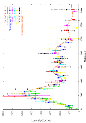
Figure 1: The CMB data used in this analysis: beam and calibration errors are not included.

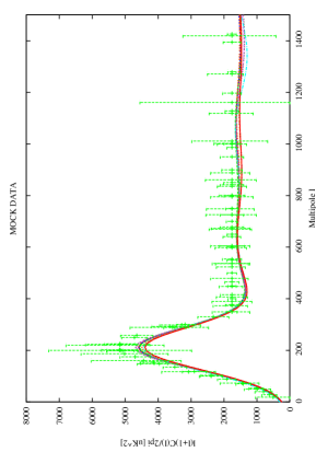
Figure 2: The 10 best MCMC samples fitting mock data. The data were generated by convolving the experimental window functions with a power spectrum consisting of a first peak followed by a flat line.

The phenomenological fit is operated through an MCMC algorithm. The MCMC approach is to generate a random walk through parameter space that converges towards the most likely value of the parameters and samples the parameter space following the posterior probability distribution. In the general case, the number of parameters and their priors have to be defined. There is no limit in resolution (except numerical precision of the computer). The priors define the volume in parameter space in which the random walk takes place.
At each iteration, a point $\mathbf{x}_{n+1}$ is randomly selected in the $m$-dimensional parameter space. Its likelihood is evaluated by comparing to the data. A sample is said to be accepted into the Markov chain or not, depending on the following acceptance criterion:

$$u\leq\min\left\{1,\frac{p(\mathbf{x}_{n+1})\mathcal{L}(\mathbf{x}_{n+1})}{p(\mathbf{x}_{n})\mathcal{L}(\mathbf{x}_{n})}\right\},$$

where $u$ is a random number sampled from a uniform distribution on the interval $[0,1]$, $p(\mathbf{x})$ is the prior and $\mathcal{L}(\mathbf{x})$ is the likelihood, containing the information from the data. At the end of the MCMC routine, the samples are counted and their number density projected onto one or more dimensions is proportional to the marginalised posterior distribution of the parameters. If the posterior follows a gaussian distribution, the best fit value is obtained by averaging over the samples. The MCMC procedure is described in more detail in saralewis and christensen .

We use wide uniform priors for each parameter, in which our resulting likelihoods are fully encompassed, except for the widths of the secondary gaussians which are not well constrained by the data. We run the MCMC routine in order to get $\sim 7000$ samples for each subset of data. Also, in order to check that out parametrisation is not biased towards the presence of peaks, we test it to fit a flat spectrum. We generate a set of mock data by convolving a power spectrum consisting of a peak and a flat line with the experimental window functions. The results show that a flat power spectrum is easily recovered within our priors, as shown in figure 2.

We then consider a flat, adiabatic, $\Lambda$-CDM model template of CMB angular power spectra, computed with CMBFAST (sz ), sampling the various parameters as follows: $\Omega_{cdm}h^{2}\equiv\omega_{cdm}=0.01,...0.40$, in steps of $0.01$; $\Omega_{b}h^{2}\equiv\omega_{b}=0.001,...,0.040$, in steps of $0.001$ and $\Omega_{\Lambda}=0.0,...,0.95$, in steps of $0.05$. The value of the Hubble constant is not an independent parameter, since:

$$h=\sqrt{{\omega_{cdm}+\omega_{b}}\over{1-\Omega_{\Lambda}}}.$$ (3)

We vary the spectral index of the primordial density perturbations within the range $n_{s}=0.60,...,1.40$ (in steps of $0.02$).

For each model in the template we then consider the corresponding values $\Delta T_{i}$, $\ell_{i}$, $\sigma_{i}$ such that the formula in Eq. (1) represents the best fit to its shape. Indeed, the $\Delta T_{i}$ do not exactly correspond to the amplitudes of the peaks, as our spectrum is a sum of gaussians and the power from each gaussian contribute over the whole spectrum. We find that, restricting the range in $\ell$ to $50,...,1500$, equation (1) approximates the shape of the spectra in our template well (better than $\sim 10\%$ in $C_{\ell}$).

We also check that the use of different phenomenological functions such as lorentzians or log-normals has no relevant effect on our results.

It is important to note that we restrict the parametrisation of our template of theoretical models to a set of only $4$ parameters. However, because of the ’cosmic degeneracy’ in the CMB observables, this is enough to describe the possible shapes of the CMB spectra in the $\Lambda$-CDM scenario. Increasing the optical depth $\tau_{c}$ or adding a background of gravity waves, for example, is nearly equivalent to changing some of the parameters already considered like $n_{S}$ and $\omega_{b}$. On the other hand we characterize the peaks in the spectrum with a phenomenological fit based on $15$ parameters, which allows independent positions, amplitudes and widths of the observed features.

The comparison between the model-independent values $\Delta T_{i}$, $\ell_{i}$ and $\sigma_{i}$ obtained by fitting the data with Eq. (1) and the corresponding values expected in the template of theoretical models represents therefore a strong check of the theory and can give hints for the presence of systematics and/or new physics.

III Results

In Table 2 we report the $68\%$ limits on $\Delta T_{i}$, $\ell_{i}$ and $\sigma_{i}$ of Eq. 1 obtained by analyzing the present CMB data with an MCMC procedure for each subset of CMB data. We also report the constraints on combinations of those parameters that are more directly connected to the cosmological parameters (see the discussion below).

In Table 3 we report the correlation matrix between the parameters of our phenomenological fit. As we can see, important correlations exist between the parameters: for example, the amplitude of the peaks is highly anti-correlated with the widht of the adiacent gaussians. This further illustrate the utility of analyzing the data with a single fitting function in order to properly evaluate the statistical significance of the oscillations.

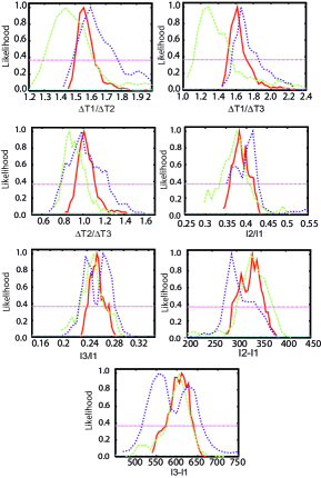
Figure 3: Marginalised likelihood functions for CMB observables. The red (solid), green (dashed) and blue (dotted) curves correspond to the following three data sets, respectively: Full data set, LF, HF.

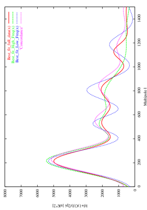
Figure 4: Comparison of the concordance cosmological power spectrum and the best-fit phenomenological power spectrum for each data subset.).

Figure 3 shows the marginalised likelihood functions of the important CMB observables, and the agreement between the three data subsets. Figure 4 shows the best-fit cosmological and phenomenological models. Although our sums of gaussians comprises any cosmological power spectrum to within $10\%$, their preferred shape differs from the cosmological model owing to the large parameter space allowing to fit the data very well.

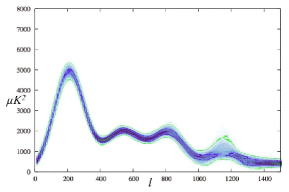
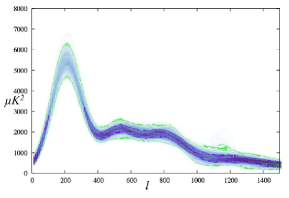
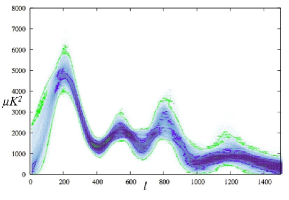
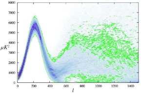
Figure 5: $68\%$ and $95\%$ confidence levels in the $\Delta T^{2}$, $\ell$ plane. The first three panels correspond to the full data set, HF data and LF data, respectively. The last panel shows the same result obtained by analysing the old data only. It is found to be consistent with the more recent data, and provides no constraints above $\ell\sim 400$ where the data provide no measurements. This shows where the power is well constrained by the data using our phenomenological function. Where no limits of power are found within $68\%$, it means that the data are not sufficient to constrain the power at that angular scale.

Figure 5 shows $68\%$ and $95\%$ confidence levels in power in the $\ell$-$\Delta T^{2}$ plane. This shows the most likely path of the power spectrum. These figures are generated as follows: First, we remind the reader that the number density of MCMC samples is proportional to the marginalised posterior. We divide the $\ell$-$\Delta T^{2}$ plane into pixels of size $10\times 10$. For each pixel, we count the phenomenological spectra that go through it. Hence, this is a density plot of our MCMC samples. The absence of a $68\%$ region at certain $\ell$ ranges indicates that more data are needed to constrain the power.

From figure 5, it appears that LF experiments provide constraints at high multipoles better than HF experiments which constrain the power at intermediate scales strongly. HF experiments also provide tight constraints at low $\ell$, mainly due to Archeops.

We also show the same result obtained by using the old data only. We find that the analysis provides no constraints above $\ell\sim 400$, as expected from the data. It is also consistent with the Archeops observations. Hence, when combining the old data with the LF data, HF data or both, our results remain essentially the same.

The values are in reasonable agreement with the results obtained by similar analyses (see e.g. debe2001 , boghdan , douspis , cbit ) and point towards the presence of multiple peaks in the spectrum.

The low frequency and high frequency experiments yield consistent results, showing that possible systematics due to galactic foregrounds are under control. However it is worth noticing that the LF data are more consistent with higher amplitude of secondary peaks. These experiments also use different techniques. The HF experiments are bolometers whereas the LF experiments are interferometers. The different nature of experimental uncertainties as well as their evaluation might suffer from different weaknesses contributing to enhance this contrast.

The CBI and ACBAR data at high $\ell$ are in agreement with the expected damping tail (see e.g. tail ). However, the poor spectral resolution ($\Delta{\ell}\sim 200$) does not allow us to constrain subsequent peaks.

Still, it is interesting to compare the values obtained with those expected in the $\Lambda$-CDM scenario with different priors, as we do in the last three columns of Table 2 (see caption).

Generally speaking, considering that the reported errors are at $1$-$\sigma$ and that the theoretical models are COBE normalized, which allows a further $10\%$ shift in amplitude, the model-independent values are in very good agreement with those predicted by the $\Lambda$-CDM models. It is interesting to notice that for the full data set, the subsequent peaks appear to be slightly lower in amplitude than those expected in the concordance model with $n_{S}=1$. This favors a spectral index $n_{S}$ slightly lower than one. However, there is a strong degeneracy between $n_{S}$ and the optical depth $\tau_{c}$ (see e.g. stompor ) and models with $n_{s}=1$ can be put in better agreement with the observations when increasing $\tau_{c}$.

Table 2: First 3 columns: 1-$\sigma$ constraints on the parameters of the phenomenological model for three subsets of data: The full data set, LF data and HF data. The allowed range for the same parameters in a database of COBE normalized theoretical models (no experimental data are considered) is also reported in the following $2$ columns for the case of weak priors ($0.05<\Omega_{cdm}<0.5$, $0.15<\Omega_{b}h^{2}<0.25$, $0.55<h<0.88$, $0.80<n_{S}<1.10$) and strong priors ($0.10<\Omega_{cdm}<0.35$, $0.18<\Omega_{b}h^{2}<0.22$, $0.65<h<0.80$, $0.95<n_{S}<1.05$). In the last column we also show the values for a COBE normalized concordance model with $\Omega_{cdm}=0.31$, $\Omega_{b}=0.04$, $h=0.7$ and $n_{s}=1$.

CMB	Full data set	High Frequency	Low Frequency	$\Lambda$-CDM	$\Lambda$-CDM	Concordance
Observable		Experiments	Experiments
	Phen. Fit	Phen. Fit	Phen. Fit	Weak Priors	Strong Priors
$\Delta T_{1}$	$69.3_{-2.3}^{+2.4}\mu K$	$70.7_{-3.5}^{+4.8}\mu K$	$68.9_{-4.1}^{+5.5}\mu K$	$(48-110)\mu K$	$(65-95)\mu K$	$74.9\mu K$
$\Delta T_{2}$	$44.0_{-1.9}^{+1.7}\mu K$	$43.1_{-3.0}^{+3.6}\mu K$	$46.8_{-4.3}^{+3.6}\mu K$	$(32-76)\mu K$	$(46-66)\mu K$	$53.6\mu K$
$\Delta T_{3}$	$43.8_{-4.4}^{+2.1}\mu K$	$40.7_{-5.0}^{+4.3}\mu K$	$54.4_{-11.2}^{+3.4}\mu K$	$(36-67)\mu K$	$(49-60)\mu K$	$54.6\mu K$
$\Delta T_{4}$	$31.2_{-8.7}^{+5.7}\mu K$	$25.7_{-5.7}^{+3.1}\mu K$	$27.9_{-7.3}^{+8.7}\mu K$	$(22-40)\mu K$	$(26-37)\mu K$	$35.6\mu K$
$\Delta T_{5}$	$19.8_{-3.8}^{+1.8}\mu K$	$18.4_{-5.2}^{+3.2}\mu K$	$20.6_{-17.3}^{+12.7}\mu K$	$(19-36)\mu K$	$(22-32)\mu K$	$27.6\mu K$
$\ell_{1}$	$208.8_{-6.1}^{+6.2}$	$204.6_{-7.9}^{+11.4}$	$206.8_{-22.0}^{+10.8}$	$192-279$	$203-242$	$215$
$\ell_{2}$	$550_{-45}^{+13}$	$505_{-21}^{+25}$	$533_{-20}^{+25}$	$464-696$	$488-594$	$514$
$\ell_{3}$	$824_{-41}^{+12}$	$764_{-42}^{+74}$	$806_{-36}^{+26}$	$692-1086$	$732-919$	$781$
$\ell_{4}$	$1145_{-45}^{+30}$	$1158_{-67}^{+242}$	$1189_{-87}^{+32}$	$1140-1386$	$1210-1301$	$1190$
$\ell_{5}$	$1474_{-79}^{+153}$	$1649_{-262}^{+142}$	$1515_{-346}^{+81}$	$1380-1590$	$1460-1550$	$1491$
$\sigma_{1}$	$93.3_{-5.2}^{+4.5}$	$90.3_{-6.2}^{+8.2}$	$88.2_{-12.3}^{+12.7}$	$86-136$	$86-108$	$93$
$\sigma_{2}$	$111.2_{\mbox{\tiny unbounded}}^{+27.7}$	$78.2_{-12.2}^{+19.3}$	$61.9_{\mbox{\tiny unbounded}}^{+36.7}$	$71-121$	$71-107$	$86$
$\sigma_{3}$	$82.5_{-23.1}^{+20.7}$	$136.3_{\mbox{\tiny unbounded}}^{+94.2}$	$69.8_{\mbox{\tiny unbounded}}^{+12.8}$	$86-150$	$86-150$	$102$
$\sigma_{4}$	not constrained	not constrained	not constrained	$70-120$	$70-110$	$87$
$\sigma_{5}$	not constrained	not constrained	not constrained	$70-120$	$75-110$	$88$
$\ell_{1}/\ell_{2}$	$0.382_{-0.024}^{+0.033}$	$0.415_{\mbox{\tiny unbounded}}^{+0.014}$	$0.376_{-0.042}^{+0.021}$	$0.379-0.429$	$0.402-0.422$	$0.418$
$\ell_{1}/\ell_{3}$	$0.256_{-0.016}^{+0.010}$	$0.266_{-0.040}^{+0.012}$	$0.251_{-0.013}^{+0.012}$	$0.242-0.290$	$0.259-0.281$	$0.275$
$\Delta T_{1}/\Delta T_{2}$	$1.56_{-0.07}^{+0.04}$	$1.60_{-0.12}^{+0.17}$	$1.44_{-0.15}^{+0.15}$	$1.23-1.68$	$1.32-1.51$	$1.40$
$\Delta T_{1}/\Delta T_{3}$	$1.62_{-0.11}^{+0.06}$	$1.65_{-0.10}^{+0.15}$	$1.29_{-0.18}^{+0.22}$	$1.12-2.13$	$1.26-1.73$	1.37
$\Delta T_{2}/\Delta T_{3}$	$1.01_{-0.09}^{+0.10}$	$0.99_{-0.12}^{+0.20}$	$0.87_{-0.10}^{+0.13}$	$0.80-1.32$	$0.92-1.17$	$0.98$
$\ell_{2}-\ell_{1}$	$332_{-42}^{+19}$	$290_{-19}^{+39}$	$329_{-30}^{+47}$	$267-427$	$284-353$	$299$
$\ell_{3}-\ell_{1}$	$611_{-39}^{+26}$	$555_{-41}^{+97}$	$605_{-30}^{+31}$	$484-817$	$528-679$	$566$

Table 3: Correlation matrix for the $15$ phenomenological parameters when fitted to the full data set.

	$\Delta T_{1}$	$\Delta T_{2}$	$\Delta T_{3}$	$\Delta T_{4}$	$\Delta T_{5}$	$\ell_{1}$	$\ell_{2}$	$\ell_{3}$	$\ell_{4}$	$\ell_{5}$	$\sigma_{1}$	$\sigma_{2}$	$\sigma_{3}$	$\sigma_{4}$	$\sigma_{5}$
$\Delta T_{1}$	$1.00$	$0.20$	$0.32$	$0.12$	$0.06$	$-0.02$	$-0.17$	$-0.07$	$0.03$	$-0.02$	$-0.23$	$-0.19$	$0.12$	$-0.18$	$0.04$
$\Delta T_{2}$	$0.20$	$1.00$	$0.03$	$-0.06$	$-0.07$	$-0.30$	$0.54$	$0.54$	$-0.15$	$0.00$	$-0.32$	$0.38$	$-0.70$	$0.18$	$0.11$
$\Delta T_{3}$	$0.32$	$0.03$	$1.00$	$0.37$	$0.07$	$0.38$	$-0.54$	$-0.27$	$0.40$	$0.08$	$0.30$	$-0.63$	$0.40$	$-0.45$	$-0.08$
$\Delta T_{4}$	$0.12$	$-0.06$	$0.37$	$1.00$	$0.32$	$0.06$	$-0.19$	$0.08$	$0.20$	$-0.10$	$0.03$	$-0.13$	$0.27$	$-0.71$	$-0.10$
$\Delta T_{5}$	$0.06$	$-0.07$	$0.07$	$0.32$	$1.00$	$-0.03$	$0.01$	$0.16$	$-0.36$	$-0.61$	$-0.07$	$0.05$	$0.06$	$-0.51$	$-0.09$
$\ell_{1}$	$-0.02$	$-0.30$	$0.38$	$0.06$	$-0.03$	$1.00$	$-0.42$	$-0.55$	$0.10$	$0.08$	$0.60$	$-0.75$	$0.49$	$-0.09$	$-0.05$
$\ell_{2}$	$-0.17$	$0.54$	$-0.54$	$-0.19$	$0.01$	$-0.42$	$1.00$	$0.72$	$-0.37$	$-0.09$	$-0.32$	$0.79$	$-0.84$	$0.31$	$0.08$
$\ell_{3}$	$-0.07$	$0.54$	$-0.27$	$0.08$	$0.16$	$-0.55$	$0.72$	$1.00$	$-0.04$	$-0.13$	$-0.52$	$0.77$	$-0.58$	$-0.07$	$0.01$
$\ell_{4}$	$0.03$	$-0.15$	$0.40$	$0.20$	$-0.36$	$0.10$	$-0.37$	$-0.04$	$1.00$	$0.64$	$0.10$	$-0.23$	$0.48$	$-0.20$	$-0.25$
$\ell_{5}$	$-0.02$	$0.00$	$0.08$	$-0.10$	$-0.61$	$0.08$	$-0.09$	$-0.13$	$0.64$	$1.00$	$0.11$	$-0.09$	$0.10$	$0.34$	$-0.19$
$\sigma_{1}$	$-0.23$	$-0.32$	$0.30$	$0.03$	$-0.07$	$0.60$	$-0.32$	$-0.52$	$0.10$	$0.11$	$1.00$	$-0.66$	$0.42$	$-0.01$	$-0.06$
$\sigma_{2}$	$-0.19$	$0.38$	$-0.63$	$-0.13$	$0.05$	$-0.75$	$0.79$	$0.77$	$-0.23$	$-0.09$	$-0.66$	$1.00$	$-0.74$	$0.20$	$0.05$
$\sigma_{3}$	$0.12$	$-0.70$	$0.40$	$0.27$	$0.06$	$0.49$	$-0.84$	$-0.58$	$0.48$	$0.10$	$0.42$	$-0.74$	$1.00$	$-0.46$	$-0.09$
$\sigma_{4}$	$-0.18$	$0.18$	$-0.45$	$-0.71$	$-0.51$	$-0.09$	$0.31$	$-0.07$	$-0.20$	$0.34$	$-0.01$	$0.20$	$-0.46$	$1.00$	$-0.13$
$\sigma_{5}$	$0.04$	$0.11$	$-0.08$	$-0.10$	$-0.09$	$-0.05$	$0.08$	$0.01$	$-0.25$	$-0.19$	$-0.06$	$0.05$	$-0.09$	$-0.13$	$1.00$

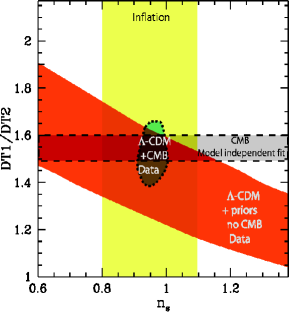
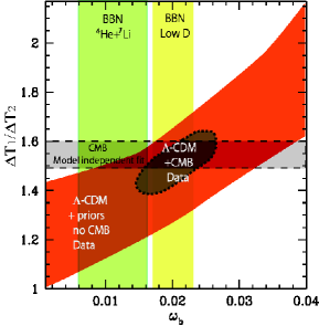
Figure 6: Observed relative amplitude between the first and second peak and comparison with adiabatic $\Lambda$-CDM cosmological models. The red region (“$\Lambda$-CDM no CMB”) defines all the values of $\Delta T_{1}/\Delta T_{2}$ present in the model template described in the text with the additional priors $0.1<\Omega_{cdm}<0.5$ and $0.55<h<0.88$. In the top panel, the additional prior $0.015<\Omega_{b}h^{2}<0.025$ is included, while in the bottom panel we use $0.8<n_{S}<1.1$. The $68\%$ c.l. constraint obtained by the phenomenological fit and he $95\%$ c.l. of all the $\Lambda-CDM$ models compatible with CMB are also plotted for comparison. The constraints on $\Omega_{b}h^{2}$ from standard BBN from $D$ (Burles et al.2001) and ${}^{4}He+^{7}Li$ (Cyburt et al. 2001) observations are also included in the second plot.

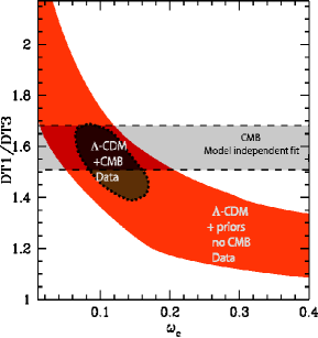
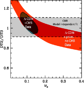
Figure 7: Observed relative amplitudes between the first and third peaks, and between the second and third peaks, and comparison with adiabatic $\Lambda$-CDM cosmological models. The red region (“$\Lambda$-CDM no CMB”) defines all the values of $\Delta T_{1}/\Delta T_{3}$ present in the template of models described in the text with the additional priors $0.55<h<0.88$, $0.015<\Omega_{b}h^{2}<0.025$ and $0.8<n_{S}<1.1$. The $68\%$ c.l. constraint obtained by the phenomenological fit and the $95\%$ c.l. of all the $\Lambda$-CDM models compatible with CMB are also plotted for comparison.

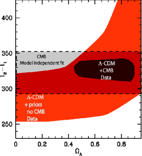
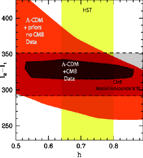
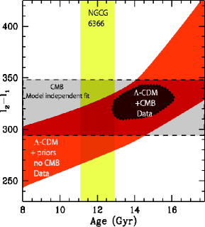
Figure 8: Observed relative positions between the first and second peak and comparison with adiabatic $\Lambda$-CDM cosmological models. The red region (“$\Lambda$-CDM no CMB”) defines all the values of $\ell_{2}-\ell_{1}$ present in the model template described in the text with the additional priors $0.015<\Omega_{b}h^{2}<0.025$ and $0.8<n_{S}<1.1$. In the top panel (constraints on $\Omega_{\Lambda}$) the additional prior $0.55<h<0.88$ is used. In the centre panel, we use $0.1<\Omega_{cdm}<0.5$. The band on the $y$-axis on the bottom panel is the constraint on the age of the oldest halo globular cluster in the sample of Salaris and Weiss ($1998$). The $68\%$ c.l. constraint obtained by the phenomenological fit and the $95\%$ c.l. of all the $\Lambda$-CDM models compatible with CMB are also plotted for comparison.

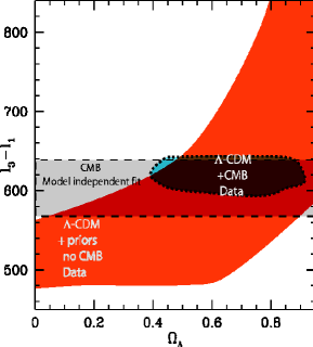
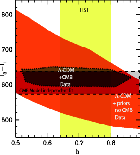
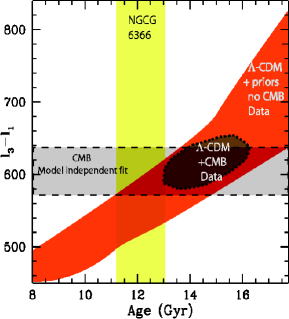
Figure 9: Observed relative positions between the first and third peak and comparison with adiabatic $\Lambda$-CDM cosmological models. The definitions of the regions and priors used are the same as in Fig. 8

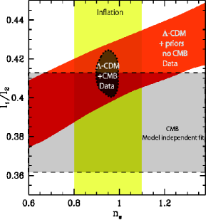
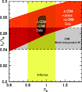
Figure 10: Observed relative positions between the first, second and third peak and comparison with adiabatic $\Lambda$-CDM cosmological models.The red region (“$\Lambda$-CDM no CMB”) defines all the values of $\ell_{1}/\ell_{2}$ and $\ell_{1}/\ell_{3}$ present in the modeltemplate described in the text with the additional priors $0.015<\Omega_{b}h^{2}<0.025$, $0.55<h<0.88$ and $0.1<\Omega_{cdm}<0.5$.The $68\%$ c.l. constraint obtained by the phenomenological fit and the $95\%$ c.l. of all the $\Lambda-CDM$ models compatible with CMB are also plotted for comparison.

We further investigate the consistency with $\Lambda$-CDM by considering phenomenological diagrams relating the relative amplitudes and positions of the peaks with variations in a specific physical parameter.

In the $\Lambda$-CDM adiabatic scenario, two key parameters control the relative power between the first and second peaks: the physical baryon density $\omega_{b}$ and the primordial spectral index $n_{S}$ (see e.g. bibbia ). Increasing $\omega_{b}$ enhances the odd-numbered peaks relative to the even-numbered ones, while increasing $n_{S}$ enhances the small-scale peaks relative to the ones at larger scales.

In figure 6 we plot the values allowed in our model template (restricted by a set of rather conservative cosmological constraints, see the caption) for the relative amplitude $\Delta T_{1}/\Delta T_{2}$ as functions of the parameters $\omega_{b}$ and $n_{S}$. As expected, increasing (decreasing) $\omega_{b}$ ($n_{S}$) increases $\Delta T_{1}/\Delta T_{2}$. The region is very broad, mainly owing to the degeneracy between these two parameters. Nevertheless, super-imposing the 1-$\sigma$ phenomenological constraint on $\Delta T_{1}/\Delta T_{2}$ in the diagram provides interesting constraints. Models with a value of the spectral index $n_{s}>1.15$, which are not easily accommodated in most inflationary models (see e.g. kinney and references therein) or in disagreement with the BBN constraint $\omega_{b}=0.020\pm 0.002$ are in fact not favored by our model-independent fit. In that figure, we also plot the constraints obtained by fitting the CMB data with the models in the template. This reduces in a severe way the number of allowed $\Lambda$-CDM models. Nevertheless, the result on relative amplitude of the peaks is completely consistent with the one derived by the phenomenological fit. This method provides better constraints on the amount of cold dark matter $\omega_{cdm}$ if we consider the relative amplitudes $\Delta T_{1}/\Delta T_{3}$ and $\Delta T_{2}/\Delta T_{3}$ as we do in the top and bottom panels of figure  7. A decrease in $\omega_{cdm}$ has the effect of decreasing the amplitude of the third peak (see e.g. gms ). As we can see, the two observational values of $\Delta T_{1}/\Delta T_{3}$ and $\Delta T_{2}/\Delta T_{3}$ provide similar constraints on $\omega_{cdm}$ in a non trivial way with $\omega_{cdm}\sim 0.12$ and with $\omega_{cdm}=0$ or $\omega_{cdm}>0.3$ in disagreement with the data.

In a flat $\Lambda$-CDM model a variation in $\Omega_{\Lambda}$ shifts the spectrum as $\ell\rightarrow{\cal R}\ell$ with the shift parameter ${\cal R}$ given by (see efsbond , melou ):

$${\cal R}=\sqrt{|\Omega_{m}|}\int_{0}^{z_{dec}}{[(1-\Omega_{\Lambda})(1+z)^{3}+\Omega_{\Lambda}]^{-1/2}dz}.$$ (4)

Varying the Hubble constant, parametrized as $H_{0}=100h$ Km/sec/Mpc, changes the scale of equality and produces a similar shift. These two parameters are related to the age of the universe by:

$$t_{0}=-9.8Gy\int_{\inf}^{0}{{{[h^{2}((1-\Omega_{\Lambda})(1+z)^{3}+\Omega_{\Lambda})]^{-1/2}}}dz}$$ (5)

We can therefore expect that a determination of the peak positions provides constraints on these three quantities.

In figure 8 and figure 9 we plot similar diagrams as above for $\ell_{2}-\ell_{1}$ and $\ell_{3}-\ell_{1}$ as functions of $\Omega_{\Lambda}$, $h$ and age, $t_{0}$. Even if the region of the allowed models is quite broad because of the intrinsic degeneracies, the observed peak positions strongly favor a model with cosmological constant $\Omega_{\Lambda}>0$, a Hubble parameter $h<0.8$, compatible with the Hubble Space Telescope (HST) result of $h=0.72\pm 0.08$ (freedman ), and an age $t_{0}>14$ Gy, compatible with the age of the oldest globular clusters (see e.g. age ). Again, the values obtained by the phenomenological fit are in agreement with those derived by the standard CMB+$\Lambda$-CDM analysis.

Another parameter that affects the position of the peaks is the spectral index $n_{S}$. However, the effect is different, the shift being scale dependent. Therefore, it is better to consider the quantities $\ell_{1}/\ell_{2}$ and $\ell_{1}/\ell_{3}$ which are unaffected by the overall shift $\cal R$. The corresponding diagrams are plotted in figure 10. As mentioned earlier, the observed values point towards a low value of the spectral index $n_{S}\leq 1$.

IV Conclusions

In this paper we investigated the consistency of the most recent CMB data with a class of $\Lambda$-CDM adiabatic inflationary models. First we characterized the positions, amplitudes and widths of the peaks by fitting the data with simple phenomenological functions composed by several gaussians. The detection of the peak amplitudes and positions is quite robust and stable between different data sets. We found that all the features are consistent with those expected by the standard theory. We also examined where the data contains the most information in the power-angular scale plane. We found that the low frequency experiments provide good constraints at small angular scales, consistent with the expected damping tail, whereas high frequency experiments provide strong limits on the power at large and intermediate scales. We observe that HF experiments and LF experiments yield very consistent results, although LF data seems to provide evidence for higher secondary oscillations. Overall, the power spectrum is now well determined until $\ell\sim 1500$. The inclusion of older data does not affect our conclusions as they do not measure the power beyond $\ell\sim 400$.

Furthermore, we related the features in the spectrum with several cosmological parameters by introducing cosmological diagrams that can be used for quick, by-eye, parameter estimations.

The relative amplitude of the first and second peak, in particular, of about $\sim 1.56$ is consistent with the baryon density expected from BBN and suggests a value of $n_{S}$ lower than one in the case of negligible reionization. The amplitudes of the third peak relative to the first and to the second, $\Delta T_{1}/\Delta T_{3}\sim 1.6$ and $\Delta T_{2}/\Delta T_{3}\sim 1$ strongly suggest the presence of cold dark matter but also limits time its contribution to values $\omega_{cdm}<0.2$. The relative positions of the peaks, $\ell_{2}-\ell_{1}\sim 330$ and $\ell_{3}-\ell_{1}\sim 610$ is pointing towards the presence of a cosmological constant, a Hubble parameter on the low side of the value allowed by the recent HST measurements ($h\sim 0.65$) and to an age of the universe $t_{0}\sim 14.5$ Gyrs consistent with the measurements of the oldest globular clusters.

It is reassuring that all those conclusions, obtained by just drawing few lines in the diagrams presented in Figs. $5-9$, are in agreement with the results obtained by a more careful standard analysis. Within the models considered in our database we found (at $68\%$ c.l.): $n_{s}=0.96\pm 0.03$, $\omega_{b}=0.022\pm 0.003$, $\omega_{cdm}=0.12\pm 0.03$, $\Omega_{\Lambda}=0.63\pm 0.16$, and $t_{0}=14.2\pm 0.7$ Gyrs.

The results obtained here show no need for modifications to the standard model, like gravity waves, quintessence, isocurvature modes, or extra-backgrounds of relativistic particles. Furthermore, possible systematic effects due to unknown foregrounds or calibration and beam uncertainties are not immediately suggested, since the different data sets are consistent with the theory.

Even if the width of the gaussians is poorly constrained, we found supporting evidence for multiple oscillations in the data between $430<\ell<910$. Beyond that, the newest experimental results show a damping of the power.

It is the duty of future satellite CMB experiments to point out discrepancies that might place the possibility of new physics in a more favorable light.

Acknowledgements It is a pleasure to thank Ruth Durrer, Anthony Lewis, Ruediger Kneissl, Roya Mohayaee, Lyman Page, Joseph Silk and Anze Slosar for useful comments. We acknowledge the use of CMBFAST sz . CJO is supported by the Leenaards Foundation, the Acube Fund, an Isaac Newton Studentship and a Girton College Scholarship. AM is supported by PPARC.

References

- (1)
- (2) E. Torbet et al., Astrophys. J. 521 (1999) L79 [arXiv:astro-ph/9905100]; A. D. Miller et al., Astrophys. J. 524 (1999) L1 [arXiv:astro-ph/9906421].
- (3) P. D. Mauskopf et al. [Boomerang Collaboration], Astrophys. J. 536 (2000) L59 [arXiv:astro-ph/9911444]; A. Melchiorri et al. [Boomerang Collaboration], Astrophys. J. 536 (2000) L63 [arXiv:astro-ph/9911445].
- (4) C. B. Netterfield et al. [Boomerang Collaboration], arXiv:astro-ph/0104460.
- (5) N. W. Halverson et al., arXiv:astro-ph/0104489.
- (6) A. T. Lee et al., Astrophys. J. 561 (2001) L1 [arXiv:astro-ph/0104459].
- (7) T. J. Pearson et al., astro-ph/0205388, (2002).
- (8) P. F. Scott et al., astro-ph/0205380, (2002).
- (9) A. Benoit [the Archeops Collaboration], arXiv:astro-ph/0210305.
- (10) C. l. Kuo et al.,
- (11) J. E. Ruhl et al., arXiv:astro-ph/0212229.
- (12) K. Grainge et al., arXiv:astro-ph/0212495.
- (13) W. Hu, N. Sugiyama and J. Silk, Nature 386, 37 (1997) [arXiv:astro-ph/9604166].
- (14) A. Kosowsky, M. Milosavljevic, R. Jimenez, astro-ph/0206014, (2002).
- (15) M.Kaplinghat, L. Knox, C. Skordis, astro-ph/0203413, (2002).
- (16) P. de Bernardis et al., [Boomerang Collaboration], arXiv:astro-ph/0105296.
- (17) C. Pryke, N. W. Halverson, E. M. Leitch, J. Kovac, J. E. Carlstrom, W. L. Holzapfel and M. Dragovan, arXiv:astro-ph/0104490.
- (18) R. Stompor et al., Astrophys. J. 561 (2001) L7 [arXiv:astro-ph/0105062].
- (19) A. Benoit [the Archeops Collaboration], arXiv:astro-ph/0210306.
- (20) A. Slosar et al., arXiv:astro-ph/0212497.
- (21) X. Wang, M. Tegmark, M. Zaldarriaga, astro-ph/0105091.
- (22) X. Wang, M. Tegmark, B. Jain and M. Zaldarriaga, arXiv:astro-ph/0212417.
- (23) J. L. Sievers et al., astro-ph/0205387, 2002.
- (24) J. A. Rubino-Martin et al., astro-ph/0205367, 2002.
- (25) R. Bean and A. Melchiorri, Phys. Rev. D 65 (2002) 041302 [arXiv:astro-ph/0110472]; A. Melchiorri, L. Mersini, C. J. Odman and M. Trodden, arXiv:astro-ph/0211522.
- (26) S. Burles, K. M. Nollett and M. S. Turner, Astrophys. J. 552, L1 (2001) [arXiv:astro-ph/0010171].
- (27) S. H. Hansen et al., Phys. Rev. D 65, 023511 (2002) [arXiv:astro-ph/0105385].
- (28) R. H. Cyburt, B. D. Fields and K. A. Olive, New Astron. 6 (1996) 215 [arXiv:astro-ph/0102179].
- (29) A. Melchiorri and J. Silk, arXiv:astro-ph/0203200.
- (30) M. Bucher, K. Moodley and N. Turok, Phys. Rev. Lett. 87, 191301 (2001) [arXiv:astro-ph/0012141].
- (31) L. Amendola, C. Gordon, D. Wands and M. Sasaki, Phys. Rev. Lett. 88 (2002) 211302 [arXiv:astro-ph/0107089].
- (32) R. Durrer, M. Kunz and A. Melchiorri, Phys. Rev. D 63 (2001) 081301 [arXiv:astro-ph/0010633].
- (33) F. R. Bouchet, P. Peter, A. Riazuelo and M. Sakellariadou, Phys. Rev. D 65, 021301 (2002) [arXiv:astro-ph/0005022].
- (34) R. Dave, R. R. Caldwell, P. J. Steinhardt, astro-ph/0206372, 2002.
- (35) S. Hannestad, S. H. Hansen and F. L. Villante, Astropart. Phys. 16, 137 (2001) [arXiv:astro-ph/0012009].
- (36) L. Covi and D. H. Lyth, arXiv:astro-ph/0008165; L. Covi, D. H. Lyth and A. Melchiorri, arXiv:hep-ph/0210395.
- (37) J. Magueijo, A. Albrecht, P. Ferreira and D. Coulson, Phys. Rev. D 54, 3727 (1996) [arXiv:astro-ph/9605047].
- (38) M. Tegmark, M. Zaldarriaga, astro-ph/0207047, (2002).
- (39) S. Hancock, G. Rocha, A. N. Lasenby & C. M. Guttierez, MNRAS, 294, L1, 1996 [arXiv:astro-ph/9612016].
- (40) L. Knox & L. Page, Phys.Rev.Lett. 85 (2000) 1366-1369.
- (41) A. Miller et al., arXiv:astro-ph/0108030.
- (42) R. Durrer, B. Novosyadlyj, S. Apunevych, astro-ph/0111594, (2001)
- (43) S. Podariu, T. Souradeep, J. R. Gott, B. Ratra and M. S. Vogeley, Astrophys. J. 559 (2001) 9 [arXiv:astro-ph/0102264].
- (44) S. L. Bridle, R. Crittenden, A. Melchiorri, M. P. Hobson, R. Kneissl and A. N. Lasenby, arXiv:astro-ph/0112114.
- (45) Seljak, U. & Zaldarriaga, M. 1996, Astrophys. J. , 469, 437.
- (46) A. Albrecht, D. Coulson, P. Ferreira and J. Magueijo, Phys. Rev. Lett. 76, 1413 (1996) [arXiv:astro-ph/9505030].
- (47) P. Binetruy and J. Silk, Phys. Rev. Lett. 87 (2001) 031102 [arXiv:astro-ph/0007452].
- (48) N. Aghanim, P. G. Castro, A. Melchiorri and J. Silk, arXiv:astro-ph/0203112.
- (49) G. Efstathiou, MNRAS, 332, 193 (2002) [arXiv:astro-ph/0109151].
- (50) A. Melchiorri and C. J. Odman, Phys. Rev. D 67, 021501 (2003) [arXiv:astro-ph/0210606].
- (51) A. Lewin and A. Albrecht, Phys. Rev. D 64, 023514 (2001) [arXiv:astro-ph/9908061].
- (52) R. Trotta, A. Riazuelo and R. Durrer, Phys. Rev. Lett. 87, 231301 (2001)[arXiv:astro-ph/0104017].
- (53) M. Douspis and P. G. Ferreira, Phys. Rev. D 65 (2002) 087302.
- (54) W. Hu, M. Fukugita, M. Zaldarriaga and M. Tegmark, Astrophys. J. 549 (2001) 669 [arXiv:astro-ph/0006436].
- (55) A. Lewis and S. Bridle, arXiv:astro-ph/0205436.
- (56) N. Christensen & R. Meyer, astro-ph/0006401, 2000.
- (57) W. H. Kinney, A. Melchiorri and A. Riotto, Phys. Rev. D 63 (2001) 023505 [arXiv:astro-ph/0007375].
- (58) L. M. Griffiths, A. Melchiorri and J. Silk, Astrophys. J. 553 (2001) L5 [arXiv:astro-ph/0101413].
- (59) G. Efstathiou & J.R. Bond [astro-ph/9807103].
- (60) W. Freedman, et al., Astrophysical Journal, 553, 2001, 47.
- (61) Salaris, M. & Weiss A., A & A, 1998, 335, 943.
- (62) M. White, Astrophys.J. 555 (2001) 88-91.
- (63) A. Melchiorri and L. M. Griffiths, arXiv:astro-ph/0011147.
- (64) Y. Xu, M. Tegmark and A. de Oliveira-Costa Phys. Rev. D 65 (2002) 083002
- (65) Wilson et al, et al., astro-ph/9902047.
- (66) P. Mauskopf et al, Astrophys. J. Letters 536 (2000) L59
- (67) K. Coble et al, astro-ph/0206254.