Topological changes of the photospheric magnetic field inside active regions: a prelude to flares

L. Sorriso-Valvo^1,2, V. Carbone¹, V. Abramenko³, V. Yurchyshyn^3,4, A. Noullez², H. Politano², A. Pouquet⁵, P. Veltri¹

Abstract

The observations of magnetic field variations as a signature of flaring activity is one of the main goal in solar physics. Some efforts in the past give apparently no unambiguous observations of changes. We observed that the scaling laws of the current helicity inside a given flaring active region change clearly and abruptly in correspondence with the eruption of big flares at the top of that active region. Comparison with numerical simulations of MHD equations, indicates that the change of scaling behavior in the current helicity, seems to be associated to a topological reorganization of the footpoint of the magnetic field loop, namely to dissipation of small scales structures in turbulence. It is evident that the possibility of forecasting in real time high energy flares, even if partially, has a wide practical interest to prevent the effects of big flares on Earth and its environment.

Solar flares are sudden, transient energy release above active regions of the Sun (Priest, 1982). As a consequence of random motion of the footpoints of the magnetic field in the photospheric convection (Parker, 1988), flares represent the dissipation at the many tangential discontinuities arising spontaneously in the magnetic fields of active regions. The magnetic energy is released in various form as thermal, soft and hard X-ray, accelerated particles etc. The observations of magnetic field variations, as a signature of flares above active regions, has been one of the main goals in solar physics, and some attempts for this has been made in the past (e.g. Hagyard et al., 1999 and references therein). All efforts give apparently no unambiguous observations of changes. This is due to the fact that often investigations try to look for changes of the vector magnetic field as a whole. Recently, unambiguous observations of changing have been reported by Yurchyshyn et al., 2000. The authors observed some typical changes of the scaling behavior of the current helicity calculated inside an active region of the photosphere, connected to the eruption of big flares above that active region. In the present paper we conjecture that the changes in the scaling behavior of the observed quantity is related to the occurrence of changes in the topology of the magnetic field at the footpoint of the loop.

The occurrence of scaling of signed measures calculated from scalar fields $f(\mbox{\boldmath$x$})$ which oscillate in sign can be studied through the following steps. First of all, introduce the signed measure

\mu_{i}(r)=\int_{Q_{i}(r)}f(\mbox{\boldmath$x$})d\mbox{\boldmath$x$}

(1)

through a coarse-graining of non overlapping boxes $Q_{i}(r)$ of size $r$ , covering the whole field defined on a region of size $L$ . It has been observed (Ott et al., 1992) that, for fields presenting self-similarity, this quantity displays well defined scaling laws. That is, in a range of scales $r$ , the partition function $\chi(r)$ , defined as

\chi(r)=\sum_{Q_{i}(r)}|\mu_{i}(r)|\sim r^{-\kappa}

(2)

where the sum is extended over all boxes occurring at a given scale $r$ , follows a power-law behavior

\chi(r)\sim r^{-\kappa}\,.

(3)

The scaling exponent $\kappa$ has been called cancellation exponent (Ott et al., 1992) because it represents a quantitative measure of the scaling behavior of imbalance between negative and positive contributions in the measure. For a positive definite measure or a smooth field $\kappa=0$ , while $\kappa=d/2$ for a completely stochastic field in a d-dimensional space (for example a field of uncorrelated points with $f=\pm 1$ , the sign being choosen randomly and independently for each point, with probability $1/2$ ). As the cancellations between negative and positive part of the measure decreases toward smaller scales, we get $\kappa>0$ , and this is the interesting situation. It is clear that the presence of structures in the field has an important effect on the cancellation exponent. For example, values of $\kappa<d/2$ , where $d$ is the dimension of the space (in the present paper $d=2$ ), indicate the presence of sign-persistent (i. e. smooth) structures.

Within turbulent flows, the value of the cancellation exponent can be related to the characteristic fractal dimension $D$ of turbulent structures on all scales using a simple geometrical argument (Sorriso-Valvo et al., 2002). Let $\lambda$ be the typical correlation length of that structures, of the order of the Taylor microscale (see for example Frisch, 1995), so that the field is smooth (correlated) in $D$ dimensions with a cutoff scale $\lambda$ , and uncorrelated in the remaining $d-D$ dimensions. If the field is homogeneous, the partition function (2) can be computed as $(L/r)^{d}$ times the integral over a generic box $Q(r)$ of size $r$ . The scaling of the latter can be estimated integrating over regular domains of size $\lambda^{d}$ and considering separately the number of contributions coming from the correlated dimensions of the field and those from the uncorrelated ones. The integration of the field over the smooth dimensions will bring a contribution proportional to their area $(r/\lambda)^{D}$ , while the uncorrelated dimensions will contribute as the integral of an uncorrelated field, that is proportional to the square root of their area $(r/\lambda)^{(d-D)/2}$ . Thus, when homogeneity is assumed, collecting all the contributions in (2) leads to scaling $\chi(r)\sim r^{-(d-D)/2}$ for the partition function, so that one can recover the simple relation

\kappa=(d-D)/2\;.

(4)

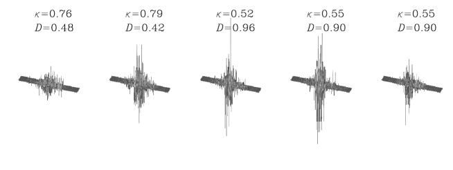
To get a quantitative measure of the change of the scaling of current helicity inside active regions, we used observations of the vector magnetic field obtained with the Solar Magnetic Field Telescope of the Beijing Astronomical Observatory (China). Measurements were recorded in the FeI 5324.19 Å spectral line. The field of view is about $218"\times 314"$ , corresponding to $512\times 512$ pixels on CCD. The magnetic field vector at the photosphere has been obtained through the measurements of the four Stokes parameters, and the current density $J_{z}(x,y)$ has been calculated as a line integral of the transverse field vector over a closed contour of dimension $1.72"\times 1.86"$ (cf. Yurchischin et al., 2000, for details). The current helicity $H_{c}={\bf B}\cdot{\bf J}$ (where ${\bf B}$ represents the magnetic field and ${\bf J}={\bf\nabla}\times{\bf B}$ the current density) is a measure of small scales activity in magnetic turbulence. It indicates the degree of clockwise or anti-clockwise knotness of the current density. Let us consider a magnetogram of size $L$ taken on the solar photosphere of an active region, and let ${\bf B}_{\perp}(x,y)$ the observed magnetic field perpendicular to the line of sight ( $(x,y)$ are the coordinate on the surface of the sun). Through this field we can measure the surrogate of current helicity, that is $h_{c}(x,y)=B_{z}(x,y)J_{z}(x,y)$ being $J_{z}(x,y)=[{\bf\nabla}\times{\bf B}_{\perp}]\cdot\mbox{\boldmath$\hat{e}_{z}$}$ . Figure 1^†^†margin: Figure 1 shows the current helicity surrogate of the active region NOAA 7590 for five different times, during the flaring event. The presence of signed structures is evident, as well as their evolution with time. A signed measure can be defined from this quantity

\mu_{i}(r)=\int_{Q_{i}(r)}h_{c}(x,y)dxdy\,.

(5)

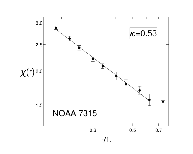
In figure 2^†^†margin: figure 2 we show, as example, the scaling behavior of $\chi(r)$ vs. $r$ for a flaring active region (NOAA 7315) which started to flare on October 22, 1992. At larger scales we find $\chi(r)\sim const.$ , and this is due to the complete balance between positive and negative contributions. The same behavior does not appear at smaller scales, showing that the resolution of the images is not high enough to resolve the smallest structures. In the intermediate region of scales, the cancellation exponent is found to be $\kappa=0.53\pm 0.09$ (Yurchischin et al., 2000).

Let us consider now what happens to the fractal dimension of current structures $D$ as a function of time. To this aim, we take different consecutive magnetograms of the same active region, and for each magnetogram, we compute the value of $\kappa$ and then of $D$ through relation (4). Note that, since cancellations in the vertical photospheric magnetic field $B_{z}(x,y)$ itself have been found to be very small (Lawrence et al., 1993; Abramenko et al., 1998), with a cancellation exponent of the order of $10^{-2}$ , cancellations of the current helicity are entirely due to the current structures.

In figure 3^†^†margin: figure 3 , we report the time evolution of $D$ superimposed to the flares occurred in two active regions, namely NOAAs 7315, and 7590 (which flared on October 1, 1993). Quite surprisingly we observe that the fractal dimension $D$ , starting from a given value ( $D<1$ ), becomes abruptly larger in correspondence with a sequence of big flares occurring at the top of the active region into the corona. The same behavior has been found for all calculations in all active regions we examined. The increase of the dimension of the structures may be the signature that dissipation has occured. In fact, annihilation is responsible for the smoothing of the small scales structures.

As shown in figure 2, a saturation of $\chi(r)$ is observed at large scales. At the smallest scales, the density of the measure must becomes smooth (no changes in sign are present) and we might thus found a saturation of $\chi(r)$ . The fact that we do not find this saturation is an indirect evidence that elementary flux tubes are smaller than the instrumental resolution. The change towards larger $D$ is then probabily due to the occurrence of dissipation of smaller and smaller flux tubes, that is magnetic energy is suddenly transferred towards small scales. This is the occurrence of an energy cascade towards smaller scales.

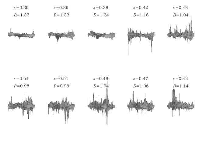
Using high resolution numerical simulation of two-dimensional ( $d=2$ ) turbulent magnetohydrodynamic flows (Politano et al., 1998; Sorriso-Valvo et al., 2000; Sorriso-Valvo et al., 2001), we can build up the signed measure for different fields. For example, since the geometry of the magnetic field $\mbox{\boldmath$B$}(x,y)=(B_{x},B_{y},0)$ is two-dimensional, the current $\mbox{\boldmath$J$}(x,y)=\nabla\times\mbox{\boldmath$J$}=(0,0,J_{z})$ has only the $z$ component, perpendicular to the 2-d simulation box, i. e. the plane $(x,y)$ . In Figure 4^†^†margin: Figure 4 we display the current field $J(x,y)$ for the numerical data, using ten snapshots in the statistically steady state, from $t=168$ up to $t=336$ in non-linear times units, $\tau_{NL}$ . As can be seen, the presence of positive and negative structures is evident as in the case of the solar data. A clear evolution of the complexity of the field is present. The signed measure of the current can be then computed as usual:

\mu_{i}(r)=\int_{Q_{i}(r)}\,J_{z}(x,y)\,dx\,dy\,\,,

and the scaling properties of the time averaged partition function are reported in figure 5^†^†margin: figure 5 . The power-law scaling (3) is clearly visible in a range extending from the large scales (near the integral scale of the flow $\ell_{0}\sim 0.2L$ , $L=2\pi$ being the size of the simulation box) down to a correlation lenght $r^{\star}$ of the order of the Taylor microscale $\lambda\sim 0.02L$ of the flow (see for example Frish, 1995). In this region, we fit the partition function to obtain the cancellation exponent $\kappa=0.43\pm 0.06$ . A saturation of the partition function is observed at a scale $r_{S}$ which is found to be of the order of the dissipative scale of the flow. In fact, for scales smaller than $r_{S}$ the dissipation stops the structures formation cascade, so that cancellations are stopped too. The fractal dimension of the current structures has been computed using the relation (4), which gives $D\simeq 1$ , indicating current structures similar to filaments. The presence of filaments can be clearly observed by a direct inspection of the current field contour plot, confirming the reliability of the model (see Sorriso-Valvo et al., 2002).

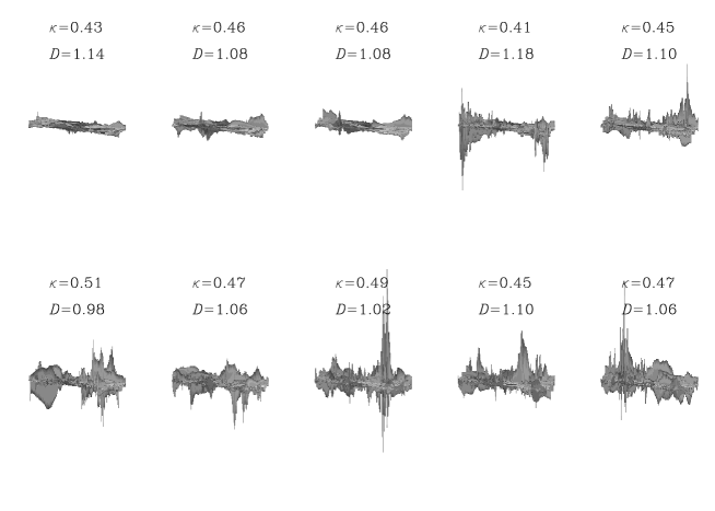
In order to compare more directely the numerical results with the solar data cancellation analisys, we introduce now a new surrogate for the current helicity. Since in two-dimensional geometry the current helicity is zero, the current being perpendicular to the magnetic field, we simply consider $H_{c}^{(2d)}(x,y)=J(x,y)|B(x,y)|$ , which is represented in Figure 6^†^†margin: Figure 6 for the same times snapshots as in Figure 4. The current helicity surrogate, as in the case of the solar data, appears smoother than the current itself, and keeps the same structures topology and evolution. The signed measure of such field is then computed as in the previous cases:

\mu_{i}(r)=\int_{Q_{i}(r)}\,H_{c}^{(2d)}(x,y)\,dx\,dy\,.

The scaling properties of the partition function $\chi(r)$ can be now represented by the cancellation exponent, obtained by the usual fitting procedure after time averaging. In Figure 7^†^†margin: Figure 7 we present the scaling of $\chi(r)$ , together with the fitting power-law, for which we find an exponent $\kappa=0.46\pm 0.03$ . This result is very close to the result obtained for the current, showing that for our numerical data as well, the current field is the one responsible for sign singularities, and its structures control the cancellations.

We want now to study in more detail the time evolution of the cancellations effects in the two-dimensional numerical simulations. To do this, we plot in Figure 8^†^†margin: Figure 8 the time evolution of the (kinetic) Reynolds number, together with the two cancellation exponents $\kappa_{j}$ and $\kappa_{H_{c}^{(2d)}}$ , for the snapshots already presented in Figures 4 and 6. As already pointed out, the first snapshots looks smoother than the others (see Figures 4 and 6, and this fact can be interpreted as stronger presence of dissipative effects for such times; correspondingly, the values of both the cancellation exponents are smaller, which means, following our model, that the fractal dimension of the structures $D$ is larger for these times. This observation confirm the results already obtained in Sorriso-Valvo et al, (2002) and discussed above. The Reynolds number also presents a time evolution, which is however shifted with respect to the evolution of the cancellation exponents. Unfortunately, due to the limited time interval of our simulations, it is impossible to say whether that shift is backward or foreward. Since the Reynolds number is related to the importance of dissipative effects against non linear effects in the turbulent cascade, it would be interesting to clarify this point as a further confirmation of our interpretation.

In this paper we point out that the changes in the scaling behavior of cancellations, measured through the cancellation exponent $\kappa$ , are due to the topology changes of the structures present in the field, and are thus related to the importance of dissipative effects. The non-linear turbulent cascade, underlying the formation os such structures on all scales, can be considered as one important input mechanism for flares. The results obtained from the analysis of the numerical simulations strongly support the interpretation of the observational results for the photospheric magnetic field in the active regions.

To conclude, it is evident that the behavior we found can be used as a signature of the occurrence of big flares. High energy solar flares become of great interest because they can produce severe damages on Earth. Power blackouts, break up of communications and mainly damage of satellites or space flights, can be ascribed to energy released during big solar flares. It is then evident that the possibility of forecasting, even if partially, high energy flares has a wide practical interest to prevent the effects of flares on Earth and its environment. We build up a model which allows us to recognize without ambiguity changing behavior of the photospheric magnetic field of active regions. These changes, pointed out through the variation of a scaling index for current helicity, can be seen mainly before the eruption of big flares. The change of scaling index is due to the turbulent and intermittent energy cascade towards smaller scales, a mechanism which could be identified as the input of flaring activity, where energy is dissipated. The method could allows us to forecast, in real time, the appearence of the strongest flaring activity above active regions.

References

Abramenko, V.I., Yurchyshyn V.B., and Carbone, V., Does the photospheric current take part in the flaring process?, Astron. Astrophys., 334, L57, 1998.

Boffetta, G., Carbone, V., Giuliani, P., Veltri, P., and Vulpiani, A., Power laws in solar flares: self-organized Criticality or Turbulence?, Phys. Rev. Lett., 83, 4662, 1999.

Hagyard, M.J., Stark, B.A., and Venkatakrishnan, P., A search for vector magnetic field variations associated with the M-class flares of 10 June 1991 in AR 6659, Sol. Phys., 184, 133, 1999.

Lawrence, J.K., Ruzmaikin, A.A., and Cadavid, A.C., Astrophys. J., 417, 805, 1993

Lepreti, F., Carbone, V., and Veltri, P., Solar flare waiting time distribution: varying-rate Poisson or Levy function?, Astrophys. J., 555, L133, 2001.

Ott, E., Du, Y., Sreenivasan, K.R., Juneja, A., and Suri, A.K., Phys. Rev. Lett., 69, 2654, 1992.

Politano, H., Pouquet, A., and Carbone, V., Determination of anomalous exponents of structure functions in two-dimensional magnetohydrodynamic turbulence, Europhys. Lett., 43, 516, 1998.

Priest, E., Solar Magnetohydrodynamic, D. Reidel Publishing Company, Dordrecht, 1982.

Sorriso-Valvo, L., Carbone, V., Noullez, A., Politano, H., Pouquet, A., and Veltri, P., Analysis of cancellation in two-dimensional MHD turbulence, Phys. Plasmas, 9, 89, 2002.

Sorriso-Valvo, L., Carbone, V., Veltri, P., Politano, H., and Pouquet, A., Non-gaussian probability distribution functions in two-dimensional magnetohydrodynamic turbulence, Europhys. Lett., 51, 520, 2000.

Yurchyshyn, V.B., Abramenko, V.I., and Carbone, V., Flare-related changes of an active region magnetic field, Astrophys. J., 538, 968, 2000.

Valentina I. Abramenko, Crimean Astrophysical Observatory, 98409 Nauchny, Crimea, Ukraine. (e-mail: avi@crao.crimea.ua) Vincenzo Carbone, Luca Sorriso-Valvo and Pierluigi Veltri, Dipartimento di Fisica and Istituto Nazionale di Fisica per la Materia, Ponte P. Bucci, Cubo 31C, Universitá della Calabria, I-87036 Rende (CS), Italy. (e-mail: carbone@fis.unical.it; sorriso@fis.unical.it; veltri@fis.unical.it) Alain Noullez and Helene Politano, Laboratoire Cassini, Observatoire de la Côte d’Azur, B. P. 4229, F-06304 Nice Cedex 04, France. (e-mail: anz@obs-nice.fr; politano@obs-nice,fr) Annick Pouquet, ASP/NCAR, P.O. Box 3000 Boulder, CO 80307-3000. (e-mail: pouquet@ucar.edu) V. Yurchyshyn, Big Bear Solar Observatory, 40386 North Shore Lane, Big Bear City, CA 92314-9672, U.S.A. (e-mail: vayur@bbso.njit.edu ) Received

¹Dipartimento di Fisica, Universitá della Calabria, and Istituto Nazionale di Fisica della Materia, sezione di Cosenza, Italy. ²Observatoire de la Côte d’Azur, Nice, France ³Crimean Astrophysical Observatory, Nauchny, Crimea, Ukraine ⁴Big Bear Solar Observatory, Big Bear City, CA ⁵ASP/NCAR, Boulder, CO

\@normalsize

Refer to caption — Figure 1.: The current helicity $H_{c}$ measured for the active region NOAA 7590. The five different plots are taken at different times, and include a $50$ hours interval. The presence of positive and negative strucutres on all scales is evidenced. The flat portion of field near the corners are due to removing in the projection effects. Over each plot the measured cancellation exponent $\kappa$ and the fractal dimension of structures $D$ are reported (see further for explaination).