Density profiles and clustering of dark halos and clusters of galaxies

Abstract

Density profiles of cosmological virialized systems, or dark halos, have recently attracted much attention. I first present a brief historical review of numerical simulations to quantify the halo density profiles. Then I describe the latest results on the universal density profile and their observational confrontation. Finally I discuss a clustering model of those halos with particular emphasis on the cosmological light-cone effect.

Department of Physics, The University of Tokyo, Tokyo 113-0033, Japan.

1. Introduction

The key assumption underlying the standard picture of structure formation is that the luminous objects form in a gravitational potential of dark matter halos. Therefore, a detailed description of halo density profiles as well as of their clustering properties is the most basic step toward constructing the formation and evolution of galaxies and clusters.

More specifically, the importance of the detailed studies of density profiles of dark halos is two-fold:

(i) theoretical interest;

What is the final (quasi-)equilibrium state of cosmological self-gravitating systems (as long as the energy dissipation is neglected) ? One may easily think of two quite distinct, but equally plausible, possibilities;

1. the systems reach a certain universal distribution which is independent of the cosmological initial condition.

2. the systems somehow keep the memory of the cosmological initial condition even at the highly nonlinear regime.

The singular isothermal sphere:

$$\rho(r)=\frac{\sigma^{2}}{2\pi G}\frac{1}{r^{2}}$$ (1)

may be a reasonable possibility along the line of the idea (A). As a matter of fact, quite often I meet people who argue that the idea (B) is unlikely because of the strong nonlinear nature of the gravitation. In such an occasion, I present an example of the well-known stable clustering solution for the nonlinear two-point correlation function (Davis & Peebles 1977):

$$P_{\rm mass}(k) \propto k^{n}\quad\rightarrow\quad\xi_{\rm mass}(r)\propto r^{-3(n+3)/(n+5)}.$$ (2)

This provides a good specific case that the cosmological initial condition is not erased and imprinted even in the strongly nonlinear behavior as is well confirmed by later numerical simulations (e.g., Suto 1993; Suginohara et al. 2001). Of course the answer to the final state of cosmological self-gravitating systems may not be unique since it should really depend on the specifics and scales of the systems under consideration. For instance, it is clearly hopeless to extract any meaningful cosmological information from the precise data on the orbit of the earth around the Sun; all the initial memory should have been lost due to the strongly nonlinear and chaotic nature of the gravitation. Nevertheless the final state of dark matter halos corresponding to galaxy- and cluster-scales is a well-defined problem which may be reliably answered with the current high-resolution numerical simulations independently of the physical intuition.

(ii) practical application;

Whether or not the density profiles of dark halos keep the cosmological initial memory, the quantitative (empirical) prediction of the profile for a given set of cosmological parameters has several profound astrophysical implications including the rotation curve of spiral galaxies, reconstruction of the mass distribution from the weak-lensing, and X-ray and SZ observations of galaxy clusters. In particular, the confrontation of those testable predictions against the accurate observational data may even challenge the cold dark matter paradigm itself.

In this article, first I will review the summary of the past studies of the density profiles of dark matter halos, and then present some applications of those results.

2. Previous work on the density profiles of dark matter halos

The study of the density profiles of cosmological self-gravitating systems or dark halos has a long history. Table 2 is my personal (and thus incomplete) summary of some past work that I recognize (or at least I have really read those papers).

Hoffman & Shaham (1985) argued, on the basis of the secondary infall model (Gunn & Gott 1972), that the density profile around peaks is given by $\rho\propto r^{-3(n+3)/(n+4)}$ where $n\equiv d\ln P(k)/d\ln k$ is the spectral index of the density fluctuation field. The resulting power index $-3(n+3)/(n+4)$ is close to, but slightly differ from, that for the stable clustering solution for the nonlinear two-point correlation function $-3(n+3)/(n+5)$. In any case this result implies that the density profile of dark halos does keep the initial memory.

Many subsequent numerical simulations seem to have confirmed the prediction of Hoffman & Shaham (1985). While some authors have reported the existence of a kind of universal profile, they were not able to specify its functional form. In this respect, the proposal of the specific universal density profile by Navarro, Frenk & White (1995, 1996, 1997) was really a breakthrough. They suggested that all simulated density profiles can be well fitted to the following simple model (now referred to as the NFW profile):

$$\rho(r)\propto{1\over(r/r_{\rm s})(1+r/r_{\rm s})^{2}}$$ (3)

by an appropriate choice of the scaling radius $r_{\rm s}=r_{\rm s}(M)$ as a function of the halo mass $M$. Considering the previous conclusion from numerical simulations, their claim was quite surprising and, in some sense, contradictory. It turned out that most simulations prior to their discovery did not have sufficient mass-resolution to reliably represent the deep central gravitational potential, which gives rise to an artificial central core. This presents a good example that the quantitative difference leads to the qualitatively different interpretation of the physical phenomena; now the density profile of dark halos seems to lose the initial memory, and thus the answer to the final (quasi-)equilibrium state of cosmological self-gravitating systems changes even in a qualitative way; from the possibility (A) to (B) mentioned in the previous section !

Table 1.: The stable solution and the density profile around peaks.

$n$	$\xi_{\rm stable}\propto r^{-3(n+3)/(n+5)}$	$\rho\propto r^{-3(n+3)/(n+4)}$
0	$r^{-1.8}$	$r^{-2.25}$
-1	$r^{-1.5}$	$r^{-2}$
-2	$r^{-1}$	$r^{-1.5}$

If this change of the qualitative conclusion (from Hoffman & Shaham to NFW) is really ascribed to the mass-resolution of the numerical simulations, one should naturally wonder whether or not current numerical simulations are sufficiently reliable for the present problem. This motivated many people to examine the convergence of the profile, in particular, its inner power-law index, with significantly higher–resolution simulations. Fukushige & Makino (1997) are the first to claim that the inner slope of density halos is much steeper than the NFW value. Their claim was confirmed by a series of systematic studies by Moore et al. (1998, 1999), and the current consensus among most (but not all) numerical simulators in this field is the converged profile is given by

$$\rho(r)\propto{1\over(r/r_{\rm s})^{\alpha}(1+r/r_{\rm s})^{3-\alpha}}$$ (4)

with $\alpha\approx 1.5$ rather than the NFW value, $\alpha=1$, (e.g., Fukushige & Makino 2001). In most cases this difference is fairly minor and the NFW profile still provides a good empirical approximation to the dark matter halo (Jing & Suto 2002).

I just reproduce two figures from my collaborative work (Jing & Suto 2000) just to illustrate the validity of the universal density profile (eq.[4]) despite the fact that their projected images look very diverse rather than universal. It is hard to imagine the regularity of the averaged profiles plotted in Figure 2 behind the apparent diversity quite visible in Figure 1.

Table 2.: Past work on the density profiles of dark matter halos.

1970	Peebles
	$N=300$ simulation to reproduce the profile of the Coma cluster
1977	Gunn
	predicted $\rho\propto r^{-9/4}$ on the basis of secondary infall model
1985	Hoffman & Shaham
	density profiles around the peak: $\rho\propto r^{-3(n+3)/(n+4)}$
1986	Quinn, Salmon & Zurek
	confirmed the Hoffman & Shaham prediction ($N\approx 1000$ simulation)
1987	West, Dekel & Oemler
	suggested of the existence of a kind of universal density profile
	with $N\approx 4000$ simulations.
1988	Frenk, White, Davis & Efstathiou
	reproduced the galactic rotation curve
	in the SCDM model with $N=32^{3}$ simulations
1990	Hernquist
	proposed an analytic model for density profiles of elliptical galaxies
	$\rho(r)=(Ma/2\pi)r^{-1}(r+a)^{-3}$
1994	Crone, Evrard, & Richstone
	suggested a central cusp (not a core) with $N=64^{3}$ simulations
1995	Navarro, Frenk & White
	discovered a universality in the halo density profile
	from SPH simulations in SCDM, $N\approx 6000$ per halo
	$\rho(r)=7500\bar{\rho}(r/0.2r_{200})^{-1}(1+r/0.2r_{200})^{-2}$
1996	Navarro, Frenk & White
	19 halos with $N(<r_{\rm vir})=5000-10000$ in SCDM
	suggested a specific form for the universal density profile
1997	Fukushige & Makino
	found a steeper inner profile with $N=786400$ simulations
1997	Navarro, Frenk & White
	universal density profile in a variety of cosmological models
1998	Syer & White
	repeated merger + tidal disruption model $\rightarrow$ $\rho\propto r^{-3(n+3)/(n+5)}$
1998	Moore et al.
	found a steeper inner profile $\rho\propto r^{-1.4}$
	consistent with the previous finding of Fukushige & Makino
1999	Moore et al.
	suggested that $\rho(r)\propto(r/r_{s})^{-1.5}[1+(r/r_{s})^{1.5}]^{-1}$
2000	Jing & Suto
	dependence of the inner slope on the halo mass (controvertial)
2002	Jing & Suto
	triaxial modeling of the universal dark matter density profiles

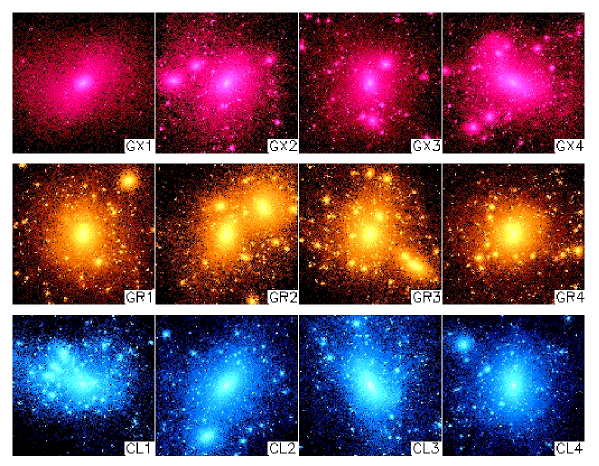
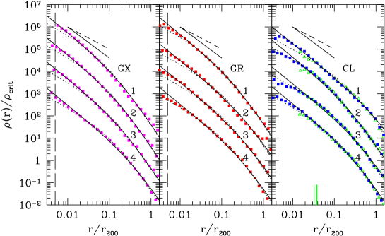
Figure 1.: Snapshots of the simulated halos at $z=0$. Top, center and bottom panels display the halos of galaxy, group and cluster masses (for four different realizations from left to right), respectively. The size of each panel corresponds to $2r_{\rm vir}$ of each halo (Jing & Suto 2000).

Figure 2.: Spherically-averaged radial density profiles of the simulated halos of galaxy (left), group (middle), and cluster (right) masses. The solid and dotted curves represent fits of $\alpha=1.5$ and $\alpha=1$ respectively. For reference, we also show $\rho(r)\propto r^{-1}$ and $r^{-1.5}$ in dashed and solid lines (Jing & Suto 2000).

3. Observational confrontation of the universal density profile

3.1. Mass profile and rotation curve

The advantage of the NFW profile is that it is completely specified for a given of cosmological parameters. Therefore this leads to a variety of testable quantitative predictions. In fact, one can write down all the necessary formulae in the following concise manner:

$$\rho_{\scriptscriptstyle\rm DM}(r) = \frac{\delta_{c}\rho_{\rm crit}}{(r/r_{\rm s})(1+r/r_{\rm s})^{2}},$$ (5)

where $\rho_{\rm crit}$(z) is the critical density of the universe at $z$

$$\rho_{\rm crit}(z)=\frac{3H_{0}^{2}(1+z)^{3}}{8\pi G}\approx 1.8\times 10^{11}(1+z)^{3}h^{2}M_{\odot}/{\rm Mpc}^{3}.$$ (6)

The characteristic halo density contrast $\delta_{c}$, and the scaling radius $r_{s}$ are written in terms of the concentration parameter as

$$\delta_{c} = \frac{\Delta_{\rm vir}\Omega_{0}}{3}\frac{c_{\rm vir}^{3}}{\ln(1+c_{\rm vir})-c_{\rm vir}/(1+c_{\rm vir})},$$ (7)

$$r_{s}(M) \equiv \frac{r_{\rm vir}(M)}{c_{\rm vir}}.$$ (8)

Finally the virial radius $r_{\rm vir}=r_{\rm vir}(M,z)$ and the concentration parameter are given as

$$r_{\rm vir}\equiv\left(\frac{3M}{4\pi\Delta_{\rm vir}\Omega_{0}\rho_{\rm crit}}\right)^{1/3}\approx\frac{1.69}{1+z}\left(\frac{\Delta_{\rm vir}\Omega_{0}}{18\pi^{2}}\right)^{-1/3}\left(\frac{M}{10^{15}h^{-1}M_{\odot}}\right)^{1/3},$$ (9)

$$\Delta_{\rm vir}\approx\left\{\begin{array}[]{ll}18\pi^{2}\Omega(z)^{-0.7}&\mbox{$(\lambda_{0}=0)$}\\ 18\pi^{2}\Omega(z)^{-0.6}&\mbox{$(\lambda_{0}=1-\Omega_{0})$}\end{array}\right.,$$ (12)

$$c_{\rm vir}(M,z)=\frac{9}{1+z}\left(\frac{M}{1.5\times 10^{13}h^{-1}M_{\odot}}\right)^{-0.13}.$$ (13)

The expression for $c_{\rm vir}$ is the fitting formula in LCDM (Lambda Cold Dark Matter) by Bullock et al. (2001).

Then the corresponding mass profile and the circular velocity are computed in a straightforward manner as

$$M(r)=4\pi\int_{0}^{r}\frac{\delta_{c}\rho_{\rm crit}r^{2}}{(r/r_{\rm s})(1+r/r_{\rm s})^{2}}dr=4\pi\delta_{c}\rho_{\rm crit}r_{s}^{3}\left[\ln\left(1+\frac{r}{r_{s}}\right)-\frac{r}{r+r_{s}}\right],$$ (14)

and

$$V_{c}(r)=\sqrt{\frac{GM(r)}{r}}=\sqrt{4\pi\delta_{c}\rho_{\rm crit}r_{s}^{2}\left[\frac{r_{s}}{r}\ln\left(1+\frac{r}{r_{s}}\right)-\frac{r_{s}}{r+r_{s}}\right]}.$$ (15)

The above results explicitly show that one can in principle compare the universal density profile with the observational data without any unknown free parameter. This is why the reported disagreement with the mass profile reconstructed from weak/strong lensing (Tyson et al. 1998) and the rotation curves of dwarf/low surface brightness galaxies (e.g., Moore et al. 1999; de Blok et al. 2001), if real, cannot be easily accommodated in the context of the standard paradigm of cold dark matter.

3.2. X-ray gas density profile from the universal density profile of dark halos: origin of the isothermal $\beta$ model ?

Another important application of the universal density profile of dark halos may be found in X-ray emission from galaxy clusters. A simple but realistic approximation is the isothermal gas distribution in hydrostatic equilibrium embedded in the NFW halo gravitational potential. Actually the hydrostatic equilibrium equation:

$$\frac{dp_{\rm gas}}{dr}=-\frac{GM(r)}{r^{2}}\rho_{\rm gas},$$ (16)

combined with the NFW profile and equation of state

$$p_{\rm gas}=n_{\rm gas}kT_{\rm gas}=\frac{\rho_{\rm gas}}{\mu m_{p}}kT_{\rm gas}$$ (17)

can be analytically integrated (Makino, Sasaki & Suto 1998; Suto, Sasaki & Makino 1998) as

$$\rho_{\rm gas}(r)=\rho_{\rm g0}~{}e^{-B}\left(1+\frac{r}{r_{s}}\right)^{Br_{s}/r},\qquad B\equiv\frac{G\mu m_{p}}{kT_{\rm gas}}4\pi\delta_{c}\rho_{\rm crit}r_{s}^{2}.$$ (18)

More surprising is the fact that the above model is very close to the conventional $\beta$ model. Indeed we found the following fit as illustrated in Figure 3:

$$\rho_{\rm gas}(r) \approx \frac{\rho_{g0}A}{[1+(r/r_{\rm c,eff})^{2}]^{3\beta_{\rm eff}/2}},$$ (19)

$$A \approx -0.178b+0.982=-0.013B+0.982~{}(b\equiv 2B/27),$$ (20)

$$r_{\rm c,eff} \approx 0.22r_{s},\qquad\beta_{\rm eff}\approx 0.9b=0.067B.$$

Figure 3.: Gas density profile (solid lines) expected from the universal density profile of dark matter halo (dashed line) for $b=1/3$, $1$, and $5/3$. For comparison, the best-fit $\beta$-models with $\beta=0.9b$ and $r_{c}=0.22r_{s}$ are plotted in dotted lines (Makino, Sasaki, & Suto 1998).

As far as I understand, this work is the first analytical model for the cluster gas distribution obtained by consistently solving the Poisson equation for the underlying halo mass distribution. The fact that the resulting gas profile is quite similar to the isothermal $\beta$ model, widely used as a good empirical model, is encouraging. On the other hand, the expected core sizes of clusters seem to be significantly smaller than the observational ones (Fig. 4). In fact, rotation curves of dwarf/LSB galaxies (Moore et al. 1999; de Blok et al. 2001) and the mass profile reconstructed for the galaxy cluster CL0024 (Tyson et al. 1998) also indicate the presence of the core, rather than cusp, in the halo density profile. While this is still controversial at this point, Spergel & Steinhard (2000) among others even proposed to abandon the collisionless nature of dark matter to reconcile the reported discrepancy.

Figure 4.: Predicted properties of gas density distribution as functions of the X-ray cluster gas temperature $T_{X}=T_{\rm vir}(r_{s})$. (a) Ratio of $r_{vir}$ and $r_{c}(\approx 0.22r_{s})$; (b) ratio of the virial temperatures at $r_{s}$ and at $r_{\rm vir}$; (c) predicted sizes of the effective core radius compared with the observed cluster data. Solid, dotted and dashed lines indicate SCDM, OCDM, and LCDM models, respectively.

3.3. Collisional dark matter

Since the cold dark matter model is known to successfully reproduce the large-scale structure of the universe ($r\gg 1$Mpc), the possible collision of dark matter should be effective only at scales below 1Mpc. The required collision cross section $\sigma$ for a dark matter particle of mass $m$ may be obtained by assuming

$$(mn)\left(\frac{\sigma}{m}\right)l\approx 1\quad{\rm for}~{}mn\approx\rho_{\rm c,cluster}~{}{\rm and}~{}l\approx 1{\rm Mpc}.$$ (21)

This may be rewritten as

$$\left(\frac{\sigma}{m}\right)\approx 1.6h^{-1}{\rm cm}^{2}/{\rm g}\left(\frac{10^{4}\rho_{\rm crit}}{\rho_{\rm c,cluster}}\right)\left(\frac{1h^{-1}{\rm Mpc}}{l}\right)$$ (22)

or equivalently as

$$\sigma\approx 2.5\times 10^{-24}h^{-1}{\rm cm}^{2}\left(\frac{m}{1{\rm GeV}}\right)\left(\frac{10^{4}\rho_{\rm crit}}{\rho_{\rm c,cluster}}\right)\left(\frac{1h^{-1}{\rm Mpc}}{l}\right).$$ (23)

The corresponding mean collision time-scale is

$$\Delta t\approx\frac{l}{v}\approx 10^{9}\left(\frac{1000{\rm km/s}}{v}\right)\left(\frac{l}{1h^{-1}{\rm Mpc}}\right)h^{-1}{\rm year}.$$ (24)

The above rough estimate is encouraging because in the Hubble time collisional dark matter with the cross section of an order $\sigma/m\sim 1$cm²/g will affect the central part of dark halos only while keeping the larger-scale behavior intact.

More detailed study of the effect of collision should be made again with numerical simulations. Yoshida et al. (1999) and Davé et al. (2001) conducted such simulations and found that dark matter models with $\sigma/m\approx 1{\rm cm}^{2}/g$ lead to the formation of the softened central core, rather than cusp, in cluster-sized halos. The models, however, simultaneously produce too spherical halos to be compatible with the gravitational lensing observations (Miralda-Escude 2002). In addition, there are other indications to favor the presence of halos on the basis of the gravitational lensing statistics (Molikawa & Hattori 2001; Oguri et al. 2001; Takahashi & Chiba 2001; Li & Ostriker 2001). Furthermore, CL0024 seems to be a very complicated system and thus the interpretation of its density profile is not straightforward (Czoske et al. 2002).

4. Beyond spherical description of dark halos

Actually it is rather surprising that the fairly accurate scaling relation applies after the spherical average despite the fact that the departure from the spherical symmetry is quite visible in almost all simulated halos (Fig. 1). A more realistic modeling of dark matter halos beyond the spherical approximation is important in understanding various observed properties of galaxy clusters and non-linear clustering (especially the high-order clustering statistics) of dark matter in general. In particular, the non-sphericity of dark halos is supposed to play a central role in the X-ray morphologies of clusters, in the cosmological parameter determination via the Sunyaev-Zel’dovich effect and in the prediction of the cluster weak lensing and the gravitational arc statistics (Bartelmann et al. 1998; Meneghetti et al. 2000, 2001; Molikawa & Hattori 2001, Oguri et al 2001).

Recently Jing & Suto (2002) presented a detailed non-spherical modeling of dark matter halos on the basis of a combined analysis of the high-resolution halo simulations (12 halos with $N\sim 10^{6}$ particles within their virial radius) and the large cosmological simulations (5 realizations with $N=512^{3}$ particles in a $100h^{-1}$Mpc boxsize). The density profiles of those simulated halos are well approximated by a sequence of the concentric triaxial distribution with their axis directions being fairly aligned. They characterize the triaxial model quantitatively by generalizing the universal density profile which has previously been discussed only in the framework of the spherical model, and obtain a series of practically useful fitting formulae in applying the triaxial model; the mass and redshift dependence of the axis ratio, the mean of the concentration parameter, and the probability distribution functions of the the axis ratio and the concentration parameter. Their triaxial description of the dark halos will be particularly useful in predicting a variety of nonsphericity effects, to a reasonably reliable degree, including the weak and strong lens statistics, the orbital evolution of galactic satellites and triaxiality of galactic halos, and the non-linear clustering of dark matter. Some applications of the triaxial halo model is now in progress (Lee & Suto 2002).

Figure 5.: An example of projected particle distribution for a cluster-size simulated halo labelled as CL3. The size of each box is $2r_{\rm vir}$ of the halo, and particles in the isodensity shells with $\rho_{s}/\rho_{\rm crit}=100$, $2500$, and $6.25\times 10^{4}$ are plotted on the $xy$, $yz$ and $zx$ planes (from left to right). The bottom panels show the triaxial fits to five isodensity surfaces projected on those planes (Jing & Suto 2002).

5. Clustering of dark halo on the light-cone

All cosmological observations are carried out on a light-cone, the null hypersurface of an observer at $z=0$, and not on any constant-time hypersurface. Thus clustering amplitude and shape of objects should naturally evolve even within the survey volume of a given observational catalogue. Unless restricting the objects at a narrow bin of $z$ at the expense of the statistical significance, the proper understanding of the data requires a theoretical model to take account of the average over the light cone (Matsubara, Suto, & Szapudi 1997; Mataresse et al. 1997; Moscardini et al. 1998; Nakamura, Matsubara, & Suto 1998; Yamamoto & Suto 1999; Suto et al. 1999). We take account of all relevant physical effects and construct an empirical model for the two-point correlation functions of dark halos on the light-cone (Hamana, Colombi, & Suto 2001a; Hamana, Yoshida, Suto & Evrard 2001b).

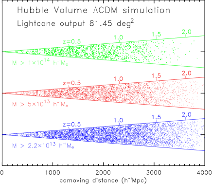
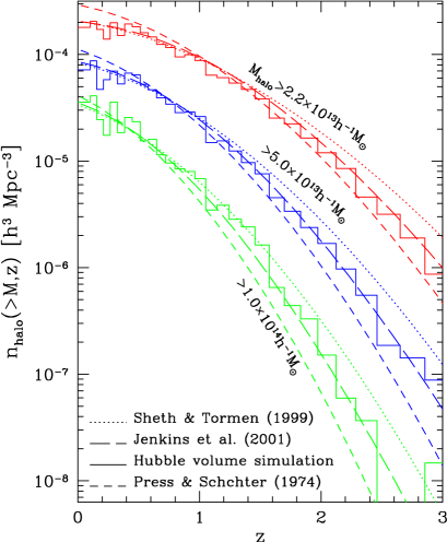
Figure 6.: Projected distribution of dark matter halos with $M_{\rm halo}>M_{\rm min}$ in the light-cone output of the Hubble volume simulation; $M_{\rm min}=1\times 10^{14}h^{-1}M_{\odot}$, $5\times 10^{13}h^{-1}M_{\odot}$ and $2.2\times 10^{13}h^{-1}M_{\odot}$ from top to bottom.

Figure 7.: Redshift distribution of the cumulative mass function of halos identified in the light-cone output of the Hubble volume simulation (histograms).

Figure 6 plots the projected distribution of identified halos from “light-cone output” of the Hubble Volume $\Lambda$CDM simulation (Evrard et al. 2002) with $\Omega_{\rm b}=0.04$, $\Omega_{\rm CDM}=0.26$, $\sigma_{8}=0.9$, $\Omega_{\Lambda}=0.7$ and $h=0.7$.

Figure 7 displays the redshift distribution of the cumulative mass functions of the identified halos with $M>2.2\times 10^{13}h^{-1}M_{\odot}$, $5.0\times 10^{13}h^{-1}M_{\odot}$, and $1.0\times 10^{14}h^{-1}M_{\odot}$. The total number of the corresponding halos at $0<z<3$ is 21,090, 5,554 and 1,543, respectively. For comparison, we also plot the predictions on the basis of the Press-Schechter mass function (short-dashed lines), the modified mass function by Sheth & Tormen (1999; dotted lines), and the fitting model by Jenkins et al. (2001; long-dashed lines). The Press-Schechter model underpredicts the halo abundance at $z>1$, while the Sheth-Tormen model overpredicts beyond $z\sim 1.5$. This tendency is consistent with the previous finding of Jenkins et al. (2001) that the Sheth-Tormen model overestimates the number of halos when ln($\sigma^{-1}$) becomes large.

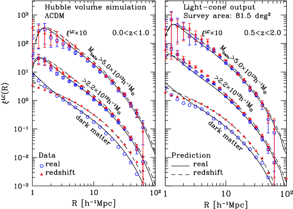
Figure 8.: Two-point correlation functions of halos on the light-cone; simulation results (symbols; open circles and filled triangles for real and redshift spaces, respectively) and our predictions (solid and dotted lines for real and redshift spaces, respectively). The error bars denote the standard deviation computed from 200 random re-samplings of the bootstrap method. The amplitudes of $\xi^{LC}$ for $M_{\rm halo}\geq 5.0\times 10^{13}h^{-1}M_{\odot}$ are increased by an order of magnitude for clarity.

Figure 8 compares our model predictions with the clustering of simulated halos. For the dark matter correlation functions, our model reproduces the simulation data almost perfectly at $R>3h^{-1}$Mpc (see also Hamana et al. 2001a). This scale corresponds to the mean particle separation of this particular simulation, and thus the current simulation systematically underestimates the real clustering below this scale especially at $z>0.5$. Our model and simulation data also show quite good agreement for dark halos at scales larger than $5h^{-1}$Mpc. Below that scale, they start to deviate slightly in a complicated fashion depending on the mass of halo and the redshift range. This discrepancy may be ascribed to both the numerical limitations of the current simulations and our rather simplified model for the halo biasing. Nevertheless the clustering of clusters on scales below $5h^{-1}$Mpc is difficult to determine observationally anyway, and our model predictions differ from the simulation data only by $\sim 20$ percent at most. Therefore we conclude that in practice our empirical model provides a successful description of halo clustering on the light-cone.

6. What’s next ? : dark halos vs. galaxy clusters

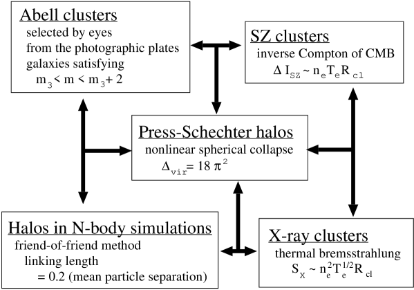
Figure 9.: Dark halos – galaxy clusters connection.

As I have briefly shown in the above sections, understanding of the density profiles and clustering of dark halos has been significantly advanced during last several years. With those theoretical/empirical successes in mind, the next natural question is how to apply them for the description of real galaxy clusters. In principle this may be fairly straightforward, but in reality the main obstacle is the lack of the proper definition of clusters. This point of view is clearly illustrated in Figure 9 which summarizes the conventional definitions of clusters/halos in various situations. There are a wide range of practical (and quite different!) definitions of dark halos and clusters of galaxies. Of course they are closely related, but the one-to-one correspondence is unlikely and nothing but a working hypothesis. We we need more quantitative justification or modification of the working hypothesis in order to move on to precision cosmology with clusters.

This problem has not been considered seriously probably because the agreement between model predictions and available observations seems already satisfactory. In fact, since current viable cosmological models are specified by a set of many adjustable parameters, the agreement does not necessarily justify the underlying assumption. Thus it is dangerous to stop doubting the unjustified assumption because of the (apparent) success.

Acknowledgments.

I would like to thank S. Bowyer and C.-Y. Hwang for inviting me to this well-organized and fruitful meeting. The plots that I presented in these proceedings are based on my collaborative work with A.E.Evrard, T.Hamana, Y.P.Jing, N.Makino, S.Sasaki and N.Yoshida. This research was supported in part by the Grant-in-Aid for Scientific Research of JSPS (12640231, 14102004).

References

Bartelmann, M., Huss, A., Colberg, J. M., Jenkins, A., & Pearce, F. R. 1998, A&A, 330, 1

Bullock, J. S., Kolatt, T. S., Sigad, Y., Somerville, R. S., Kravtsov, A. V., Klypin, A. A., Primack, J. R., & Dekel, A. 2001, MNRAS, 321, 559

Crone, M.M., Evrard, A.E., & Richstone, D. 1994, ApJ, 434, 402

Czoske, O., Moore,B., Kneib, J.-P. & Soucail, G. 2002, å, 386, 31

Davé, R., Spergel, D. N., Steinhardt, P.J., & Wandelt, B. D. 2001, ApJ, 547, 574

Davis, M. & Peebles, P. J. E. 1977, ApJS, 34, 425

de Blok, W. J. G., McGaugh, S. S., Bosma, A., & Rubin, V. C. 2001, ApJ, 552, L23

Evrard, A.E., MacFarland, T. J., Couchman, H. M. P., Colberg, J. M., Yoshida, N., White, S. D. M., Jenkins, A., Frenk, C. S., Pearce, F. R., Peacock, J. A., & Thomas, P. A. 2002, ApJ, 573, 7

Frenk, C.S., White, S.D.M., Davis, M., & Efstathiou, G. 1988, ApJ, 327, 507

Fukushige, T., & Makino, J. 1997, ApJ, 477, L9

Fukushige, T., & Makino, J. 2001, ApJ, 557, 533

Gunn, J.E. & Gott, J.R. 1972, ApJ, 176, 1

Gunn, J.E. 1977, ApJ, 218, 592

Hamana, T., Colombi, S., & Suto, Y. 2001a, A& A, 367, 18

Hamana, T., Yoshida, N., Suto, Y., & Evrard, A.E. 2001b, ApJ, 561, L143

Hernquist, L. 1990, ApJ, 356, 359

Hoffman, Y., & Shaham, J. 1985, ApJ, 297, 16

Jenkins, A., Frenk, C.S., White, S.D.M., Colberg, J.M., Cole, S., Evrard, A.E., Couchman, H.M.P. & Yoshida, N., 2001, MNRAS, 321, 372

Jing, Y. P., & Suto, Y. 2000, ApJ, 529, L69

Jing, Y. P., & Suto, Y. 2002, ApJ, 574, in press

Lee, J., & Suto, Y. 2002, in preparation

Li, L. X., & Ostriker, J. P. 2001, ApJ, 566, 652

Makino, N., Sasaki, S., & Suto, Y. 1998, ApJ, 497, 555

Matarrese, S., Coles, P., Lucchin, F., & Moscardini, L. 1997, MNRAS, 286, 115

Matsubara, T., Suto, Y., & Szapudi, I. 1997, ApJ, 491, L1

Meneghetti, M., Bolzonella, M., Bartelmann, M., Moscardini, L., & Tormen, G. 2000, MNRAS, 314, 338

Meneghetti, M., Yoshida, N., Bartelmann, M., Moscardini, L., Springel, V., Tormen, G., & White S. D. M. 2001, MNRAS, 325, 435

Miralda-Escudé, J. 2002, ApJ, 564, 60

Molikawa, K., & Hattori, M. 2001, ApJ, 559, 544

Moore, B., Governato, F., Quinn, T., Stadel, J., & Lake, G. 1998, ApJ, 499, L5

Moore, B., Quinn, T., Governato, F., Stadel, J., & Lake, G. 1999, MNRAS, 310, 1147

Moscardini, L., Coles, P., Lucchin, & F., Matarrese, S. 1998, MNRAS, 299, 95

Nakamura, T. T., Matsubara, T., & Suto, Y. 1998, ApJ, 494, 13

Navarro, J.F., Frenk, C.S., & White, S.D.M. 1995, MNRAS 275, 720

Navarro, J.F., Frenk, C.S., & White, S.D.M. 1996, ApJ, 462, 563

Navarro, J.F., Frenk, C.S., & White, S.D.M. 1997, ApJ, 490

Oguri, M., Taruya, A., & Suto, Y. 2001, ApJ, 559, 572

Peebles, P.J.E. 1970, AJ, 75, 13

Press, W. H., & Schechter, P. 1974, ApJ, 187, 425

Quinn, P.J., Salmon, J.K., & Zurek, W.H., 1986, Nature, 322, 32

Sheth, R.K., & Tormen, G. 1999, MNRAS, 308, 119

Spergel, D. N., & Steinhardt P. J. 2000, Phys.Rev.Lett, 84, 3760

Suginohara, T., Taruya, A., & Suto, Y. 2001, ApJ, 566, 1

Suto, Y. 1993, Prog. Theor. Phys., 90, 1173

Suto, Y., Magira, H., Jing, Y. P., Matsubara, T., & Yamamoto, K. 1999, Prog.Theor.Phys.Suppl., 133, 183

Suto, Y., Sasaki, S., & Makino, N. 1998, ApJ, 509, 544

Syer, D., & White, S.D.M. 1998, MNRAS, 293, 337

Takahashi, R., & Chiba, T. 2001, ApJ, 563, 489

Tyson, J. A., Kochanski, G. P., & Dell’Antonio I. P. 1998, ApJ, 498, L107

West, M.J., Dekel, A., & Oemler, A. Jr., 1987, ApJ, 316, 1

Yamamoto, K., & Suto, Y. 1999, ApJ, 517, 1

Yoshida, N., Springel, V., White, S.D.M., & Tormen, G. 2000, ApJ, 544, L87