Faint AGN and the Ionizing Background

Abstract

We determine the evolution of the faint, high-redshift, optical luminosity function of Active Galactic Nuclei (AGN) implied by several observationally-motivated models of the ionizing background from $3<z<5$. Our results depend crucially on whether we use the total ionizing rate measured by the proximity effect technique or the lower determination favored by the flux decrement distribution of Ly$\alpha$ forest lines. Assuming a faint-end luminosity function slope of 1.58 and the SDSS estimates of the bright-end slope and normalization, we find that the luminosity function must break at $M_{B}^{*}=-24.2,-22.3,-20.8$ at $z=3,4,5$ if we adopt the lower ionization rate and assume no stellar contribution to the background. The breaks must occur at $M_{B}^{*}=-20.6,-18.7,-18.7$ for the proximity effect estimate. Since stars may also contribute to the background, these values are lower limits on the break luminosity, and they brighten by as much as $\sim 2$ mag if the escape fraction of ionizing photons from high-z galaxies is consistent with recent estimates: $f_{\rm esc}=0.16$. By comparing our expectations to faint AGN searches in the HDF and high-z galaxy fields, we find that typically-quoted proximity effect estimates of the background imply an over-abundance of AGN compared to the faint counts (even with $f_{\rm esc}=1$). Even adopting the lower bound on proximity effect measurements, the stellar escape fraction must be high: $f_{\rm esc}\lower 0.43057pt\hbox{\hbox to0.0pt{\raise 2.58334pt\hbox{\hskip 1.29167pt{{$\scriptscriptstyle>$}}}\hss} \kern-1.72218pt{{$\scriptscriptstyle\sim$}}}0.2$. Conversely, the lower flux-decrement-derived background requires a smaller number of ionizing sources, and faint AGN counts are consistent with this estimate only if there is a limited stellar contribution, $f_{\rm esc}\lower 0.43057pt\hbox{\hbox to0.0pt{\raise 2.58334pt\hbox{\hskip 1.29167pt{{$\scriptscriptstyle<$}}}\hss} \kern-1.72218pt{{$\scriptscriptstyle\sim$}}}0.05$. Our derived luminosity functions together with the locally-estimated black hole density suggest that the efficiency of converting mass to light in optically-unobscured AGN is somewhat lower than expected, $\epsilon\lower 0.43057pt\hbox{\hbox to0.0pt{\raise 2.58334pt\hbox{\hskip 1.29167pt{{$\scriptscriptstyle<$}}}\hss} \kern-1.72218pt{{$\scriptscriptstyle\sim$}}}0.05$ (all models). Comparison with similar estimates based on X-ray counts suggests that more than half of all AGN are obscured in the UV/optical. We also derive lower limits on typical AGN lifetimes and obtain $\lower 0.43057pt\hbox{\hbox to0.0pt{\raise 2.58334pt\hbox{\hskip 1.29167pt{{$\scriptscriptstyle>$}}}\hss} \kern-1.72218pt{{$\scriptscriptstyle\sim$}}}10^{7}$yr for favored cases.

1 Introduction

Among the long-standing goals in extragalactic astronomy is to explain and characterize the population of Active Galactic Nuclei (AGN). Their large luminosities, compact sizes, and association with radio jets have lead to the assumption that AGN are powered by accretion onto supermassive black holes (Salpeter 1964; Zel’dovich & Novikov 1964; Lynden-Bell 1969). Although this framework provides a theoretical starting point, there are many questions that remain largely unresolved. These include explaining the origin of the central black holes (e.g. Eisenstein & Loeb 1995; Madau & Rees 2001; Koushiappas, Bullock, & Dekel 2002), understanding the fueling process, lifetime, and efficiency of the central engine (see, e.g. Rees 1984; Koratkar & Blaes 1999), and, ultimately, determining how quasar activity fits within our cosmological theory for structure formation.

For many years, the role of AGN in structure formation was believed to be that of a tracer population, important in their own right, but cosmologically interesting mainly for their contribution to the UV ionizing background (and in their ability to track the collapse of structure). Recent indications have changed this view dramatically. It now seems likely that AGN play an important role in the formation of galaxies. In a reversal of sorts, this paper focuses on using the observed ionizing emissivity at high-redshift in order to constrain the evolution of the AGN luminosity function. Derived in this way, our luminosity functions relate directly to the long-standing desire to pinpoint the dominant ionizing sources in the Universe, and additionally help constrain models that attempt to explain AGN within a cosmological context.

The AGN luminosity function has long served as a benchmark for understanding the formation and evolution of quasi-stellar objects (QSOs) (Efstathiou & Rees 1988; Carlberg 1990; Haehnelt & Rees 1993; Cavaliere, Perri & Vittorini 1997; Haiman & Loeb 1998; Richstone et al. 1998, Haehnelt, Natarajan, & Rees 1998; Cattaneo, Haehnelt, & Rees 1999; Haiman, Madau, & Loeb 1999, Kauffman & Haehnelt 2000; Haiman & Hui 2001; Haehnelt & Kauffman 2001; Steed, Weinberg, & Miralda-Escudé 2002). Recent indications that AGN activity is linked in a fundamental way with the formation of galaxies make these studies all the more relevant (Heckman et al. 1984; Sanders et al. 1988; Kormendy & Richstone 1995; Sanders & Mirabel 1996; Boyle & Terlevich 1998; Dickinson et al. 1998; Magorrian et al. 1998; Richstone et al. 1998; Laor 1998; Wandel 1999; van der Marel 1999; Franceschini et al. 1999; Mathur 2000; Canalizo & Stockton 2001; Levenson, Weaver, & Heckman 2001; Ferrarese 2002). Specifically, the relation between black hole mass and bulge velocity dispersion (Gebhardt et al. 2000a,  2000b; Ferrarese & Merritt 2000; Ferrarese et al. 2001) is so tight that it seems impossible to understand without some significant cross-talk (in the form of feedback) between the AGN phase and the formation of the galaxy and its stellar bulge.

Modelers attempting to understand these relations have been forced to test and refine their assumptions by comparing to the low-redshift AGN luminosity function, or to bright quasar counts at high-redshift, because the faint population of AGN is relatively unconstrained at high-$z$. This lack of knowledge about low-luminosity objects allows considerable, unwanted freedom for model builders. For example, Haiman & Loeb (1998) have explored the idea that faint AGN are linked in a simple way with low-mass cold dark matter (CDM) halos. This predicts a large number of low-luminosity systems at high-$z$ because less massive halos are relatively abundant at early times. Another possibility is that AGN activity in small halos is suppressed by feedback processes. A recent example of this idea is explored in Kauffman & Haehnelt (2000), who utilize a qualitatively plausible feedback scheme to model black hole properties and to match the observed evolution in AGN number density from $z\sim 0$ to $z\sim 2$. Because their model relies on feedback that scales with host population and redshift, a high-$z$ constraint on the number of dim objects would serve as a useful test.

The AGN luminosity function (LF) is typically written as $\phi(L,z)dL$, and is defined as the number of objects per unit comoving volume at redshift $z$, with luminosity between $L$ and $L+dL$. In the optical, the majority of studies use B magnitudes. So unless otherwise stated, $L$ will denote B band luminosity throughout this paper. For low-redshift AGN, $\phi$ is well represented by a broken power law

$$\phi(L,z)=\frac{\phi_{*}/L_{*}}{(L/L_{*})^{\gamma_{f}}+(L/L_{*})^{\gamma_{b}}},$$ (1)

which has a break at luminosity $L_{*}$, a characteristic number density $\phi_{*}$, and asymptotic faint and bright slopes of $\gamma_{f}$ and $\gamma_{b}$ respectively. As will be discussed in §2, out to $z\sim 2.5$ the AGN LF seems to evolve only in luminosity, in the sense that $L_{*}$ gets brighter with increasing $z$, while the other parameters stay fixed ($\gamma_{f}\simeq 1.6$, $\gamma_{b}\simeq 3.4$, and $\phi_{*}\simeq 10^{3}$Gpc^-3). This kind of evolution is known as pure luminosity evolution (PLE), and the current best-estimate for $L_{*}(z)$ under this assumption has it rising dramatically from its local value of $\sim 10^{11}L_{\odot}$ at $z=0$ to nearly $\sim 10^{13}L_{\odot}$ at $z=2.5$ (Boyle, Shanks, & Peterson 1988; Koo & Kron 1988; Hewett et al. 1993; Pei 1995a; Boyle et al. 2000). Beyond this redshift, only the brightest quasars have been observed in significant numbers, and there is as of yet no evidence for a break in the luminosity function. In terms of the double power-law (1), the high-$z$ observations only measure the bright-end slope $\gamma_{b}\simeq 2.6-2.9$ (Schmidt, Schneider & Gunn 1995, hereafter SSG; Fan et al. 2001a) and fix an overall integrated normalization that roughly imposes a constraint on the quantity $\phi_{*}L_{*}^{\gamma_{b}-1}$ as a function of z (see §2). Most interestingly, the space density of the observable bright quasars falls steadily from $z\sim 3$ out to $z\sim 6$ (Warren, Hewett, & Osmer 1994 [WHO94]; Kennefick, Djorgovski, & de Carvalho 1995 [KDC95]; SSG; Fan et al. 2001a), but this decline cannot be faithfully represented in terms of PLE, as the data shows $\gamma_{b}$ is flatter at early times. This leaves us at high redshift without a natural extension of the bright-end LF to fainter magnitudes. Presumably, future QSO surveys will detect a break in the LF at $z\lower 0.43057pt\hbox{\hbox to0.0pt{\raise 2.58334pt\hbox{\hskip 1.29167pt{{$\scriptscriptstyle>$}}}\hss} \kern-1.72218pt{{$\scriptscriptstyle\sim$}}}3$ and measure a faint-end slope. Until then, it is useful to examine other constraints.

A popular technique for constraining a population of unresolved sources is to set an upper limit based on their contribution to the diffuse background light. For instance, AGN are strong X-ray emitters, so measurements of the cosmic X-ray background might be used to provide upper bounds on the density of AGN. The problem with this is that the X-ray background is measured locally, and we are interested in constraining a high-$z$ population that contributes only a small fraction to the $z=0$ signal (see e.g. Hasinger 2002). What is preferable is a measurement of some background at high $z$ by an indirect method. It turns out that the UV ionizing background is ideal for this purpose. As discussed in §3, the hydrogen ionizing emissivity can be measured at high-redshift by studying Lyman alpha absorbers along the line of sight to distant quasars. This measurement is especially useful because the derived background at a specific redshift $z$ is roughly local: there is very little contribution from higher redshift sources because the mean free path to photo-electric absorption is short compared to cosmological distances (see Madau, Haardt, & Rees 1999 [MHR] and our Appendix).

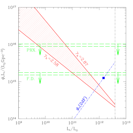
Figure 1: Schematic representation of the limits on $\phi_{*}$ and $L_{*}$ for $z=4$. The integrated LF ($\Phi(<M_{B})$) basically constrains $\phi_{*}L_{*}^{\gamma_{b}-1}$. We assume that all reasonable choices (shaded region) for the bright-end slope are bracketed by the values from SSG (2.87) and SDSS (2.58). Since the observations at high redshift show no sign of a break for $M_{B}\lesssim-26$, we do not consider this area of parameter space (vertical line). The filled square is the point in parameter space consistent with both the integrated LF and the parameters from 2dF (i.e. $\gamma_{b}=3.41$ and $\phi_{*}=1070\rm{Gpc}^{-3}$). We also bring in upper limits from ionizing background measurements: proximity effect (“PRX.”) and flux decrement (“F.D.”).

In what follows we use this idea to construct AGN luminosity functions that reproduce the ionizing background measurements, allowing in some cases for significant contributions from other sources (e.g. stars). We can demonstrate our general program using some simple approximations. Let us assume (as we do throughout) that we can approximate each AGN as emitting light with a self-similar spectrum that varies only in normalization from object to object (§2.2). This implies a fixed ratio between an AGN’s specific luminosity at the $912\mbox{\AA}$ Lyman edge to its luminosity in the B-band: $\eta_{\nu}\equiv L_{\nu}/L\simeq 10^{18}$ erg/s/Hz/L_⊙. The comoving emissivity at the Lyman edge is then: $\varepsilon_{\nu}=\eta_{\nu}\ell$, where $\ell$ is the luminosity density of AGN (in the B-band). For a reasonable LF, $\ell$ will be dominated by objects near the break, so we expect $\ell\sim\phi_{*}L_{*}$, or $\varepsilon_{\nu}\sim\eta_{\nu}\phi_{*}L_{*}$ . A slightly more accurate estimate of $\ell$ comes from integrating the LF (1) from $L=0$ to $\infty$, and with this we obtain $\varepsilon_{\nu}\simeq\eta_{\nu}\phi_{*}L_{*}[(2-\gamma_{f})^{-1}+(\gamma_{b}-2)^{-1}]$. Thus, a measurement of the ionizing emissivity at some redshift mostly constrains the parameter combination $\phi_{*}L_{*}$, with a weak dependence on the LF slopes (as long as neither slope approaches $2$). Direct observations, on the other hand, measure the bright-end slope $\gamma_{b}$ and fix the normalization of the bright-end tail. Together, then, the limits from $\varepsilon_{\nu}$ and direct observations can effectively restrict the acceptable values of $\phi_{*}$ and $L_{*}$.

A schematic illustration of this is shown in Figure 1, where we plot the available parameter space at $z=4$. Direct observations of the density of bright QSOs leads to a constraint of $\phi_{*}L_{*}\propto L_{*}^{2-\gamma_{b}}$ (see §2.1), which we draw (diagonal lines) for two values of $\gamma_{b}$ from separate surveys (2.87 from SSG; 2.58 from Fan et al. 2001a). We presume that the best estimate of the bright-end slope lies between these two measurements, and therefore, that the values of $\phi_{*}$ and $L_{*}$ are situated somewhere in the shaded region. The fact that the break has not yet been observed down to the limiting magnitude $L_{\rm lim}\simeq 10^{12.6}L_{\odot}$ of SDSS allows us to set an upper limit on $L_{*}$ (vertical line). We can further narrow down the parameter space with two different (conflicting) measurements of the ionizing emissivity at the same redshift (the higher line comes from the proximity effect and the lower line comes from the flux decrement distribution, as discussed in §3). We draw these as upper limits (horizontal bands), since contributions to the background from non-AGN sources will require fewer AGN, further restricting the allowed range of $\phi_{*}L_{*}$. The width of the bands reflects the slight dependence of the emissivity on $\gamma_{b}$. As for the faint-end slope, we have fixed it to the low redshift value of 1.58, but we explore other values of $\gamma_{f}$ in §5.1. What is evident in the figure is the fact that the emissivity measurements provide an extremely useful limit on the parameter space left available from the direct observations of bright QSOs.

In the next section we review what is known about the optical luminosity function from direct observations, and discuss some possible caveats associated with dust and gravitational lensing. We also discuss our assumed template AGN spectrum. In §3 we review the different ionizing background measurements, and in §4, we describe our calculation of the AGN contribution to the background as well as the contribution from stars and IGM reemission. We present our results in §5 for three separate models of AGN emissivity, and we compare the derived LFs to past and future faint surveys. In §6 we discuss our results in the context of other constraints on the relative AGN and stellar emissivities at high-$z$. We also examine what our results imply for the AGN efficiencies and lifetimes. Our conclusions are summarized in §7

Unless otherwise stated, we assume that the cosmology is one with the universe made flat by a cosmological constant $\Omega_{m}=1-\Omega_{\Lambda}=0.4$, and that the Hubble parameter at $z=0$ is $H_{0}=65$ km s^-1 Mpc^-1.

2 AGN Properties: Composite Spectra and Observed Luminosity Function

In this section we will discuss the empirical AGN luminosity function (LF) and go on to present our assumed template spectral energy distribution, which allows us to calculate the ionizing emissivity for any given $\phi(L,z)$. As mentioned previously, $L$ will always have units B-band solar luminosities. We assume that the spectrum of an AGN varies only in normalization from object to object, and we present our assumed distribution in terms of specific luminosity $L_{\nu}$ in units of erg/s/Hz.

2.1 Empirical AGN Luminosity Function

In §1 we discussed how low-redshift observations indicate that the AGN luminosity function is well-described by a double power law shape given by Eq. 1. Although yet to be confirmed by observations, we will assume that this shape provides a useful characterization of the LF at all redshifts. Under this premise, the AGN LF has four main parameters that must be described at each $z$: $\gamma_{f}$, $\gamma_{b}$, $\phi_{*}$, and $L_{*}$.

Detecting AGN at low redshift is done primarily by selecting for strong UV emitters (e.g. Hartwick & Schade 1990; Hewett et al. 1995). The largest survey to date is that of the 2dF (Boyle et al. 2000), which tracks the evolution of QSOs over the redshift range $0.35<z<2.3$. Their data is consistent with the assumption of pure luminosity evolution (PLE). Under PLE, all of the LF evolution is contained in $L_{*}$, while the shape ($\gamma_{f}$, $\gamma_{b}$) and normalization ($\phi_{*}$) remain constant. Their fit for a $\Lambda$CDM cosmology has $\gamma_{f}=1.58$, $\gamma_{b}=3.41$, $\phi_{*}=1070\rm{Gpc}^{-3}$, and $\log_{10}(L_{*})=11.24+1.36z-0.27z^{2}$. The rapid rise in $L_{*}(z)$ characterizes an increase in the number density of AGN as we look to higher $z$. We plot the 2dF fit in Figure 2 for several redshifts. For reference, we have only plotted the fits over the range of (absolute) luminosities probed by the 2dF. The rapid evolution and characteristic LF shape found by the 2dF for $z\lower 0.43057pt\hbox{\hbox to0.0pt{\raise 2.58334pt\hbox{\hskip 1.29167pt{{$\scriptscriptstyle<$}}}\hss} \kern-1.72218pt{{$\scriptscriptstyle\sim$}}}2.5$ is consistent with previous work in overlapping redshift ranges (see e.g. Pei 1995a).

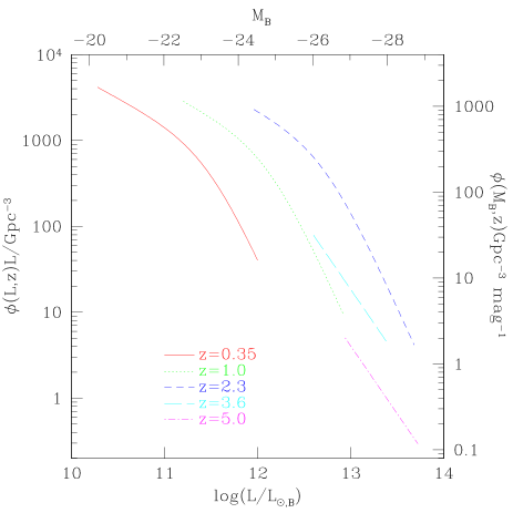
Figure 2: Fits to the observed LF for several redshifts. The three lowest redshift measurements come from Boyle et al. (2000) for $16.50\lesssim M_{B}\lesssim 20.85$. The two highest come from Fan et al. (2001a) for $18\lesssim i^{*}\lesssim 20$.

Beyond $z\sim 2.5$, however, our knowledge about the AGN population is much less complete. The information we do have is based on the bright end of the LF, which is observed to fall off gradually out to $z\lower 0.43057pt\hbox{\hbox to0.0pt{\raise 2.58334pt\hbox{\hskip 1.29167pt{{$\scriptscriptstyle>$}}}\hss} \kern-1.72218pt{{$\scriptscriptstyle\sim$}}}5$ (WHO94, SSG, Fan et al. 2001a,b). Of course, if PLE holds to high-$z$ then the evolution of the brightest quasars is sufficient to define the entire LF evolution. For example, under the PLE assumption, Pei (1995a) and later MHR used the observed bright-end evolution (along with low-$z$ data compilations) to extrapolate the evolution of the AGN LF out to high-$z$. Models of this kind have been popular for estimating the number of high-redshift AGN and calculating expected AGN contribution to the ionizing background. Yet even before the most recent SDSS data, there were indications that the PLE assumption might break down at early times. Specifically, the bright-end slope obtained by SSG (and by KDC95 at slightly larger magnitudes) is flatter ($\gamma_{b}\simeq 2.9$) than that measured for local AGN. The recent SDSS data (Fan et al. 2001a) reveal an even flatter bright-end slope ($\gamma_{b}\simeq 2.6$) for $3.5\lower 0.43057pt\hbox{\hbox to0.0pt{\raise 2.58334pt\hbox{\hskip 1.29167pt{{$\scriptscriptstyle<$}}}\hss} \kern-1.72218pt{{$\scriptscriptstyle\sim$}}}z\lower 0.43057pt\hbox{\hbox to0.0pt{\raise 2.58334pt\hbox{\hskip 1.29167pt{{$\scriptscriptstyle<$}}}\hss} \kern-1.72218pt{{$\scriptscriptstyle\sim$}}}5.0$. And although not as statistically significant, the data at slightly fainter magnitudes from the Isaac Newton Telescope Wide Angle Survey (Sharp et al. 2001) are consistent with the results from SDSS only if $\gamma_{b}\lower 0.43057pt\hbox{\hbox to0.0pt{\raise 2.58334pt\hbox{\hskip 1.29167pt{{$\scriptscriptstyle<$}}}\hss} \kern-1.72218pt{{$\scriptscriptstyle\sim$}}}2.9$. All together, these observations provide strong evidence that the LF evolves in shape as well as in luminosity, and therefore PLE does not extend to high redshift. In this case, constraints on the faint-end of the LF become all the more valuable.

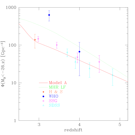
Figure 3: The number density of bright quasars for $z\gtrsim 3$. The solid line is one of our models constrained to fit the SDSS data, and the dot-dash line is the PLE LF from MHR. The data points are from Hartwick & Schade (1990), Warren, Hewett, Osmer (1994), Schmidt, Schneider, Gunn (1995) and SDSS (Fan et al. 2001a). Since all the of the compiled data sets assume $\Omega_{M}=1$, we have scaled our fit to match this cosmology. Note also that for Hartwick & Schade and Warren, Hewett, Osmer the error bars are summed over the differential LF uncertainties and, therefore, are likely overestimated.

We will normalize all of our high-$z$ LF models to match the SDSS results (Fan et al. 2001a,b) over the range in $L$ that they are measured. The best-fit LF of Fan et al. is shown in Figure 2 for $z=3.6$ and $5.0$ over the relevant range of absolute magnitudes. The best-fit bright-end slope is $\gamma_{b}=2.58$ (the quoted error is $\pm 0.23$) and the number density evolution over the redshift range $3.5\lower 0.43057pt\hbox{\hbox to0.0pt{\raise 2.58334pt\hbox{\hskip 1.29167pt{{$\scriptscriptstyle<$}}}\hss} \kern-1.72218pt{{$\scriptscriptstyle\sim$}}}z\lower 0.43057pt\hbox{\hbox to0.0pt{\raise 2.58334pt\hbox{\hskip 1.29167pt{{$\scriptscriptstyle<$}}}\hss} \kern-1.72218pt{{$\scriptscriptstyle\sim$}}}6.0$ follows the integrated constraint

$$\Phi(M_{B}<-26,z)=10^{1.99-0.47(z-3)}\ \rm{Gpc}^{-3},$$ (2)

where

$$\Phi(<M_{B},z)=\int^{\infty}_{L(M_{B})}\phi(L,z)dL,$$ (3)

and $\log L(M_{B})=-0.4(M_{B}-M_{\odot,B})$. Note that for $\gamma_{b}>1$ and $L(M_{B})\gg L_{*}$ the integral (3) approximates to $\simeq\phi_{*}(L_{*}/L_{m})^{\gamma_{b}-1}/(\gamma_{b}-1)$. The parameterized normalization from the SDSS work is shown in Fig. 3 along with data from several other high redshift surveys. Except for the seemingly anomalous point from WHO94 at $z=3.2$, all the integrated LF measurements appear to agree. The figure also illustrates how the PLE model of MHR disagrees with the recent data, and highlights the need to reconsider the AGN contribution to the ionizing background at high-$z$. In what follows we will use the SDSS result to fix the bright-end slope and normalization of our constrained AGN LFs.

Before going on, we should address possible selection effects which could affect the empirical LF at high redshift. One possibility is that dust, both intrinsic to the host galaxy and in the foreground, may be affecting the observed evolution as well as shape of the AGN LF. For example, Fall & Pei (1993) showed that damped Ly$\alpha$ systems (DLAs) could be blocking 10-70% of the bright optical QSOs at $z\sim 3$. But the CORALS survey (Ellison et al. 2001) found that the distribution of DLAs was basically the same in both radio and optically selected QSO samples. Since dust should not affect radio wavelengths, this implies that intervening dust is not a significant bias. Moreover, Fan et al. (2001a) find the distribution of spectral indices in the SDSS sample is similar to that at low redshift, which would be unlikely if there was a substantial amount of dust along the line of sight. So too, any increase in reddening with redshift would presumably be at odds with the close agreement in LF evolution from surveys with very different selection techniques: the broad-band color selection in SDSS; the Ly$\alpha$-emission selection of SSG; and even radio selection (e.g. Hook, Shaver & McMahon 1998), which should be representative of full sample, assuming that the ratio of radio-loud to radio-quiet QSOs is redshift independent (Stern et al. 2000). However, none of this would seem to preclude the existence of a distinct population of highly extinguished QSOs, only observable in the X-ray (and perhaps the IR). We come back to this possibility when we address the relic black hole density in §6.2.

Another effect that could distort the LF is gravitational lensing (see Blandford & Narayan 1992 and references therein). Because of the shape of the LF, the magnification bias is stronger for more luminous objects, i.e. it is more likely that the bright-end of the LF is contaminated by artificially brightened AGN. According to Pei (1995b), the number of objects observed with $L=10L_{*}$ that are lensed could be as much as 44% at $z=3$ and 68% at $z=5$. However, these large lens fractions come from models that assume a now unreasonable density of compact objects (on the order of 10% the critical density). More recent estimates of the fraction of lensed objects in magnitude limited surveys are less than $\sim 20\%$ (Barkana & Loeb 2000; Wyithe & Loeb 2002). Because these are relatively small corrections, we will ignore the effect of magnification bias in our bright-end normalizations. However, it should be pointed out that the lens fraction gets larger the farther an observed luminosity is above the break. That is, the probability that the QSOs observed in the SDSS ($L\gtrsim 10^{12.5}\rm{L_{\odot,B}}$) are lensed increases the smaller $L_{*}$ turns out to be. In our emissivity constrained models (see Figure 1), we explore break luminosities that are several orders of magnitude below those investigated by Pei (1995b). However, these values of $L_{*}$ are probably unrealistic because they seem to be in conflict with some of the faint AGN searches (see §5).

2.2 Lyman Limit emissivity and Composite Spectra

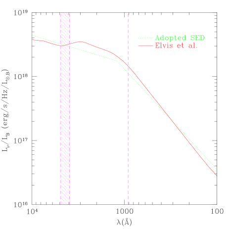
Figure 4: Our assumed template AGN spectrum shown along with the composite spectrum of Elvis et al. (1994). For reference, we have drawn vertical lines at the Lyman limit and a shaded band to indicate the wavelength range of the B-band.

Given an optical AGN LF $\phi(L,z)$, we are concerned with calculating the implied emissivity of ionizing photons. If $\varepsilon(\nu,z)$ is the comoving emissivity of photons at frequency $\nu$ and redshift $z$, then we can write

$$\varepsilon(\nu,z)=\int^{\infty}_{L_{\rm min}}dL\cdot\phi(L,z)\cdot L_{\nu}(L,\nu).$$ (4)

Here (and throughout this work) we adopt a minimum AGN luminosity $L_{\rm min}=10^{8}\rm{L_{\odot,B}}$ (or $M_{B}=-14.5$). This choice is comparable to the nuclear luminosity of the faintest Seyferts (Londish et al. 2000). Fortunately, the choice of $L_{\rm min}$ does not strongly affect our results as long as $L_{\rm min}\ll L_{*}$. Expression 4 provides a link between the emissivity and $\phi(L,z)$, once we specify the input spectrum, $L_{\nu}(L,\nu)$. We will assume that, on average, the specific luminosity of an AGN (as a function of frequency $\nu$) varies only in normalization such that $L_{\nu}\propto L$, with no $z-$dependence (see Kuhn et al. 2001).

From the UV to optical, an AGN spectrum, $L_{\nu}$, is reasonably well approximated by a double power law with a break near Ly$\alpha$ at $1216\mbox{\AA}$. Since the Galaxy is opaque to UV photons, we must rely on high redshift quasars to determine a typical quasar spectrum short-ward of the Lyman limit. For $\lambda<1200\mbox{\AA}$, we will use results from the most recent UV survey from HST (Telfer et al. 2002). Telfer and collaborators find that the specific luminosity of (radio quiet) AGN scales as $L_{\nu}\propto\nu^{-\alpha_{UV}}$, $\alpha_{UV}=1.57\pm 0.17$, from $\lambda\sim 500$ to $\sim 1200\mbox{\AA}$. Long-ward of Ly$\alpha$, we use the result of Vanden Berk et al. (2001), who relied on a composite of quasar spectra from the SDSS to determine $L_{\nu}\propto\nu^{-0.44}$ from $1200\mbox{\AA}$ to $\sim 5000\mbox{\AA}$.

Figure 4 shows our assumed spectrum compared to the composite spectrum of Elvis et al. (1994). The specific luminosity is normalized relative to the B-band luminosity $L$. For our B-band transformation we follow SSG and use $M_{B}=M_{AB}(4400\mbox{\AA})+0.12$. Of course, what we are mainly interested in is the ratio of $L_{\nu}$ at $912\mbox{\AA}$ ($\nu=\nu_{H}$) to the optical luminosity $L$, which for our spectrum is

$$\eta_{\nu}\equiv\frac{L_{\nu}(\nu_{\rm{H}})}{L}=10^{18.05}\ \rm{\frac{ergs/s/Hz}{L_{\odot,B}}}.$$ (5)

From combining the optical and UV power laws, we estimate an uncertainty in $\eta_{\nu}$ of $\pm 0.10$ in the exponent. This level of variation will not strongly affect our conclusions. For reference, the value implied by Elvis et al. (1994) is $\eta_{\nu}=10^{18.15}$ in the same units, and the value obtained by Shull et al. (1999) using a sample of 27 Seyferts is $\eta_{\nu}=10^{17.93\pm 0.04}$. Note that Shull et al. also find a slight luminosity dependence on this ratio, but we will ignore that possibility here. With our assumed $L_{\nu}$ spectrum, Expression 4 fully describes the relationship between a given optical LF and the ionizing emissivity as a function of redshift.

3 Ionizing Background Measurements

From the Gunn-Peterson effect (Gunn & Peterson 1965), it is clear that the IGM is highly ionized. If it can be assumed that this high ionization state is due to photo-ionization (as opposed to collisional excitation), then measurements of the IGM, particularly the Ly$\alpha$ forest, can reveal information on the nature of the ionizing background. We can characterize this background with the hydrogen ionization rate:

$$\Gamma(z)=4\pi\int^{\infty}_{\nu_{\rm{H}}}d\nu\frac{J(\nu,z)}{\nu}\sigma_{\rm{H}}(\nu).$$ (6)

Here the cross section to hydrogen photo-electric absorption is $\sigma_{\rm{H}}=6.35\times 10^{-18}\rm{cm}^{2}\cdot(\nu/\nu_{\rm{H}})^{-3}$ and $J(\nu,z)$ is the background intensity (in units of $\rm{ergs/s/cm^{2}/Hz/sr}$). As will be discussed in the next section, the ionizing intensity relates simply to the AGN (and stellar) emissivity, $J(z)\propto\varepsilon(z)$, so we may approximate the spectrum of background intensity as $J\propto\nu^{-\alpha_{UV}}$. With this approximation we obtain:

$$\Gamma_{-12}(z)=\frac{12.0}{3+\alpha_{UV}}\ J_{-21}(z)$$ (7)

where $J_{-21}(z)\equiv J(\nu_{\rm{H}},z)$ in units of $10^{-21}\rm{ergs/s/cm^{2}/Hz/sr}$ and $\Gamma_{-12}\equiv\Gamma/10^{-12}\rm{s^{-1}}$. If there were only a single dominant source to the background (e.g. QSOs), then we could take $\alpha_{UV}$ to be equal to the typical spectral index of that source population. We will however be exploring cases where there are more than one dominant type of emitters, and so we will not immediately assume a value of $\alpha_{UV}$. For this reason, in the next section, we will quote measurements of the ionizing background using $\Gamma_{-12}$ (instead of $J_{-21}$).

Under the assumption of photo-ionization equilibrium, $\Gamma$ should scale as the ratio of ionized to neutral hydrogen ($n_{\rm{HII}}/n_{\rm{HI}}$). Given this ratio one may infer a value for $\Gamma$. At high-$z$, two techniques exist for measuring the amount of neutral hydrogen, and they both rely on using Ly$\alpha$ lines in the spectra of distant QSOs. One technique relies on analytic modeling of the expected distribution of lines in the vicinity of a QSO (the proximity effect) and the other uses hydro-dynamical simulations to model the expected distribution of lines along the line of sight to the quasar (what we will call the “flux decrement” analysis). We use the following two subsections to summarize the results of each technique.

3.1 Proximity effect

The proximity effect was first discussed by Bajtlik, Duncan, & Ostriker (1988). The technique relies on the observed decrease in the number of Ly$\alpha$ lines in the vicinity of a QSO relative to what one would have expected in the absence of the QSO. In principle, this decrease is a result of ionizing radiation from the QSO itself, which tends to reduce the neutral fraction in nearby absorbers. The number of observable lines should decrease correspondingly. An estimate of the ionizing rate can be obtained by determining the distance from the quasar at which the number of lines is equal to the background expectation. Over the years, measurements of $J_{-21}$ (assuming $\alpha_{UV}\sim 1.8$) have taken values between $\sim 0.7$ and $\sim 3$ (Williger et al. 1994; Bechtold 1994; Fernández-Soto et al. 1995; Cristiani et al. 1995; Giallongo et al. 1996; Cooke, Espey & Carswell 1997; Scott et al. 2000; Liske & Williger 2001). Since what is effectively measured is a ratio of proper distances, this analysis should be relatively independent of cosmological parameters. Most estimates of the proximity effect assume that the background is constant over the redshifts being sampled, so this technique does not appear to uniquely determine the evolution of $\Gamma_{-12}(z)$. Haardt & Madau (1996) and Fardal et al. (1998) have tried to fit the whole set of proximity effect measurements with a Gaussian. Scott et al. (2000) claim that their observations are well fit by the following parameterization from Fardal et al. (1998):

$$\Gamma_{-12}(z)=1.2(1+z)^{0.58}\exp\left[\frac{-(z-2.77)^{2}}{2.38}\right].$$ (8)

This fit is represented by the dot-dashed line in Figure 5.

There is some concern that the value of $\Gamma_{-12}$ determined from the proximity effect is overestimated. This is because QSOs are likely to be found in environments that are denser than average (Pascarelle et al. 2001; Ellison et al. 2002), so that the regions of excess ionization end up being smaller than they would have been if the region was of average density. Such overdensities would likely scale with the mass/luminosity of the AGN, which might explain the slight anti-correlation between more luminous QSOs and their proximity effects (see Cooke, Espey & Carswell 1997). Loeb & Eisenstein (1995) claim this bias could cause the proximity effect measurements to overestimate the background by as much as a factor of 3. The flux decrement technique discussed in the next subsection does in fact yield a lower ionizing background than the proximity effect, as would be expected if these concerns are valid. However, we will keep an open mind about the issue and discuss the constraints on faint AGN associated with each technique separately.

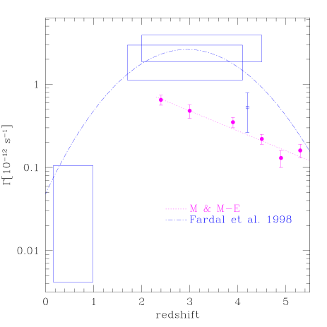
Figure 5: The ionizing rate as a function of redshift. The solid dots are from hydro-simulations by McDonald & Miralda-Escudé(2001). A linear fit has been drawn through the points. The solid boxes and open square are representative of recent proximity effect measurements (see Scott et al. 2000), where we have used the conversion $\Gamma_{-12}=2.64\cdot J_{-21}$ from Fardal et al. (1998). We have also drawn the Gaussian fit to this data from Fardal et al.

3.2 Flux Decrement

Another way to utilize the Ly$\alpha$ forest to measure the ionizing background requires making a theoretical prediction as to the amount of (unobserved) ionized hydrogen in each “cloud” along the line of sight to a quasar. This can be done using CDM theory (and N-body codes) coupled with hydrodynamical simulations that model gas evolution (Cen et al. 1994; Zhang et al. 1995; Hernquist et al. 1996; Miralda-Escudé et al. 1996; Rauch et al. 1997; Davé et al. 1997; Wadsley & Bond 1996; Zhang et al. 1998; McDonald et al. 2000). These simulations essentially generate a distribution of hydrogen Ly$\alpha$ optical depths which can be mapped to a distribution of flux decrements ($F=\exp(-\tau)$). The distributions generated in this way convincingly reproduce observations, adding to the long list of successes for the CDM paradigm. Although the shape of the flux decrement distribution depends upon details of the cosmology as well as models for the temperature-density relation, the normalization is proportional only to the baryon density, the ionization rate, and the Hubble parameter:

$$\tau\propto\frac{(\Omega_{b}h^{2})^{2}}{\Gamma(z)\ H(z)}.$$ (9)

Often times this relation is used to put constraints on $\Omega_{b}h^{2}$ (e.g. Hui et al. 2002). But McDonald & Miralda-Escudé (2000) [hereafter M&M-E] assume the baryon fraction from BBN: $\Omega_{b}h^{2}=0.02$ (Walker et al. 1991; Burles & Tytler 1998), so as to measure $\Gamma(z)$ from a sample of QSO spectra. In a $\Lambda$CDM cosmology, over the redshift range of $\sim 2.3-5$, their results can be approximated by

$$\Gamma_{-12}(z)=10^{-0.24z+0.4}.$$ (10)

We plot this flux-decrement result along with the proximity effect results in Figure 5. The flux decrement determination is a factor of $\lower 0.43057pt\hbox{\hbox to0.0pt{\raise 2.58334pt\hbox{\hskip 1.29167pt{{$\scriptscriptstyle>$}}}\hss} \kern-1.72218pt{{$\scriptscriptstyle\sim$}}}4$ below that of the proximity effect. We discuss how these differences affect constraints on the AGN LF in §5.

4 The IGM: AGN and stars as ionizing sources

Now that we have measurements of the background ionization rate, we need to relate them to the LF. This relation comes about via Eq. 7 which connects $\Gamma$ to the ionizing intensity. In principle, the intensity at any time is made up of the integrated contribution of all sources over the history of the universe. However, as discussed in detail by MHR, the contribution from distant sources is significantly degraded by attenuation. The intensity can be written as an integral over the (comoving) emissivity of sources as a function of redshift:

$$J(\nu,z)=\frac{c}{4\pi}\cdot(1+z)^{3}\cdot\int^{\infty}_{z}d\bar{z}\frac{dt}{d\bar{z}}\cdot\varepsilon(\bar{\nu},\bar{z})\cdot\rm{e}^{-\tau_{\rm eff}(\nu,z,\bar{z})},$$ (11)

where $\bar{\nu}=\nu\ (1+\bar{z})/(1+z)$, and $\tau_{\rm eff}$ is the effective optical depth due to photo-electric absorption in the IGM. In the Appendix we discuss how we model the IGM and $\tau_{eff}$ following the prescription of MHR. In practice we calculate $J$ using the full integral expression, but for purposes of illustration, it is useful to make the following approximation. If we assume that only ionizing sources within one absorption length, $\Delta l$ (where $\tau_{\rm eff}(\Delta l)\equiv 1$), contribute to the background, then Eq. 11 reduces to $J(\nu,z)\simeq(1+z)^{3}\varepsilon_{\nu}(z)\Delta l/4\pi$. At the Lyman edge, our adopted IGM model (Appendix) gives $\Delta l\simeq 39\rm{Mpc}[(1+z)/4]^{-4.5}$. Since $\Delta l\ll c/H(z)$ this is often called the “local source” approximation, and it yields:

$$J_{-21}(z)\simeq 0.17\ (1+z)^{-1.5}\ \varepsilon_{24}(\nu_{H},z).$$ (12)

Here we have introduced the symbol $\varepsilon_{24}$ which is the emissivity in units of 10²⁴ ergs/s/Hz/Mpc³.

Equations 11 and 7 allow us to relate an observed ionization rate $\Gamma(z)$ to a background ionizing emissivity $\varepsilon(z)$. However, the relation depends sensitively on the spectral slope of the background: $\Gamma\propto J/(3+\alpha_{UV})\propto\varepsilon/(3+\alpha_{UV})$. Because the far-UV slopes of galaxies and AGN are significantly different, deriving a limit on the background emissivity based on the ionization rate would necessitate assuming something about the background population. We would prefer a more general parameter that allows us to consider stars as well as AGN as major contributors to the background. For this purpose we propose the following “weighted” emissivity parameter

$$\hat{\varepsilon}^{i}\equiv\frac{\varepsilon_{24}^{i}(\nu_{H})}{3+\alpha_{UV}^{i}},$$ (13)

which facilitates a fair comparison between different populations, $i$. This definition allows us to rewrite the (approximate) Equation 12 as

$$\Gamma_{-12}(z)\simeq 2.0\ (1+z)^{-1.5}\ \sum_{i}\hat{\varepsilon}^{i}(z),$$ (14)

where the sum is over all populations of ionizing ionizing sources, $i=$ AGN, stars, reemission, etc. This expression can be rearranged to place an upper limit on the weighted emissivity coming from any individual population. In particular, we are concerned with limiting the emissivity from AGN:

$$\hat{\varepsilon}^{Q}(z)\ \simeq\ 0.5\ \Gamma_{-12}(z)\ (1+z)^{1.5}\ -\ [\hat{\varepsilon}^{*}(z)+\hat{\varepsilon}^{R}...].$$ (15)

The bracketed terms on the right hand side are included to illustrate how the allowed AGN emissivity is reduced by the presence of additional contributing populations. For example, $\hat{\varepsilon}^{*}$ represents the weighted emissivity from stars (see §4.1) and $\hat{\varepsilon}^{R}$ represents the contribution from cloud reemission (see §4.2). The contribution from clusters of galaxies is likely negligible (Randall & Sarazin 2000).

Fig. 6 illustrates the upper limit on weighted AGN emissivity $\hat{\varepsilon}$ imposed by the proximity effect (short dashed line) and flux decrement (long-dashed line) measurements of $\Gamma(z)$. As will be the case throughout, we have used the full integral expression given by Eq. 11 in order to place limits on the weighted emissivity (as opposed to the approximate expressions used for illustrative purposes in Eqs. 12, 14, and 15). However, in the language of Eq. 15, these two constraints amount to setting all of the bracketed (non-AGN) emissivities to zero. The thin solid line (Model A), on the other hand illustrates how the flux-decrement-derived limit on the AGN emissivity changes if we include a (conservative) estimate of the stellar emissivity, $\hat{\varepsilon}^{*}$. We describe this estimate in the next subsection. For reference we show the contribution to $\hat{\varepsilon}$ arising from AGN that have been directly observed by the 2dF at low-$z$ (bold solid line), and by SSG and the SDSS at high-$z$ (data points).

We now go on to discuss our stellar emissivity estimate in more detail.

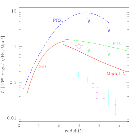
Figure 6: The weighted emissivity: $\varepsilon(\nu_{\rm{H}})/(3+\alpha_{UV})$. The bold solid line is the weighted emissivity implied by observed QSOs ($-26<M_{B}<-23$) from 2dF (Boyle et al. 2000). The crosses are from SSG and the triangles are from the SDSS (Fan et al. 2001a), both involving a conversion from $\Phi(M_{B}<-26)$. The star is the weighted LBG emissivity from Steidel et al. (2001). Limits have been drawn from the two ionization rate measurements: proximity effect (PRX.) and flux decrement (F.D.), see §3.1 and §3.2. We have also included our Model A (solid line), which is the allowed AGN emissivity accounting for a stellar contribution to the flux-decrement-derived background (see §5).

4.1 Emission from Galaxies

In addition to AGN, star-forming galaxies are an obvious contributor to the ionizing continuum. At energies above the Lyman edge, a star-forming galaxy spectrum is dominated by hot, short-lived O stars ($t_{\rm O}\lesssim 10^{7}\rm{yr}$). Theoretically, the number of Lyman continuum photons emitted by an (unobscured) $L_{*}$ galaxy should be about $10^{-3}$ smaller than the number emitted from an $L_{*}$ AGN (Madau & Shull 1996). However, the space density of $L_{*}$ galaxies is a factor of $\sim 10^{4}$ higher than that of $L_{*}$ AGN at $z\sim 0$, so stars could conceivably dominate the ionizing background. What mitigates this calculation is the fraction of Lyman continuum photons that can actually escape from the galaxy, $f_{\rm esc}$.

Theoretically, cold gas in a galaxy could trap most of the Lyman continuum emission (e.g. Haehnelt et al. 2001 and references therein). In agreement with this expectation, most local searches for Lyman continuum emission from galaxies have come up empty. At low redshift, using the Hopkins Ultraviolet Telescope, Leitherer et al. (1995) found that nearby starburst galaxies had a very small escape fraction, $f_{\rm esc}<3\%$ (see also Hurwitz et al. 1997). Similar upper limits can be found from FUSE (Deharveng et al. 2001) and from HST measurements in the HDF (Ferguson 2001). The escape fraction from the Milky Way can be estimated from H$\alpha$ measurements in the Magellanic Stream ($f_{\rm esc}\sim 6\%$), but there is some uncertainty associated with this estimate (see Bland-Hawthorn & Maloney 2001).

At high redshift there are indications that the escape fraction is much higher than these local observations suggest. Steidel et al. (2001) reported the first evidence for galactic emission beyond the Lyman edge using a set of galaxies at $z\sim 3$. Their result is based on a sample $\sim 1000$ spectroscopically-confirmed, star-forming, Lyman Break Galaxies (LBGs), for which the total emissivity at $1500\mbox{\AA}$ is fairly-well determined: $\varepsilon_{24}^{*}(1500\mbox{\AA})=180$ at $z=3$ for our $\Lambda$CDM cosmology (Steidel et al. 1999). Using 29 galaxies effectively taken from the bluest quartile of their LBGs, Steidel et al. (2001) derived a composite spectrum, and used it to study the flux density at $1500\mbox{\AA}$ compared to $900\mbox{\AA}$. They obtained the surprisingly low value f[1500]/f[900] $=4.6\pm 0.1$, which is nearly consistent with theoretical expectations in the absence of any internal absorption ($\sim 3-5$ according to Leitherer et al. 1999, Steidel et al. 2001, and references therein). If one assumes the intrinsic ratio is $3$, then the escape fraction implied by their measurement is $f_{\rm esc}=65\%$. If all LBGs were emitting ionizing photons at this rate then they would likely dominate the AGN-contribution to the background, and, in fact, over-produce the ionizing rate implied by flux decrement measurements. However, Giallongo et al. (2002) recently looked at 2 random LBGs and found no Lyman continuum photons. It seems more likely, or at least more conservative, to assume that only the bluest quartile of the LBG population at $z\sim 3$ is emitting ionizing photons with $f_{\rm esc}=65\%$, and the rest are much more opaque. Under the assumption that only the bluest fourth have escaping Lyman continuum photons, the average escape fraction for the entire population would be $f_{\rm esc}=65\%/4\simeq 16\%$. This is what we will assume here.

In terms of the escape fraction, the implied $z=3$ emissivity at the Lyman edge is $\varepsilon_{24}^{*}(\nu_{H})=(f_{\rm esc}/3)\cdot\varepsilon_{24}^{*}(1500\mbox{\AA})\simeq 60\cdot f_{\rm esc}$. However, what we are concerned with is the stellar contribution to the ionizing rate, which depends on the far-UV background slope $\alpha_{UV}$. As in Eq. 13, we characterize the slope-dependence using the weighted emissivity of stars:

$$\hat{\varepsilon}^{*}=\frac{\varepsilon_{24}^{*}(\nu_{H})}{3+\alpha^{*}_{UV}}=\frac{60\cdot f_{\rm esc}}{3+\alpha^{*}_{UV}},$$ (16)

where we have implicitly assumed $z=3$. For the slope we will again rely on the results of Steidel et al. (2001). Between $1100\mbox{\AA}$ and $900\mbox{\AA}$, their spectrum yields a slope of $\alpha_{UV}\simeq 6.7$, and we will assume that this power-law can extrapolated into the Lyman continuum without significant error. With $\alpha_{UV}=6.7$ and $f_{\rm esc}=16\%$, the implied weighted emissivity for stars at $z=3$ is $\hat{\varepsilon}^{*}\simeq 1.0$. This value is represented by the five-pointed star in Figure 6.

One concern is that the value of $\alpha_{UV}$ we derived using the Steidel et al. (2001) composite spectrum is much softer than theoretical models often assume. A more common assumption is $\alpha_{UV}\simeq 2$ (e.g. Miralda-Escudé & Ostriker 1990; Madau & Shull 1996; Shull et al. 1999; Haehnelt et al. 2001). While our use of the Steidel slope is well-motivated, if one were inclined to believe a different value, we could simply absorb the change in $\alpha_{UV}$ by re-interpreting our assumed $f_{\rm esc}$. For example, if we adopt the theoretically-motivated value $\alpha_{UV}=2.0$, then we obtain the same $\hat{\varepsilon}^{*}$ using $f_{\rm esc}\simeq 8\%$. Since our main goal in using this stellar emissivity model is to illustrate how it will affect the implied AGN LF, any reader unhappy with our adopted slope can simply regard our assumption to be $\hat{\varepsilon}^{*}_{24}\simeq 1$ at $z=3$, and interpret $f_{\rm esc}$ accordingly. Nonetheless, we feel that the Steidel et al. result provides an observationally-motivated choice and we adopt the implied normalization for our model constraints in §5.

In order to extend our AGN analysis to $z\lower 0.43057pt\hbox{\hbox to0.0pt{\raise 2.58334pt\hbox{\hskip 1.29167pt{{$\scriptscriptstyle>$}}}\hss} \kern-1.72218pt{{$\scriptscriptstyle\sim$}}}3$, we must extrapolate the stellar contribution to higher redshift. We do so by assuming that the stellar emissivity evolves in the same manner as the star formation rate density of the universe: $\varepsilon^{*}(z)=\varepsilon^{*}(z=3)\cdot\dot{\rho_{*}}(z)/\dot{\rho_{*}}(z=3)$. For $z\lower 0.43057pt\hbox{\hbox to0.0pt{\raise 2.58334pt\hbox{\hskip 1.29167pt{{$\scriptscriptstyle>$}}}\hss} \kern-1.72218pt{{$\scriptscriptstyle\sim$}}}2$, we assume that the star formation rate evolves as

$$\dot{\rho_{*}}(z)\propto\left(\frac{4z}{1+(z/4.1)^{4.1}}+1\right).$$ (17)

The shape of this function provides a good fit to the star formation predictions of Somerville, Primack, & Faber (2001) (R. Somerville, private communication), and also provides a good representation of the data, although the scatter in the data is large (see, e.g. Steidel et al. 1999, Poli et al. 2001, and the compilation in figure 12 of Springel & Hernquist 2002).

4.2 Reemission from Clouds

Before going on to the results, we mention that another likely contributor to the ionizing flux arises from the reprocessing by the IGM of the primary radiation from stars and AGN (see Haardt and Madau 1996; Fardal et al. 1998). This effectively transfers some high energy photons to lower energies where they are more likely to ionize, in our case, hydrogen. The H i recombinations are right at the Lyman edge, so these photons are quickly redshifted to below threshold. However, He ii recombinations and two photon de-excitations will have a larger contribution to the ionizing background (Shull et al. 1999). Since stars are not thought to emit many helium ionizing photons, this reemission will mostly come from reprocessing AGN radiation. Haardt & Madau found that this reemission increases the hydrogen ionization rate due to QSOs by about 40%, independent of redshift. In this case we can write $\hat{\varepsilon}^{R}=0.4\hat{\varepsilon}^{Q}$. According to Fardal et al. (1998), this fraction is $\sim 25\%$. For our fiducial models explored in the next section, we will assume that reemission is negligible ($\hat{\varepsilon}^{R}=0$), but in §5.1 we explore how including $40\%$ reemission will affect our derived AGN LFs.

5 Results

We will present our constraints under assumption that the LF takes the form of Eq. 1, and thus has four free parameters to be constrained at each redshift: $\gamma_{f}$, $\gamma_{b}$, $\phi_{*}$, and $L_{*}$. By forcing the bright-end to match the results of direct observations we have two constraints: the SDSS slope ($\gamma_{b}=2.58$) and normalization (Eqs. 2 and 3). A third constraint comes from the ionizing background, which effectively limits the integrated faint-end emissivity. We fix the final parameter by first setting the faint-end slope at its low-redshift value, $\gamma_{f}=1.58$, and then we explore how our results change for other values of $\gamma_{f}$ in §5.1. With $\gamma_{b}$ and $\gamma_{f}$ fixed, our emissivity constraints can be expressed by simply quoting the implied break luminosity $L_{*}$ (or the break magnitude $M_{B}^{*}$), since the SDSS normalization fixes $\phi_{*}$ for a given $L_{*}$.

Table 1 summarizes the ionizing background models we have used to derive our LF’s. In Model A, we assume that the total ionizing rate at high-$z$ is set by that quoted by M&M-E (using the flux decrement distribution technique). Model A also assumes that starlight contributes to the background at a level consistent with what Steidel et al. (2001) found, $f_{\rm esc}=0.16$. Our second example (Model B) also assumes the M&M-E ionizing rate but now with a negligible stellar contribution $f_{\rm esc}=0.0$. Finally, in Model C, we assume the (higher) ionizing rate inferred from the proximity effect analyses with $f_{\rm esc}=0.0$ (we explore other stellar contributions in §6.1). For each model, we obtain our full constrained luminosity function by iteratively solving for the value of $L_{*}(z)$ that is consistent with our adopted ionizing rate $\hat{\varepsilon}^{Q}(z)$. Of course we change $\phi_{(}z)$ accordingly to match the SDSS normalization Eq. 2).

Model	$\Gamma$	$f_{esc}$	$\hat{\varepsilon}^{Q}(z=3,4,5)$	$M_{B}^{*}(z=3,4,5)$	$N_{HDF}$	$N_{Keck}$
A	M&M-E	0.16	0.74, 0.40, 0.24	-25.8, -24.6, -23.4	$0.16^{+0.09}_{-0.07}$	$79.5^{+37.4}_{-35.8}$
B	M&M-E	0.0	1.44, 1.15, 0.86	-24.2, -22.3, -20.8	$0.75^{+0.11}_{-0.29}$	$231^{+92.4}_{-67.0}$
C	Proximity	0.0	8.25, 6.92, 2.36	-20.6, -18.7, -18.7	$4.18^{+2.09}_{-0.75}$	$1790^{+322}_{-465}$

Table 1 – Our three assumed (model) cases for the ionizing background. The first column lists the model name, the second lists the adopted measurement of the ionizing rate, and the third column lists the escape fraction of ionizing radiation from stars ($f_{\rm esc}=0$ implies a negligible stellar contribution to the background). The fourth column gives the weighted emissivity (Eq. 15) of AGN at $z=3,4,5$. The fifth gives the break magnitude ($M_{B}^{*}$) for redshifts 3, 4, 5. The sixth and seventh column give the number of counts that would have been expected for the HDF faint AGN search (§5.2.1) and the Steidel search (§5.2.2) respectively.

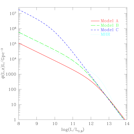
Figure 7: The Luminosity Function for our different models at $z=3.5$. Notice that all three models agree at the bright-end and only diverge due to the location of the break. For comparison, we also plot the LF from MHR.

The change in break luminosity for each model is illustrated in Figure 7, where we plot our results at $z=3.5$. (For comparison, we also show the MHR LF at the same redshift.) Note that in the limit that $L_{\rm min}\ll L_{*}\ll L(M_{B})$, our constraints follow the analytic relation

$$\log\left(\frac{L_{*}(z)}{\rm{L_{\odot,B}}}\right) \approx 12.2-1.72\log\hat{\varepsilon}^{Q}(z)-0.81(z-3)$$

$$\log\left(\frac{\phi_{*}(z)}{\rm{Gpc}^{-3}}\right) \approx 2.80+2.72\log\hat{\varepsilon}^{Q}(z)+0.81(z-3).$$ (18)

In practice we use these expressions as a starting point in our iterative solution for $L_{*}$ (and the implied value of $\phi_{*}$).

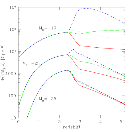
Figure 9: The evolution of the integrated number counts for the separate models, with lines defined the same as in Fig. 7.

A direct presentation of each Model LF at several discrete redshifts is shown in Figure 8. For the ionizing background of Model A, the faint-end of the LF is limited to virtually no evolution, while Model C allows considerable variation in the faint-end. The way in which these models evolve in terms of integrated number counts is illustrated in Fig. 9: for bright limiting magnitudes they show very similar evolution (by construction), while at faint magnitudes the evolution varies dramatically. Note that we have applied our emissivity constraints only for $z\geq 3$. For $z\leq 2.3$ we assume that the LF is fully defined by the 2dF results. Between these redshifts we have simply interpolated the values of $\phi_{*}$, $L_{*}$, and $\gamma_{b}$. The awkward line shapes from $z=2.3$ to 3 in Fig. 9 are due to this crude interpolation and should not be regarded as explicit predictions.

With our Model luminosity functions in hand, we are now in position to discuss our results in the context of several faint AGN searches. Before going on to do so, we briefly explore the degree to which our results depend on our input parameter assumptions.

5.1 Variations on Input Parameters

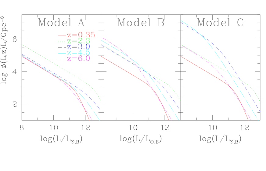
Figure 8: The Luminosity Function for different redshifts in our Models A, B, and C. The lines for $z=0.35$ and 2.3 are set by the 2dF data and, therefore, are common to all three models.

The evolution of $\phi_{*}$ and $L_{*}$ for our three ionizing background Models is illustrated in Figure 10, where we show our results using the parameter space introduced in conjunction with Figure 1 (§1). The solid, dashed, and short-dashed lines show how models A, B, and C evolve in this parameter space from $z=0$ to $6$, with triangles, squares, and pentagons marking specific redshifts: 3, 4, and 5, respectively. All of the models overlap on the diagonal line representing the observed 2dF LF evolution over the range $0<z<2.3$.

In order to estimate to what degree our input assumptions might affect our results, we have recalculated our constraints for a series of cases in which each of our inputs was varied (while all other parameters were kept fixed). The changes we explored were: varying $\gamma_{f}$ by $\pm 0.2$; varying $\eta_{\nu}$ by $\pm 40\%$; letting $\gamma_{b}=2.87$ (rather than our fiducial $\gamma_{b}=2.58$); allowing for non-zero cloud reemission of $\hat{\varepsilon}^{R}=0.4\hat{\varepsilon}^{Q}$ (see §4.2); and incorporating an IGM model with more absorption at high-redshift (as advocated by Fardal et al. (1998), see Appendix). We used this suite of cases to estimate plausible uncertainties in our model LFs at each redshift, and utilize these uncertainties in the next subsections. The error bars on the different redshift points in Figure 10 represent the largest changes in $\phi_{*}$ and $L_{*}$ we observed at each redshift for the changes described above. As can be seen from the figure, the primary changes are due to the adopted Model backgrounds, with variations on input parameters giving less important, although noticeable changes in the characteristic LF scales.

Probably the most straightforward change we observe comes from from varying $\eta_{\nu}$. Increasing (decreasing) $\eta_{\nu}$ requires fewer (more) faint AGN to reproduce the same ionizing background. Obtaining fewer AGN requires an increase in $L_{*}$ with a corresponding decrease in $\phi_{*}$ because the two parameters are constrained by the SDSS normalization: $\phi_{*}\propto L_{*}^{1-\gamma_{b}}$ (recall Fig. 1). For our $\pm 40\%$ variation in $\eta_{\nu}$, the effect on $\phi_{*}$ is about a factor of 2 , while $L_{*}$ varies by about 50%. Adding IGM reemission acts in the same way as increasing the value of $\eta_{\nu}$. In going from no reemission to $\hat{\varepsilon}^{R}=0.4\hat{\varepsilon}^{Q}$, $L_{*}$ increases by a factor of $\sim 2$, and $\phi_{*}$ decreases by a factor of $\sim 3$. Employing a model with more attenuation at high redshift (Fardal et al. 1998, Appendix) requires more AGN to match a given ionizing rate. The effect is most prominent in Model A for $z\gtrsim 4$. It increases $\phi_{*}$ by nearly a factor of 6.

Model	$\gamma_{f}$	$M_{B}^{*}(z=3,4,5)$	$N_{HDF}$	$N_{Keck}$
A	1.38	-25.2, -24.1, -22.9	0.15	66.0
	1.78	-27.0, -25.7, -24.3	0.17	90.6
B	1.38	-23.7, -21.9, -20.4	0.79	219
	1.78	-25.2, -23.1, -21.4	0.67	231
C	1.38	-20.3, -18.4, -18.4	4.64	1990
	1.78	-21.2, -19.2, -19.2	3.55	1520

Table 2 – We recalculate each model with a higher and lower value of the faint-end slope. In comparison to our fiducial values in Table 1, the changes to the break magnitude are well-approximated by Eq. 19. Notice, however, that the faint counts (see §5.2.1 and §5.2.2) are not highly-dependent on the choice of $\gamma_{f}$.

We have no observational constraints on $\gamma_{f}$ at high redshift, so variations in this parameter are certainly important to explore. A simple approximation of the emissivity integral, along with the SDSS normalization, gives us the variation to our fiducial ($\gamma_{f}=1.58$) break magnitude:

$$M_{B}^{*}(\gamma_{f})-M_{B}^{*}(1.58)\approx 1.6-4.3\log\left(\frac{2.58-\gamma_{f}}{2-\gamma_{f}}\right).$$ (19)

By iterating over the relevant equations, we obtain more precise estimates, which we list in Table 2 for $\gamma_{f}=1.38,1.78$ in each of our models. A flatter (steeper) faint-end slope requires more (less) AGN at “medium” luminosities to match a given background. This alteration is one of the dominant variations on Model A, since the break here is very near to the limits from the SDSS constraint (Eq. 2), and thereby the corrections to Eq. 19 are somewhat larger. In fact, at $z\sim 3$, a steeper $\gamma_{f}$ would make $M_{B}^{*}<-26$. A break at such a large absolute magnitude would presumably have been detected by WHO94 and SSG. Indeed, if current indications are correct and $M_{B}^{*}>-26$, then our fiducial Model A is close to being a minimum allowable LF. This possibility will be examined further in §6.

One last parameter that we give special attention to is $\gamma_{b}$. The SDSS value of 2.58 is quite a bit smaller than in previous determinations. Similar to the case of $\gamma_{f}$ for Model A, taking the steeper value of 2.87 from SSG has a relatively large effect on Models B and C (recall Fig. 1). In Model C the effect is nearly an order of magnitude in $L_{*}$. We plot this in Fig. 10 with a separate (dotted) error bar, although it is only visible above the (solid) error bar in cases where it exceeds all other uncertainties. Note that since the median redshifts of SSG and SDSS are, respectively, $\sim 3.3$ and $\sim 4$, it may be that $\gamma_{b}$ is evolving over these epochs.

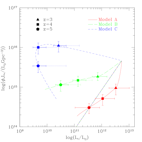
Figure 10: Solutions to the emissivity constrained models for $0<z<6$. The straight diagonal line is from the 2dF LF ($0<z<2.3$), which we force all of our models to agree with. The solid error bars come from varying parameters in the theory (see text). The dotted line error bars are specifically from taking the SSG value for $\gamma_{b}$.

5.2 Faint Surveys

There are several observations (either planned or completed) that are relevant to faint magnitude AGN. The counts obtained for the deeper, smaller fields that have been done so far are not as statistically significant as those based on large, shallow surveys we used to normalize our Model LF’s at the bright-end. However these fainter surveys do provide a useful consistency test for our Models, and forthcoming surveys for faint AGN will offer further tests of our input assumptions about the ionizing background. In this section we briefly investigate several surveys in light of our Model expectations and also predict what AGN counts might be seen by future observational programs.

5.2.1 Hubble Deep Field

The Hubble Deep Field is approximately 2.3 by 2.3 $\rm{arcmin}^{2}$. Looking only at unresolved sources, Conti et al. (1999) claim that there are no $z>3.5$ QSO candidates in the HDF down to estimated completeness limits of $\rm{B}_{450}\simeq 27,0$, $\rm{V}_{606}\simeq 27.0$, $\rm{I}_{814}\simeq 26.0$. The Conti et al. results are consistent with a similar HDF search by Elson, Santiago, & Gilmore (1996). Conservatively, we will assume that this implies an upper bound of 3 AGN per HDF field. For Poisson statistics, this corresponds to $5\%$ probability of seeing zero AGN. At slightly fainter magnitudes, Jarvis & MacAlpine (1998) take resolved sources in the HDF and select those with nuclei having the expected AGN colors. In the magnitude range $\rm{V}_{606}\sim 27.0-28.5$, for $z>3.5$, they find 12 candidates, but they make it clear this is an upper limit. We illustrate the observational bounds along with our three model expectations in Figure 11. Interestingly, there is one high redshift ($z\approx 3.5$) QSO seen by Chandra in the HDF (CXOHDFN J123639.5+621230.2, see Hornschemeier et al. 2001; Brandt et al. 2001). This object is not selected by either Jarvis & MacAlpine (1998) or Conti et al. (1999), even though it has $R=24.3$.

Using the Conti et al. limits ($\rm{V}_{606}<27.0$, $z>3.5$), we have calculated what each of our Models would have expected in the same field. These values are listed under $N_{HDF}$ in Table 1, along with an uncertainty calculated by the same variation of input parameters discussed in the previous section. Model C predicts too many QSOs. Even allowing $\gamma_{b}$ to be flatter than the SDSS value cannot reduce the expected value below $\sim 3$ per field. We discuss the implications of this in §6.

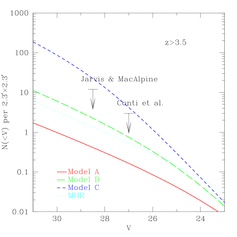
Figure 11: Number counts in the Hubble Deep Field for $z>3.5$. Shown are the predictions from our three models, as well as the upper limits from two searches for QSO candidates in the HDF.

5.2.2 Keck QSOs

Unlike most other surveys, which have targeted QSOs by their strong UV emission, Steidel and collaborators have only taken spectra of objects with strong continuum breaks at the rest-frame Lyman limit. Their technique was designed to find high-$z$ galaxies, which have an intrinsically softer spectrum at the Lyman continuum. Type I QSOs have much harder continua, so they would be generically missed by the Lyman-break selection technique. However an estimated $\sim 60\%$ of the lines of sight to $z\sim 3$ QSOs should have a foreground Lyman limit system at high enough redshift to create an “artificial” break. These are the AGN that get targeted for spectroscopic identification. Steidel et al. (2002) identified 13 type I QSOs between redshifts of 2.7 and 3.3 down to $\mathcal{R}=25.5$. Based on the size of their field and a rough estimate of their incompleteness, the implied number density of type I AGN is approximately $190$ per square degree.

We have compiled the expected number per square degree in each of our Models in Table 1 (with uncertainties determined as before). Again, Model C seems to over-predict (dramatically) the number of high-$z$ QSOs, while Model B, is consistent, at least within reasonable uncertainty. Interestingly, the LF motivated by the Steidel group’s own estimate for the stellar escape fraction (Model A) seems to under predict the expected QSO abundance by a factor of $\sim 2$. We discuss this in the next section.

Also detected in the same survey were 16 narrow lined, type II QSOs. These locally absorbed objects are quite important to the X-ray and, perhaps, IR backgrounds, but they are likely very weak emitters at ionizing frequencies, and therefore do not directly relate to the constraints we have set up. We will also address this population in §6.

5.2.3 Future Surveys

There are a number of future and ongoing surveys that plan to fill in the faint high redshift portion of the AGN LF. The Big Faint Quasar Survey (Hall 2001) will presumably probe the LF for $-26.5<M_{B}<-23.5$, for $z>3.5$. This is below the luminosity range of SDSS. Hall predicts that this survey (for $R<23.5$ and $7\rm{deg}^{2}$) will find $\sim 120$ quasars for $3.5<z<4$, and $\sim 40$ for $4<z<5$. While Model A with a substantial stellar contribution would predict fewer detections than this, Models B and C with AGN-dominated backgrounds expect 2-3 times as many QSOs.

The Space Infra-Red Telescope Facility (SIRTF) is proposed to have 1$\mu$Jy sensitivity, and the Next Generation Space Telescope (NGST) is proposed to have 1nJy sensitivity between 1 and 3.5$\mu$m. Although selecting high redshift QSOs in the Infra-Red may not be straightforward (see Warren & Hewett 2002), it is worthwhile to work out our theoretical predictions at these detection thresholds. These are shown in Figure 12.

Since all of our Models drop off steadily for $z>5$, the number counts illustrated in Figure 12 are dominated by the $z\sim 5$ QSOs. At this redshift for our chosen SED and cosmology, the proposed flux limits of SIRTF (NGST) would correspond to AGN with $L\simeq 10^{11}L_{\odot}$ ($10^{8}L_{\odot}$). We can compare our results to those of Haiman & Loeb (1998), who used a model based on CDM structure formation to predict that SIRTF would observe on the order of a few $z>5$ AGN, while NGST would see approximately $10^{3.5}$. A close examination of Haiman & Loeb’s differential LF (their Fig. 5) at $L\simeq 10^{11}L_{\odot,B}$ shows that it is an order of magnitude higher than the simplest extrapolation of the SDSS results. This explains why their SIRTF prediction is more than an order of magnitude higher than any of our predictions. So too, their NGST estimates are a factor of ten to a hundred above any of our estimates. However, this appears to be due to the fact that their LF is practically constant for $L<10^{10}L_{\odot}$ and $z>5$.

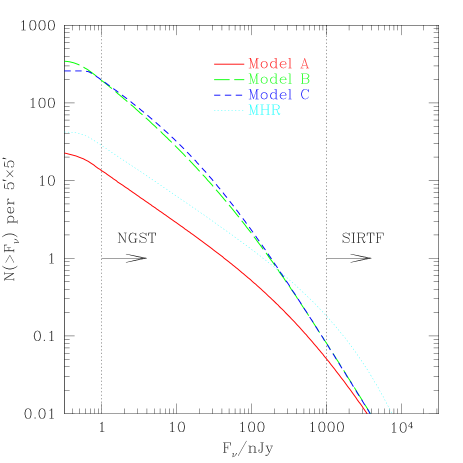
Figure 12: Predicted number counts in the $1-3.5\mu\rm{m}$ band for $z>5$ for our three models, as well as for MHR. The vertical lines are the proposed flux limits for future space telescopes.

6 Implications

In addition to direct constraints on the nature of the faint-AGN LF, our results have some interesting implications for the nature of ionizing sources as well as some typical characteristics of AGN themselves.

6.1 Ionizing Sources

Our joint analysis of the ionizing rate and faint AGN counts provides a potentially useful avenue for exploring the contribution of stars and AGN to the ionizing background. We showed in §5 that faint surveys do not find the number of QSOs that would be expected if all of the proximity-effect-derived background is coming only from AGN (Model C). Conversely, a model that reproduces the (lower) ionizing background intensity favored by the flux decrement technique under-predicts the faint counts unless the stellar contribution is limited (Model B). In this subsection we attempt to place more quantitative limits on the stellar contribution implied by the two competing background intensity measurements.

For each ionizing background measurement, we have calculated the expected number of Keck and HDF counts for several values of the escape fraction (§4.1). The results are shown in Figure 13, with the different symbol types reflecting different background assumptions: the squares represent a standard proximity effect background (Fardal et al. 1998) and the circles correspond to an assumed flux decrement background. In order to be conservative, we also include results for a background that matches the lower limit on the proximity effect rate taken from Scott et al. (2002) (triangles), with $\Gamma_{-12}\simeq 1.0$ over the range $1.7\lesssim z\lesssim 4.1$. Solid symbols include no IGM reemission and open symbols include $40\%$ cloud reemission. The horizontal dashed lines indicate the upper limit from the HDF search (upper panel) and observed AGN per square degree seen in the Keck fields (lower panel).

By examining Figure 13 we see that even with (the unphysically large value) $f_{\rm esc}=1$, the standard proximity effect background yields far too many Keck QSOs. A contribution from IGM reemission (§4.2) does little to lessen the discrepancy. The lower bound on the proximity effect from Scott et al. provides more reasonable numbers, but does require a significant stellar component, $f_{\rm esc}\lower 0.43057pt\hbox{\hbox to0.0pt{\raise 2.58334pt\hbox{\hskip 1.29167pt{{$\scriptscriptstyle>$}}}\hss} \kern-1.72218pt{{$\scriptscriptstyle\sim$}}}20\%$, even if we allow for a large amount of reemission. The flux-decrement-derived background, on the other hand, is not compatible with much stellar contribution: $f_{\rm esc}\lower 0.43057pt\hbox{\hbox to0.0pt{\raise 2.58334pt\hbox{\hskip 1.29167pt{{$\scriptscriptstyle<$}}}\hss} \kern-1.72218pt{{$\scriptscriptstyle\sim$}}}5\%$ is required in order to reproduce the Keck counts.

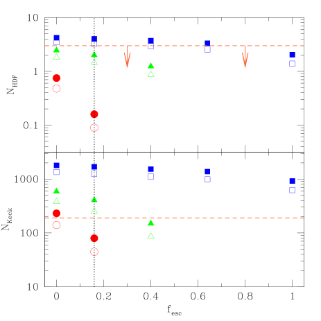
Figure 13: The expected number counts in the HDF (top) and Keck (bottom) surveys as a function of the escape fraction. The upper bound on the HDF and the observed number from Steidel et al. (2002) are plotted as dashed horizontal lines. The squares are for an ionizing background from the proximity effect (as parameterized by Fardal et al. 1998); the triangles are from the lower bound on the proximity effect from Scott et al. (2000); and the circles are from the flux decrement measurement of M&M-E. The open/solid points are with/without the contribution from cloud reemission ($\hat{\varepsilon}^{R}=0.4\hat{\varepsilon}^{Q}$). Note that we do not plot points at high escape fraction for the flux decrement (and for the lower bound on the proximity effect, as well), since the resulting LF breaks would contradict observations (see §5.1).

An additional way to examine the question of stellar escape fraction involves using the He Ly$\alpha$ forest to limit the relative amount of ionizing radiation from stars and AGN. Stars, unlike AGN, do not have much emission that extends to the helium Lyman continuum. This means that a stellar-dominated background should have a smaller relative fraction of fully ionized helium. At $z\sim 2.5$, the implied optical depth to He ii absorption is low enough that the background at these redshifts should be QSO-dominated (Davidson et al. 1996). But at slightly higher redshifts, Heap et al. (2000) appear to detect a Gunn-Peterson trough blueward of helium Ly$\alpha$ in the spectra of Q0302-003. They conclude that the ratio of hydrogen to helium ionization rates rises abruptly at $z\approx 3$ to $\Gamma_{\rm{HI}}/\Gamma_{\rm{HeII}}\simeq 800$, suggesting that a soft stellar contribution is beginning to dominate the hard ionizing spectrum of AGN at this epoch. This kind of rapid hardening of the background at $z\sim 3$ is supported by the analysis of Songaila (1998) of the Si iv/C iv ratio in the IGM. Although we do not model the propagation of helium ionizing photons in a very sophisticated way (see Appendix), we show in Figure 14 that Model A reproduces the reported evolution of $\Gamma_{\rm{HI}}/\Gamma_{\rm{HeII}}$ in a qualitative way. A more careful analysis of this phenomena will likely have to include the concomitant reionization of He ii (see Theuns et al. 2001). Recently, Sokasian, Abel, &. Hernquist (2002) have used observed opacities of HI and HeII to conclude that stars and AGN must contribute roughly equally to the ionizing background at $z\sim 3$. Theuns et al. (2002) and Bernardi et al. (2002) argue that the evolution of the flux decrement distribution studied via a sample of SDSS quasars points to HeII reionization at $z\simeq 3-4$.

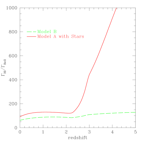
Figure 14: The softness parameter, $\Gamma_{\rm{HI}}/\Gamma_{\rm{HeII}}$, for Model B (QSOs only) and Model A (stars and QSOs). The rapid rise at $z\sim 3$ for Model A is qualitatively similar to that reported by Heap et al. (2000).

6.2 AGN Characteristics

In addition to quantifying our expectations for AGN counts in the presence of different ionizing backgrounds, our results have implications for the emission efficiency and lifetimes of AGN.

As discussed in §1, AGN activity is likely driven by accretion onto super-massive black holes. Under this assumption, the present-day density of black holes is related to the integrated AGN emissivity over the history of the universe, modulo the AGN efficiency (see Soltan 1982; Chokshi & Turner 1992; Haehnelt, Natarajan & Rees 1998). Because our models provide estimates of the maximum AGN emissivity out to high redshifts, we can convolve our results with an estimate of the density of black holes today in order to determine an implied efficiency.

Specifically the relic black hole density $\rho_{\bullet}$ is related to the integrated QSO energy density by $\rho_{Q}=\epsilon\rho_{\bullet}$, where $\epsilon\equiv L_{bol}/\dot{M}c^{2}$ is the QSO efficiency of converting mass into energy. The total energy output of QSOs can be obtained by integrating the emissivity over the history of the universe. If we define $\varepsilon_{B}(z)=\nu_{B}\varepsilon_{B}(\nu_{B},z)$ and $\nu_{B}=c/4400$Å, then we can write

$$\rho_{Q}=\frac{L_{bol}}{\nu_{B}L_{\nu}(\nu_{B})}\int\frac{dt}{dz}dz\cdot\varepsilon_{B}(z).$$ (20)

Because we are interested in the total energy output, we have applied a bolometric correction: $L_{bol}/\nu_{B}L_{\nu}(\nu_{B})=11.8$ (Elvis et al. 1994). We plot the B band emissivity for our three models in Figure 15. For $z<2.3$ we have used the 2dF LF fit from Boyle et al. (2000) to determine the emissivity, and between $z=2.3$ and 3, we linearly interpolate from the 2dF fit to our high redshift constraints. When we integrate from $z=0$ to 6, we find that Models A, B, and C give $\rho_{Q}=1.38,1.57,$ and $2.81$ respectively, in units of $10^{4}\rm{M_{\odot}Mpc^{-3}}$. The low-$z$ LF from the 2dF alone gives $\rho_{Q}(z\leq 2.3)=1.12$ in the same units. Thus a large fraction of the energy output from AGN seems to have occurred at late times even for our most extreme Model (C), and more than half for Models A and B .

The present day density in black holes can be estimated by assuming a typical black hole mass to spheroid mass ratio, $M_{\bullet}/M_{sp}$, and combining it with a local determination for the mass fraction in spheroids $\Omega_{sp}$. Adopting the fiducial value of $M_{\bullet}/M_{sp}=0.13\%$ (Merritt & Ferrarese 2001; McLure & Dunlop 2002; van der Marel 1999) and $\Omega_{sp}=0.002h^{-1}$ (Fukugita et al. 1998), we obtain

$$\rho_{\bullet}=5.0\times 10^{5}\left(\frac{M_{\bullet}/M_{sp}}{0.0013}\right)\left(\frac{\Omega_{sp}}{0.002h^{-1}}\right)\left(\frac{h}{0.7}\right)\rm{M_{\odot}Mpc^{-3}}.$$ (21)

Salucci et al. (1999) obtained a similar value ($8.2h^{2}\times 10^{5}\rm{M_{\odot}Mpc^{-3}}$) by convolving a distribution of $M_{\bullet}/M_{sp}$ values with an estimate of the spheroid mass function (see also Yu & Tremaine 2002). Adopting $\rho_{\bullet}=5.0\times 10^{5}\rm{M_{\odot}Mpc^{-3}}$, we obtain $\epsilon=\rho_{Q}/\rho_{\bullet}=0.028,0.032,$ and $0.056$ for models A, B, and C respectively.

Note that although these are in principle maximum efficiencies, based on maximum allowable AGN emissivities (because we have ignored reemission), they are significantly smaller than the often-adopted value of $\sim 0.1$. In addition, our derived efficiencies are significantly smaller than those obtained using the hard X-ray emissivity (Fabian & Iwasawa 1999; Salucci et al. 1999; Elvis et al. 2002). One possible explanation for this discrepancy is the existence of a large population of obscured AGN. If AGN efficiencies are typically $\lower 0.43057pt\hbox{\hbox to0.0pt{\raise 2.58334pt\hbox{\hskip 1.29167pt{{$\scriptscriptstyle>$}}}\hss} \kern-1.72218pt{{$\scriptscriptstyle\sim$}}}10\%$ (e.g. Elvis et al. 2002), then our results require that $\lower 0.43057pt\hbox{\hbox to0.0pt{\raise 2.58334pt\hbox{\hskip 1.29167pt{{$\scriptscriptstyle>$}}}\hss} \kern-1.72218pt{{$\scriptscriptstyle\sim$}}}~{}50-70\%$ of AGN are significantly obscured in the UV and optical. Interestingly, this result is similar to that obtained by synthesis modelers, $\sim 75-90\%$, based on the shape of the X-ray background spectrum (Comastri et al. 1995; Gilli et al. 2000) .

We have not considered type 2 AGN in our analysis simply because the implied absorption would mean they are not strong ionizing sources. But unification models assume that the type 2 population is not separate from the type 1s, but merely the result of an orientation effect. This would imply a non-trivial mapping between the mass function of supermassive black holes and the optical luminosity function. Therefore, to study the accretion history of the universe, it would seem to be more straightforward to use bands less affected by obscuration (see Marconi & Salvati 2001; Barger et al. 2001). Unfortunately, the X-ray LF at high redshift is limited statistically (Miyaji et al. 2000), and the AGN activity in many IR sources is still a matter of debate (see Lawrence 2001; Fadda et al. 2002). At high redshift, the best limits on the shape and evolution of the AGN LF still come from the optical/UV.

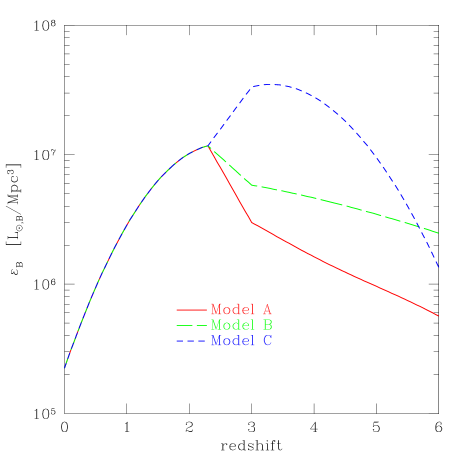
Figure 15: The emissivity in the B band. At low redshift we simply take the fit from 2dF. For $z>3$, we plot our three models with a simple linear interpolation to the 2dF limit of $z=2.3$. We have adopted units such that one $\rm{L_{\odot,B}}$ corresponds to $2.11\times 10^{33}\rm{erg/s}$ (see SSG).

Another constraint related to the local number density of black holes concerns the fraction of supermassive black holes that are active at any time, $f_{\rm on}(z)$. This can be related to a typical AGN lifetime, $t_{agn}$, which we define, via $f_{\rm on}(z)=t_{agn}(z)/t_{H}(z)$, to be the time that a typical black hole is active over the course of a Hubble time. For simplicity, let us assume that every AGN shines at a fixed fraction of the Eddington luminosity: $L=L_{\lambda}\equiv\lambda L_{Edd}$, where $L_{Edd}\approx 6\times 10^{3}(M_{\bullet}/\rm{M_{\odot}})\rm{L_{\odot,B}}$. With this assumption, we write $f_{\rm on}$ (averaged over luminosity) as

$$f_{\rm on}(z)\equiv\frac{\Phi(>L_{\lambda},z)}{N(>M_{\bullet},z)}\geq\frac{\Phi(>L_{\lambda},z)}{N(>M_{\bullet},z=0)}.$$ (22)

The inequality comes from the assumption that a given black hole’s mass only grows with time and that the black hole mass function is a decreasing function of mass. One possible caveat to this inequality is that black hole merging could (but not necessarily) reduce the number of low-mass black holes with time. In this case, the above inequality would break down. However, in the case of halos of mass $\sim 10^{10}M_{\odot}$ (corresponding to black holes of $\sim 10^{6}M_{\odot}$), the number density does not decrease substantially from $z\sim 5$ to the present. This is because most merging occurs in high-mass-ratio events.

So assuming Expression 22 is valid, we can take for the denominator the results of Salucci et al. (1999), who estimate that $N(>M_{\bullet},z=0)\simeq 10^{-2}\rm{Mpc}^{-3}$ for $M_{\bullet}=10^{6}{\rm M_{\odot}}$. Given $\lambda$, this number allows us to determine the implied lower limits on $f_{\rm on}(z)$ for each of our Models. We plot these limits in Figure 16 for $\lambda=1.0$ ($L_{\lambda}=6\times 10^{9}\rm{L_{\odot,B}}$) and $\lambda=0.05$ ($L_{\lambda}=3\times 10^{8}\rm{L_{\odot,B}}$). Fortunately, none of our models result in the unphysical $f_{\rm on}>1$. But for the corresponding lifetime limits, Model C requires very long-lived AGN at high-$z$: $t_{agn}\lower 0.43057pt\hbox{\hbox to0.0pt{\raise 2.58334pt\hbox{\hskip 1.29167pt{{$\scriptscriptstyle>$}}}\hss} \kern-1.72218pt{{$\scriptscriptstyle\sim$}}}10^{8}$yr, whereas Models A and B suggest lifetimes that are on the high-side of what is typically assumed: $t_{agn}\lower 0.43057pt\hbox{\hbox to0.0pt{\raise 2.58334pt\hbox{\hskip 1.29167pt{{$\scriptscriptstyle>$}}}\hss} \kern-1.72218pt{{$\scriptscriptstyle\sim$}}}10^{7}$yr. If estimates of the AGN lifetime from other lines of reasoning can be obtained (e.g. Martini & Weinberg 2001; Haiman & Hui 2001), then this sort of analysis may be capable of restricting theories on the history of black hole accretion (see Ciotti et al. 2001).

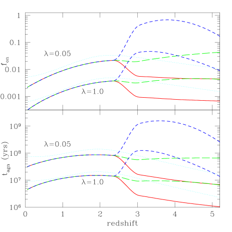
Figure 16: Top- lower bounds on the fraction of $10^{6}{\rm M_{\odot}}$ black holes that are active at any redshift; bottom- implied lower bounds on typical AGN lifetimes (see text for a description). We plot two assumptions for the ratio of AGN luminosities to the Eddington luminosity: $\lambda\equiv L/L_{Edd}$ equal to 0.05 (upper set of curves) and 1.0 (lower). Our three models are represented, along with the model of MHR for comparison. The lines are defined as in Figure 7.

7 Summary and Conclusions

In this paper, we have explored the implied evolution of the faint AGN luminosity function using three different models for the ionizing background from $3\lower 0.43057pt\hbox{\hbox to0.0pt{\raise 2.58334pt\hbox{\hskip 1.29167pt{{$\scriptscriptstyle<$}}}\hss} \kern-1.72218pt{{$\scriptscriptstyle\sim$}}}z\lower 0.43057pt\hbox{\hbox to0.0pt{\raise 2.58334pt\hbox{\hskip 1.29167pt{{$\scriptscriptstyle<$}}}\hss} \kern-1.72218pt{{$\scriptscriptstyle\sim$}}}6$. Our LFs are derived by matching the implied faint-end emissivity. Unfortunately, the value of the ionizing background rate is not universally agreed upon. Measurements obtained using the proximity effect generally give larger values than those based on the flux decrement distribution.

Although the current data on faint AGN come from small-field searches with only modest statistical accuracy, we have used them to obtain rough evaluations of our Models. If AGN were producing a background at the level measured by the proximity effect technique, then significantly more would have been seen in the HDF and LBG fields. For typical proximity effect values of the background, even an escape fraction of unity would require more than three times the number of AGN observed in the Keck fields. We were able to obtain modest agreement only by taking the lowest bounds on the proximity effect measurements and by including a high galactic escape fraction: $f_{\rm esc}\lower 0.43057pt\hbox{\hbox to0.0pt{\raise 2.58334pt\hbox{\hskip 1.29167pt{{$\scriptscriptstyle>$}}}\hss} \kern-1.72218pt{{$\scriptscriptstyle\sim$}}}20\%$. Conversely, if the flux decrement rate is adopted, there is little room for a significant stellar component, and $f_{\rm esc}\lower 0.43057pt\hbox{\hbox to0.0pt{\raise 2.58334pt\hbox{\hskip 1.29167pt{{$\scriptscriptstyle<$}}}\hss} \kern-1.72218pt{{$\scriptscriptstyle\sim$}}}5\%$ is required to match the faint AGN counts. Future AGN searches and developments in our ability to measure the background intensity will be useful for further constraining the stellar contribution to the ionizing background at high-$z$.

We used our derived luminosity functions and local determinations of the black hole relic density to determine the typical AGN efficiency of converting mass to light. Although many previous estimates based on X-ray counts have obtained $\epsilon\lower 0.43057pt\hbox{\hbox to0.0pt{\raise 2.58334pt\hbox{\hskip 1.29167pt{{$\scriptscriptstyle>$}}}\hss} \kern-1.72218pt{{$\scriptscriptstyle\sim$}}}0.1$ (e.g. Elvis et al. 2002), we find significantly lower values $\epsilon\simeq 0.028-0.056$, suggesting that more than half of all AGN are obscured in the UV/optical. Alternatively, lower than expected values of $\epsilon$ may be derived if much of a black hole’s mass is set by a massive “seed” before the onset of its active phase. A joint analysis of UV-background measurements, optical counts, and X-ray observations would likely resolve this issue.

A similar analysis allows us to limit the fraction of black holes that could have been active at any redshift. For our models that are most consistent with faint AGN counts, we get $f_{\rm on}\lower 0.43057pt\hbox{\hbox to0.0pt{\raise 2.58334pt\hbox{\hskip 1.29167pt{{$\scriptscriptstyle>$}}}\hss} \kern-1.72218pt{{$\scriptscriptstyle\sim$}}}0.5\%$ at $z\sim 2.5$. We can interpret this in terms of a lower limit on the average AGN lifetime: $t_{agn}\lower 0.43057pt\hbox{\hbox to0.0pt{\raise 2.58334pt\hbox{\hskip 1.29167pt{{$\scriptscriptstyle>$}}}\hss} \kern-1.72218pt{{$\scriptscriptstyle\sim$}}}10^{7}\rm{yrs}$. For comparison, an AGN luminosity function that matches the proximity effect background (but over-produces the faint counts) requires $f_{\rm on}\lower 0.43057pt\hbox{\hbox to0.0pt{\raise 2.58334pt\hbox{\hskip 1.29167pt{{$\scriptscriptstyle>$}}}\hss} \kern-1.72218pt{{$\scriptscriptstyle\sim$}}}5\%$ and $t_{agn}\lower 0.43057pt\hbox{\hbox to0.0pt{\raise 2.58334pt\hbox{\hskip 1.29167pt{{$\scriptscriptstyle>$}}}\hss} \kern-1.72218pt{{$\scriptscriptstyle\sim$}}}10^{8}\rm{yrs}$. Note that these numbers are firm lower limits because we assume that there are no obscured AGN. If a fraction of AGN were obscured in the optical, then these limits would be increased by the inverse of the same fraction.

Finally, we conclude with some remarks about CDM-based theories of AGN formation and how they might be constrained. Usually cosmological models of this kind rely on simple mappings between dark halo masses and AGN luminosities, but a fundamental unknown concerns the amount of feedback that takes place (e.g. Haehnelt & Rees 1993, Haiman & Loeb 1998). We point out that one potentially worrisome difficulty for models with very little feedback arises from direct observations of the AGN LF at bright luminosities. Specifically, the bright-end slope measured by the SDSS at high redshift is even flatter than that measured by the 2dF at low redshift. This is the opposite of what is expected if the AGN LF maps simply to the halo mass accretion rate function (see, e.g., Haiman & Loeb 1998). Therefore the SDSS+2dF results alone seem to suggest that some feedback is needed for bright to intermediate luminosity AGN.

Another question is whether any (additional) feedback might be needed in low-mass/ low-luminosity objects in order to explain the observed ionizing background rate at high-$z$. As discussed above, our Models A and B span what we believe to be the range allowed by the ionizing rate measurements. Model B corresponds to the case where AGN dominate the background, and, interestingly, its evolution is very reminiscent to that of the halo mass function in CDM: faint AGN are numerous at early times, but their numbers fall-off slowly at late times (see Figure 8). It would seem that if AGN do dominate the ionizing background, then CDM-models would require no additional feedback on low mass scales (relative to what might already be required at the high-mass end in order to match the SDSS results.)

If instead stars contribute with an escape fraction consistent with the Steidel et al. (2002) report (Model A), then many fewer AGN are permitted, and CDM-based models would need to be adjusted further in order to additionally suppress the formation of low-luminosity AGN. Both Haiman, Madau & Loeb (1999) and Kauffmann & Haehnelt (2000) presented models with this kind of luminosity-dependent feedback, but it is unclear if, as presented, these models would be able to reproduce both the ionizing rate (with an allowance for stars) and the faint AGN counts in the HDF and LBG fields. It would be interesting to see such a comparison. The model of Kauffmann & Haehnelt (2000) is ideally suited for this test because it predicts the joint population of galaxies and AGN in a self-consistent manner.

It is becoming increasingly clear that galaxy formation, AGN activity, and the resulting ionizing background are intimately connected and take part in an important feedback loop (Gebhardt et al. 2000a; Ferrarese & Merritt 2000; Kauffmann & Haehnelt 2000; Bullock, Kravtsov, & Weinberg 2000; Benson et al. 2002; Somerville 2002). For this reason the need is high for self-consistent models that treat all of these processes together, as is the need for additional observational constraints on models of this kind. The limits presented here provide one small step in this direction, but if some agreement can be reached on measurements of the ionizing background emissivity, the resulting constraints would prove remarkably important for piecing together the story of cosmological structure formation.

The following comes primarily from MHR, but see also Fardal et al. (1998). The attenuation due to photoelectric absorption can be modelled by a distribution of discrete absorbers (or “clouds”):

$$\tau_{eff}(\nu,z,\bar{z})=\int^{\bar{z}}_{z}dz^{\prime}\int^{\infty}_{0}dN_{\rm{HI}}\frac{\partial^{2}N}{\partial N_{\rm{HI}}\partial z^{\prime}}(1-e^{-\tau(\nu^{\prime})})$$ (1)

where $\nu^{\prime}=\nu\ (1+z^{\prime})/(1+z)$, and, for a given absorber, $N_{\rm{HI}}$ is the column density in neutral hydrogen. This distribution is usually parameterized as:

$$\frac{\partial^{2}N}{\partial N_{\rm{HI}}\partial z^{\prime}}=\frac{1}{N_{o}}\left(\frac{N_{\rm{HI}}}{N_{o}}\right)^{-\beta}(1+z^{\prime})^{\gamma}$$ (2)

If we assume that the distribution is smooth over redshift and column density, then we get an analytical expression for the effective optical depth. We assume $N_{o}=1.6\times 10^{15}\rm{cm}^{-2}$, $\beta=1.5$, $\gamma=2$, which MHR claim approximate more precise formulations. [In §5.1 we compare what our results would be using the corresponding model from Fardal et al. (1998): $N_{o}=3.27\times 10^{14}\rm{cm}^{-2}$, $\beta=1.5$, $\gamma=2.58$.] As for the attenuation in a particular cloud, we will consider only H i and He ii absorption:

$$\tau(\nu^{\prime})=N_{\rm{HI}}\sigma_{\rm{HI}}(\nu^{\prime})+N_{\rm{HeII}}\sigma_{\rm{HeII}}(\nu^{\prime})$$ (3)

The cross sections are zero below threshold ($\nu_{\rm{H}}=13.6$eV; $\nu_{\rm{HeII}}=54.4$eV), and above threshold are proportional to $\nu^{-3}$, with $\sigma_{\rm{H}}(\nu_{\rm{H}})=6.35\times 10^{-18}{\rm{cm}}^{2}$ and $\sigma_{\rm{HeII}}(\nu_{\rm{HeII}})=1.59\times 10^{-18}{\rm{cm}}^{2}$. These cross sections are separated far enough in frequency that we can consider the ionization state of hydrogen and helium separately. We can make the approximation that the relevant clouds are optically thin (see Haardt & Madau 1996; Fardal et al. 1998), so that:

$$\eta\equiv\frac{N_{\rm{HeII}}}{N_{\rm{HI}}}=0.45\frac{\Gamma_{\rm HI}}{\Gamma_{\rm HeII}}$$ (4)

This relation will not hold true in high column density clouds because of self-shielding effects, but these clouds are less abundant and therefore are less important to the effective attenuation. In any case, a more careful study of the helium ionization state should take into account the self-shielding and reemission in the IGM.

References

- Bajtlik, Duncan, & Ostriker (1988) Bajtlik, S., Duncan, R. C., & Ostriker, J. P. 1988, ApJ, 327, 570
- Barger et al. (2001) Barger, A. J., Cowie, L. L., Bautz, M. W., Brandt, W. N., Garmire, G. P., Hornschemeier, A. E., Ivison, R. J., & Owen, F. N. 2001, AJ, 122, 2177
- Barkana & Loeb (2000) Barkana, R. & Loeb, A. 2000, ApJ, 531, 613
- Bechtold (1994) Bechtold, J. 1994, ApJS, 91, 1
- Benson et al. (2002) Benson, A. J., Lacey, C. G., Baugh, C. M., Cole, S., & Frenk, C. S. 2002, MNRAS, 333, 156
- Bernardi et al. (2002) Bernardi, M., Sheth, R. K., Subbarao, M. et al. 2002, ApJ, submitted, astro-ph/0206293
- Bianchi, Cristiani, & Kim (2001) Bianchi, S., Cristiani, S., & Kim, T.-S. 2001, A&A, 376, 1
- Bland-Hawthorn & Maloney (2001) Bland-Hawthorn, J. & Maloney, P. R. 2001, ApJ, 550, L231
- Blandford & Narayan (1992) Blandford, R. D. & Narayan, R. 1992, ARA&A, 30, 311
- Boyle, Shanks, & Peterson (1988) Boyle, B. J., Shanks, T., & Peterson, B. A. 1988, MNRAS, 235, 935
- Boyle & Terlevich (1998) Boyle, B. J. & Terlevich, R. J. 1998, MNRAS, 293, L49
- Boyle et al. (2000) Boyle, B. J., Shanks, T., Croom, S. M., Smith, R. J., Miller, L., Loaring, N., & Heymans, C. 2000, MNRAS, 317, 1014
- Brandt et al. (2001) Brandt, W. N. et al. 2001, AJ, 122, 1
- Bullock, Kravtsov, & Weinberg (2000) Bullock, J. S., Kravtsov, A. V., & Weinberg, D. H. 2000, ApJ, 539, 517
- Bullock et al. (2002) Bullock, J. S., Somerville, R. S., Devriendt, J. E. G., & Primack, J. R. 2002, in preparation
- Burles & Tytler (1998) Burles, S. & Tytler, D. 1998, ApJ, 507, 732
- Canalizo & Stockton (2001) Canalizo, G. & Stockton, A. 2001, ApJ, 555, 719
- Carlberg (1990) Carlberg, R. G. 1990, ApJ, 350, 505
- Cattaneo, Haehnelt, & Rees (1999) Cattaneo, A., Haehnelt, M. G., & Rees, M. J. 1999, MNRAS, 308, 77
- Cavaliere, Perri, & Vittorini (1997) Cavaliere, A., Perri, M., & Vittorini, V. 1997, Memorie della Societa Astronomica Italiana, 68, 27
- Cen & McDonald (2002) Cen, R. & McDonald, P. 2002, ApJ, 570, 457
- Cen, Miralda-Escude, Ostriker, & Rauch (1994) Cen, R., Miralda-Escude, J., Ostriker, J. P., & Rauch, M. 1994, ApJ, 437, L9
- Chokshi & Turner (1992) Chokshi, A. & Turner, E. L. 1992, MNRAS, 259, 421
- Ciotti, Haiman, & Ostriker (2001) Ciotti, L., Haiman, Z., & Ostriker, J. P. 2001, 2 pages, to appear on ESO Astrophysics Symposia ”The Mass of Galaxies at Low and High Redshift”, R. Bender and A. Renzini, eds Preprint no. BAP12-2001-20-OAB., 12131
- Conti, Kennefick, Martini, & Osmer (1999) Conti, A., Kennefick, J. D., Martini, P., & Osmer, P. S. 1999, AJ, 117, 645
- Cooke, Espey, & Carswell (1997) Cooke, A. J., Espey, B., & Carswell, R. F. 1997, MNRAS, 284, 552
- Cristiani et al. (1995) Cristiani, S., D’Odorico, S., Fontana, A., Giallongo, E., & Savaglio, S. 1995, MNRAS, 273, 1016
- Dave, Hernquist, Weinberg, & Katz (1997) Davé, R., Hernquist, L., Weinberg, D. H., & Katz, N. 1997, ApJ, 477, 21
- (29) Davé, R. & Tripp, T.M. 2001, ApJ, 553, 528.
- Dawson et al. (2002) Dawson, S., Spinrad, H., Stern, D., Dey, A., van Breugel, W., de Vries, W., & Reuland, M. 2002, ApJ, 570, 92
- Deharveng et al. (2001) Deharveng, J.-M., Buat, V., Le Brun, V., Milliard, B., Kunth, D., Shull, J. M., & Gry, C. 2001, A&A, 375, 805
- Dickinson et al. (1998) Dickinson, M. et al. 1998, American Astronomical Society Meeting, 30, 1367
- Eisenstein & Loeb (1995) Eisenstein, D. J. & Loeb, A. 1995, ApJ, 443, 11
- Ellison et al. (2001) Ellison, S. L., Yan, L., Hook, I. M., Pettini, M., Wall, J. V., & Shaver, P. 2001, A&A, 379, 393
- Ellison et al. (2002) Ellison, S. L., Yan, L., Hook, I. M., Pettini, M., Wall, J. V., & Shaver, P. 2002, A&A, 383, 91
- Elson, Santiago, & Gilmore (1996) Elson, R. A. W., Santiago, B. X., & Gilmore, G. F. 1996, New Astronomy, 1, 1
- Elvis et al. (1994) Elvis, M. et al. 1994, ApJS, 95, 1
- Elvis, Risaliti, & Zamorani (2002) Elvis, M., Risaliti, G., & Zamorani, G. 2002, ApJ, 565, L75
- Efstathiou & Rees (1988) Efstathiou, G. & Rees, M. J. 1988, MNRAS, 230, 5P
- Fabian & Iwasawa (1999) Fabian, A. C. & Iwasawa, K. 1999, MNRAS, 303, L34
- Fadda et al. (2002) Fadda, D., Flores, H., Hasinger, G., Franceschini, A., Altieri, B., Cesarsky, C. J., Elbaz, D., & Ferrando, P. 2002, A&A, 383, 838
- Fall & Pei (1993) Fall, S. M. & Pei, Y. C. 1993, ApJ, 402, 479
- Fan et al. (2001) Fan, X. et al. 2001a, AJ, 121, 54
- Fan et al. (2001) Fan, X. et al. 2001b, AJ, 122, 2833
- Fan et al. (2002) Fan, X., Narayanan, V. K., Strauss, M. A., White, R. L., Becker, R. H., Pentericci, L., & Rix, H. 2002, AJ, 123, 1247
- Fardal, Giroux, & Shull (1998) Fardal, M. A., Giroux, M. L., & Shull, J. M. 1998, AJ, 115, 2206
- Ferguson & STIS HDF-UV Collaboration (2001) Ferguson, H. C. & STIS HDF-UV Collaboration 2001, American Astronomical Society Meeting, 198, 2003
- Fernandez-Soto, Barcons, Carballo, & Webb (1995) Fernandez-Soto, A., Barcons, X., Carballo, R., & Webb, J. K. 1995, MNRAS, 277, 235
- Ferrarese (2002) Ferrarese, L. 2002, astro-ph/0203469
- Ferrarese & Merritt (2000) Ferrarese, L. & Merritt, D. 2000, ApJ, 539, L9
- Ferrarese et al. (2001) Ferrarese, L., Pogge, R. W., Peterson, B. M., Merritt, D., Wandel, A., & Joseph, C. L. 2001, ApJ, 555, L79
- Franceschini, Hasinger, Miyaji, & Malquori (1999) Franceschini, A., Hasinger, G., Miyaji, T., & Malquori, D. 1999, MNRAS, 310, L5
- Fukugita, Hogan, & Peebles (1998) Fukugita, M., Hogan, C. J., & Peebles, P. J. E. 1998, ApJ, 503, 518
- Gebhardt et al. (2000) Gebhardt, K. et al. 2000a, ApJ, 539, L13
- Gebhardt et al. (2000) Gebhardt, K. et al. 2000b, ApJ, 543, L5
- Giallongo et al. (1996) Giallongo, E., Cristiani, S., D’Odorico, S., Fontana, A., & Savaglio, S. 1996, ApJ, 466, 46
- Giallongo, Cristiani, D’Odorico, & Fontana (2002) Giallongo, E., Cristiani, S., D’Odorico, S., & Fontana, A. 2002, ApJ, 568, L9
- Gilli, Salvati, & Hasinger (2001) Gilli, R., Salvati, M., & Hasinger, G. 2001, A&A, 366, 407
- Gnedin & Hamilton (2002) Gnedin, N. Y. & Hamilton, A. J. S. 2002, MNRAS, 334, 107
- Gunn & Peterson (1965) Gunn, J. E. & Peterson, B. A. 1965, ApJ, 142, 1633
- Haardt & Madau (1996) Haardt, F. & Madau, P. 1996, ApJ, 461, 20
- Haehnelt & Kauffmann (2001) Haehnelt, M. G. & Kauffmann, G. 2001, Black Holes in Binaries and Galactic Nuclei, 364
- Haehnelt, Madau, Kudritzki, & Haardt (2001) Haehnelt, M. G., Madau, P., Kudritzki, R., & Haardt, F. 2001, ApJ, 549, L151
- Haehnelt, Natarajan, & Rees (1998) Haehnelt, M. G., Natarajan, P., & Rees, M. J. 1998, MNRAS, 300, 817
- Haehnelt & Rees (1993) Haehnelt, M. G. & Rees, M. J. 1993, MNRAS, 263, 168
- Haiman & Hui (2001) Haiman, Z. & Hui, L. 2001, ApJ, 547, 27
- Haiman & Loeb (1998) Haiman, Z. & Loeb, A. 1998, ApJ, 503, 505
- Haiman & Loeb (1999) Haiman, Z. & Loeb, A. 1999, After the Dark Ages: When Galaxies were Young (the Universe at ). 9th Annual October Astrophysics Conference in Maryland held 12-14 October, 1998. College Park, Maryland. Edited by S. Holt and E. Smith. American Institute of Physics Press, 1999, p. 34., 34
- Haiman, Madau, & Loeb (1999) Haiman, Z., Madau, P., & Loeb, A. 1999, ApJ, 514, 535
- Hall (2001) Hall, P. B. 2001, ASP Conf. Ser. 232: The New Era of Wide Field Astronomy, 84
- Hartwick & Schade (1990) Hartwick, F. D. A. & Schade, D. 1990, ARA&A, 28, 437
- Hasinger (2002) Hasinger, G. 2002, astro-ph/0202430
- Heap et al. (2000) Heap, S. R., Williger, G. M., Smette, A., Hubeny, I., Sahu, M. S., Jenkins, E. B., Tripp, T. M., & Winkler, J. N. 2000, ApJ, 534, 69
- Heckman, Smith, Bothun, & Balick (1984) Heckman, T. M., Smith, E. P., Bothun, G. D., & Balick, B. 1984, BAAS, 16, 481
- Hernquist, Katz, Weinberg, & Jordi (1996) Hernquist, L., Katz, N., Weinberg, D. H., & Jordi, M. 1996, ApJ, 457, L51
- Hewett, Foltz, & Chaffee (1993) Hewett, P. C., Foltz, C. B., & Chaffee, F. H. 1993, ApJ, 406, L43
- Hook, Shaver, & McMahon (1998) Hook, I. M., Shaver, P. A., & McMahon, R. G. 1998, ASP Conf. Ser. 146: The Young Universe: Galaxy Formation and Evolution at Intermediate and High Redshift, 17
- Hornschemeier et al. (2001) Hornschemeier, A. E. et al. 2001, ApJ, 554, 742
- Hui, Haiman, Zaldarriaga, & Alexander (2002) Hui, L., Haiman, Z., Zaldarriaga, M., & Alexander, T. 2002, ApJ, 564, 525
- Hurwitz, Jelinsky, & Dixon (1997) Hurwitz, M., Jelinsky, P., & Dixon, W. V. D. 1997, ApJ, 481, L31
- Jarvis & MacAlpine (1998) Jarvis, R. M. & MacAlpine, G. M. 1998, AJ, 116, 2624
- Kauffmann & Haehnelt (2000) Kauffmann, G. & Haehnelt, M. 2000, MNRAS, 311, 576
- Kennefick, Djorgovski, & de Carvalho (1995) Kennefick, J. D., Djorgovski, S. G., & de Carvalho, R. R. 1995, AJ, 110, 2553 [KDC95]
- Koo & Kron (1988) Koo, D. C. & Kron, R. G. 1988, ApJ, 325, 92
- Koratkar & Blaes (1999) Koratkar, A. & Blaes, O. 1999, PASP, 111, 1
- Kormendy & Richstone (1995) Kormendy, J. & Richstone, D. 1995, ARA&A, 33, 581
- Koushiappas, Bullock, & Dekel (2002) Koushiappas, S. M., Bullock, J. S., & Dekel A. 2002, in preparation
- Kuhn, Elvis, Bechtold, & Elston (2001) Kuhn, O., Elvis, M., Bechtold, J., & Elston, R. 2001, ApJS, 136, 225
- Laor (1998) Laor, A. 1998, ApJ, 505, L83
- Lawrence (2001) Lawrence, A. 2001, The Promise of the Herschel Space Observatory. Eds. G.L. Pilbratt, J. Cernicharo, A.M. Heras, T. Prusti, & R. Harris. ESA-SP 460, p. 95
- Leitherer, Ferguson, Heckman, & Lowenthal (1995) Leitherer, C., Ferguson, H. C., Heckman, T. M., & Lowenthal, J. D. 1995, ApJ, 454, L19
- Levenson, Weaver, & Heckman (2001) Levenson, N. A., Weaver, K. A., & Heckman, T. M. 2001, ApJ, 550, 230
- Liske & Williger (2001) Liske, J. & Williger, G. M. 2001, MNRAS, 328, 653
- Loeb & Eisenstein (1995) Loeb, A. & Eisenstein, D. J. 1995, ApJ, 448, 17
- Londish, Boyle, & Schade (2000) Londish, D., Boyle, B. J., & Schade, D. J. 2000, MNRAS, 318, 411
- Lynden-Bell (1969) Lynden-Bell, D. 1969, Nature, 223, 690
- Madau (1992) Madau, P. 1992, ApJ, 389, L1
- Madau (1995) Madau, P. 1995, ApJ, 441, 18
- Madau, Haardt, & Rees (1999) Madau, P., Haardt, F., & Rees, M. J. 1999, ApJ, 514, 648 [MHR]
- Madau & Phinney (1996) Madau, P. & Phinney, E. S. 1996, ApJ, 456, 124
- Madau & Rees (2001) Madau, P. & Rees, M. J. 2001, ApJ, 551, L27
- Madau & Shull (1996) Madau, P. & Shull, J. M. 1996, ApJ, 457, 551
- Magorrian et al. (1998) Magorrian, J. et al. 1998, AJ, 115, 2285
- Marconi & Salvati (2001) Marconi, A. & Salvati, M. 2001, astro-ph/0110698
- Martini & Weinberg (2001) Martini, P. & Weinberg, D. H. 2001, ApJ, 547, 12
- Mathur (2000) Mathur, S. 2000, MNRAS, 314, L17
- McLure & Dunlop (2002) McLure, R. J. & Dunlop, J. S. 2002, MNRAS, 331, 795
- McDonald et al. (2000) McDonald, P., Miralda-Escudé, J., Rauch, M., Sargent, W. L. W., Barlow, T. A., Cen, R., & Ostriker, J. P. 2000, ApJ, 543, 1
- McDonald & Miralda-Escudé (2001) McDonald, P. & Miralda-Escudé, J. 2001, ApJ, 549, L11 [M&M-E]
- Miralda-Escude, Cen, Ostriker, & Rauch (1996) Miralda-Escude, J., Cen, R., Ostriker, J. P., & Rauch, M. 1996, ApJ, 471, 582
- Miralda-Escudé & Ostriker (1990) Miralda-Escudé, J. & Ostriker, J. P. 1990, ApJ, 350, 1
- Miyaji, Hasinger, & Schmidt (2000) Miyaji, T., Hasinger, G., & Schmidt, M. 2000, A&A, 353, 25
- Pascarelle, Lanzetta, Chen, & Webb (2001) Pascarelle, S. M., Lanzetta, K. M., Chen, H., & Webb, J. K. 2001, ApJ, 560, 101
- Pei (1995) Pei, Y. C. 1995a, ApJ, 438, 623
- Pei (1995) Pei, Y. C. 1995b, ApJ, 440, 485
- Poli et al. (2001) Poli, F., Menci, N., Giallongo, E., Fontana, A., Cristiani, S., & D’Odorico, S. 2001, ApJ, 551, L45
- Primack, Somerville, Bullock, & Devriendt (2001) Primack, J. R., Somerville, R. S., Bullock, J. S., & Devriendt, J. E. G. 2001, High Energy Gamma-Ray Astronomy, 463
- Randall & Sarazin (2001) Randall, S. W. & Sarazin, C. L. 2001, ApJ, 548, 60
- Rauch et al. (1997) Rauch, M. et al. 1997, ApJ, 489, 7
- Rees (1984) Rees, M. J. 1984, ARA&A, 22, 471
- Richstone et al. (1998) Richstone, D. et al. 1998, Nature, 395, A14
- Salpeter (1964) Salpeter, E. E. 1964, ApJ, 140, 796
- Salucci, Szuszkiewicz, Monaco, & Danese (1999) Salucci, P., Szuszkiewicz, E., Monaco, P., & Danese, L. 1999, MNRAS, 307, 637
- Sanders et al. (1988) Sanders, D. B., Soifer, B. T., Elias, J. H., Madore, B. F., Matthews, K., Neugebauer, G., & Scoville, N. Z. 1988, ApJ, 325, 74
- Sanders & Mirabel (1996) Sanders, D. B. & Mirabel, I. F. 1996, ARA&A, 34, 749
- Schmidt, Schneider, & Gunn (1995) Schmidt, M., Schneider, D. P., & Gunn, J. E. 1995, AJ, 110, 68 [SSG]
- Scott, Bechtold, Dobrzycki, & Kulkarni (2000) Scott, J., Bechtold, J., Dobrzycki, A., & Kulkarni, V. P. 2000, ApJS, 130, 67
- Sharp, McMahon, Irwin, & Hodgkin (2001) Sharp, R. G., McMahon, R. G., Irwin, M. J., & Hodgkin, S. T. 2001, MNRAS, 326, L45
- Shull et al. (1999) Shull, J. M., Roberts, D., Giroux, M. L., Penton, S. V., & Fardal, M. A. 1999, AJ, 118, 1450
- Sokasian et al. (2002) Sokasian, A., Abel, T., Hernquist, L. E. 2002, astro-ph/0206428
- Soltan (1982) Soltan, A. 1982, MNRAS, 200, 115
- Somerville (2002) Somerville, R. S. 2002, ApJ, 572, L23
- Somerville, Primack, & Faber (2001) Somerville, R. S., Primack, J. R., & Faber, S. M. 2001, MNRAS, 320, 504
- Songaila (1998) Songaila, A. 1998, AJ, 115, 2184
- Springel & Hernquist (2002) Springel, V. & Hernquist, L. 2002, astro-ph/0206395, MNRAS, submitted
- Steed et al. (2002) Steed, A. D., Weinberg, D.H., & Miralda-Escudé, J. 2002, in preparation.
- Steidel et al. (1999) Steidel, C. C., Adelberger, K. L., Giavalisco, M., Dickinson, M., & Pettini, M. 1999, ApJ, 519, 1
- Steidel, Pettini, & Adelberger (2001) Steidel, C. C., Pettini, M., & Adelberger, K. L. 2001, ApJ, 546, 665
- Steidel et al. (2002) Steidel, C., Hunt, M., Shapley, A., Adelberger, K., Pettini, M., Dickinson, M., & Giavalisco, M. 2002, astro-ph/0205142
- Stern et al. (2000) Stern, D., Djorgovski, S. G., Perley, R. A., de Carvalho, R. R., & Wall, J. V. 2000, AJ, 119, 1526
- Telfer, Zheng, Kriss, & Davidsen (2001) Telfer, R. C., Zheng, W., Kriss, G. A., & Davidsen, A. F. 2001, ApJ, 565, 773
- Theuns, Zaroubi, & Kim (2001) Theuns, T., Zaroubi, S., & Kim, T. 2001, 4 pages, proceedings XVIIth IAP colloqium, Gaseous matter in galaxies and intergalactic space., 10552
- (143) Theuns, T., Bernardi, M., Frieman, J., Hewett, P., Schaye, J., Sheth, R.K., and Subbarao, M. 2002, ApJL, in press, astro-ph/0206319
- van der Marel (1999) van der Marel, R. P. 1999, AJ, 117, 744
- Vanden Berk et al. (2001) Vanden Berk, D. E. et al. 2001, AJ, 122, 549
- Wadsley & Bond (1996) Wadsley, J. & Bond, J. R. 1996, American Astronomical Society Meeting, 28, 1414
- Walker et al. (1991) Walker, T. P., Steigman, G., Kang, H., Schramm, D. M., & Olive, K. A. 1991, ApJ, 376, 51
- Wandel (1999) Wandel, A. 1999, ApJ, 519, L39
- Warren & Hewett (2002) Warren, S. & Hewett, P. 2002, To appear in PASP proceedings of the ‘New Era in Cosmology’ conference, eds N Metcalfe, and T Shanks., 1216
- Warren, Hewett, & Osmer (1994) Warren, S. J., Hewett, P. C., & Osmer, P. S. 1994, ApJ, 421, 412 [WHO94]
- Williger et al. (1994) Williger, G. M., Baldwin, J. A., Carswell, R. F., Cooke, A. J., Hazard, C., Irwin, M. J., McMahon, R. G., & Storrie-Lombardi, L. J. 1994, ApJ, 428, 574
- Wyithe & Loeb (2002) Wyithe, S. & Loeb, A. 2002, 19 pages, 6 figures. Submitted to ApJ, 6154
- Yu & Tremaine (2002) Yu, Q. & Tremaine, S. 2002, MNRAS in press.
- Zhang, Anninos, & Norman (1995) Zhang, Y., Anninos, P., & Norman, M. L. 1995, ApJ, 453, L57
- Zhang, Meiksin, Anninos, & Norman (1998) Zhang, Y., Meiksin, A., Anninos, P., & Norman, M. L. 1998, ApJ, 495, 63
- Zel’dovich & Novikov (1964) Zel’dovich, Ya. B., Novikov, I. D. 1964, Soviet Physics Doklady, 158, 811
- Zheng et al. (1997) Zheng, W., Kriss, G. A., Telfer, R. C., Grimes, J. P., & Davidsen, A. F. 1997, ApJ, 475, 469