Environmental effects on the galaxy luminosity function in the cluster of galaxies Abell 496

We have derived the galaxy luminosity function (GLF) in the cluster of galaxies Abell 496 from a wide field image in the I band. A single Schechter function reproduces quite well the GLF in the 17$\leq{\rm I_{AB}}\leq$22 ($-19.5\leq{\rm M_{I}}\leq-14.5$) magnitude interval, and the power law index of this function is found to be somewhat steeper in the outer regions than in the inner regions. This result agrees with the idea that faint galaxies are more abundant in the outer regions of clusters, while in the denser inner regions they have partly been accreted by larger galaxies or have been dimmed or even disrupted by tidal interactions.

1 Introduction

Galaxy luminosity functions (hereafter GLF) are fundamental to analyse the properties of galaxies in clusters. In a number of cases, it is impossible to fit the entire GLF with a single Schechter function: there appear to be two components in the GLF, one for the bright galaxies - a gaussian distribution, and another for fainter galaxies - a power law or a Schechter function (see e.g. Godwin & Peach 1977, Biviano et al. 1995, Durret et al. 1999a). This suggests that there are at least two populations of galaxies in clusters, which do not vary strongly from one cluster to another, since the dip between both curves falls roughly at the same absolute magnitude in several clusters (see e.g. Tab. 2 in Durret et al. 1999a). Besides, at faint magnitudes, the slope of the GLF can be steeper in the outskirts of clusters i.e. in less dense environments, and flatter near the cluster center (Lobo et al. 1997, Driver et al. 1998, Adami et al. 1998, 2000, Andreon 2002, Beijersbergen et al. 2002). This can be interpreted as due to the fact that in dense environments, small (and faint) galaxies are more likely to be accreted by larger ones. Moreover, they have also probably suffered repeated tidal interactions on their way towards the cluster center, consequently being dimmed or even disrupted (see e.g. Moore et al. 1996, Phillipps et al 1998, Kajisawa et al. 2000).

We have performed a first analysis of the GLF of Abell 496 (Durret et al. 2000) and intend to reobserve Abell 496 spectroscopically with the VLT and VIRMOS; as a preparation, we asked R. Ibata and C. Pichon to obtain for us a wide image of this cluster with the CFH12K camera at CFHT. We present below our analysis of the GLF in different regions at various distances from the cluster center.

2 The data

2.1 Observations, reduction and detections

Figure 1: Positions of all the galaxies(relatively to the cD) with redshifts in Abell 496 from the Durret et al. (1999b) catalogue (crosses). The large rectangle shows the size of the present image; the small squares forming a sort of cross in the center correspond to the CCD catalogue by Slezak et al. (1999); the squares drawn with dotted lines indicate the fields covered by Molinari et al. (1998).

Abell 496 (at redshift z=0.033, giving a distance modulus of 36.5, assuming H${}_{0}=50$ km s^-1 Mpc^-1 and q${}_{0}=0$, as also used throughout this paper) was observed at the CFHT with the CFH12K camera in the Mould I band on February 20, 2001. Two images of 5 minutes exposure time each were obtained. The CFH12K camera is made of 12 2K$\times$4K CCDs (hereafter, we will label the various CCDs from A to L anticlockwise from the south east corner). A global sketch of our field, together with those previously observed by Molinari et al. (1998) and by our team are shown in Fig. 1, superimposed on the positions of the galaxies with redshifts belonging to the cluster (see the Durret et al. (1999b) catalogue). The pixel size of our image is 0.206 arcsec and the seeing 0.75 arcsec. The interference fringes were corrected for and the photometrical calibration was estimated from the observation of the Selected Area 101 in the I Kron-Cousins system (Landolt 1992), then converted to the ${\rm I_{AB}}$ system by ${\rm I_{AB}}$=I+0.456 (Fukugita et al. 1995). All our I magnitudes will hereafter be ${\rm I_{AB}}$ magnitudes. The images were co-added and checked astrometrically at the TERAPIX data processing center, leading to a final image of 12365$\times$8143 pixels, or 42.45$\times$27.96=1187 arcmin² in the East-West and North-South directions respectively.

The sources were extracted using the SExtractor package (Bertin & Arnouts 1996). Saturated objects (SExtractor flag $\geq 4$) were eliminated. The total number of objects thus eliminated was 154 in the magnitude range 17$\leq{\rm I_{AB}}\leq$22 of interest here (see below). Their number varies from 0 to 19 objects from one CCD to another, except for CCD L which has 69 (a first reason to discard this CCD). So, CCD L apart, these numbers are at most 4% of the total number of galaxies used to derive the GLF in each CCD and therefore eliminating them cannot strongly influence our results.

In order to avoid false detections at the edges of each of the 12 CCDs, the catalogue of detected objects was limited to an area decreased by 15 pixels on all sides of each CCD. We thus obtained a final catalogue of 37058 objects in a total area of 1123 arcmin² (or 33596 objects in 1031 arcmin² if CCD L is excluded). This catalogue will be made available in electronic form, with the following Cols.: (1) running number; (2) and (3) right ascension and declination; (4) major axis $a$ in arcsec; (5) major axis position angle; (6) ellipticity; (7)-(8) integrated elliptical Kron ${\rm I_{AB}}$ magnitude and corresponding error; (9)-(12) aperture magnitudes within 15, 10, 5 and 3.64 pixels respectively (3.64 pix=0.75 arcsec, the FWHM of the seeing). All these parameters are those estimated with SExtractor. Since we have only one filter and a rather short exposure time we cannot give any accurate morphological information. However, the combination of some of the information provided in this catalogue, such as the total magnitude versus the magnitude in an aperture having a diameter equal to the seeing FWHM, can be used to obtain a first order morphological indication in the form of a concentration parameter.

We have checked our photometry with data in the literature. First, we identified 19 bright galaxies in common with the LEDA data base (http://leda.univ-lyon1.fr). We find a mean value $<{\rm B_{T}-{\rm I_{AB}}}>=1.89$ ($\sigma$=0.36). Assuming ${\rm I_{AB}}$=I+0.456 this gives $<{\rm B_{T}-I}>=2.35$, in agreement with the value given for elliptical galaxies by Fukugita et al. (1995): B-I=2.27. Second, we retrieved the Moretti et al. (1999) catalogue for Abell 496 (which is broader and deeper than our previous R band catalogue) in the Simbad data base. For 36 galaxies we obtain $<$r-${\rm I_{AB}}>$=0.70 (dispersion 0.53) and $<$i-${\rm I_{AB}}>=0.55$ (dispersion 0.55); these values correspond to $<$r-I$>$=1.16 and $<{\rm i-I}>=1.01$ with the above conversion, to be compared with the respective values of 1.04 and 0.75 given by Fukugita et al. (1995). Therefore, the agreement with the magnitudes of the Moretti catalogue is correct, despite a possible shift by at most $\sim 0.25$ magnitudes. The agreement is good with the LEDA catalogue.

2.2 Completeness

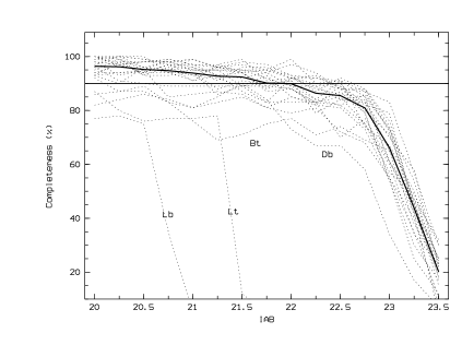
Figure 2: Variation of the completeness level as a function of I magnitude for 24 different regions of the image (each CCD was split horizontally into 2 equal sub-areas labelled t (top) and b (bottom)). The thick curve shows the completeness averaged over all CCDs but L. The thick horizontal line indicates the 90$\%$ completeness level.

We have carried out simulations to compute the completeness level. We added artificial objects (similar to real objects) to our image and measured the fraction of these objects recovered by the SExtractor package as a function of magnitude and location in the image. For this, we used a code created by J.M. Deltorn and already applied to the CFDF survey (e.g. McCracken et al. 2001) to compute the star detection completeness level. We modified this code in order to have a more realistic representation for galaxies, and used a gaussian profile with a FWHM of 3 times the mean seeing of our observation. The results are given in Fig. 2. This figure represents the percentage of completeness level as a function of I magnitude for 24 different regions of the total image (each CCD was split horizontally into 2 equal sub-areas). CCD L is significantly less complete than the other CCDs, because of many dead columns, and was removed in the following analyses. For the other CCDs, the mean completeness level is close to 90$\%$ up to ${\rm I_{AB}}$=22, which will be taken as the 90% completeness limit for our catalogue. We also obtained another estimation of our completeness level by comparing our observations with those of the CFDF survey (e.g. McCracken et al. 2001), which used the same instrument and filter, but with an exposure time of 5.5 hours and a seeing of 1 arcsec, and was complete up to I=25.6. Their completeness limit rescaled to our exposure time gives a completeness level at I=21.8, in agreement with our simulations. We will not attempt to correct our counts for incompleteness at magnitudes fainter than ${\rm I_{AB}}$=22, and we will hereafter limit our analysis to ${\rm I_{AB}}\leq$22.

In order to estimate the influence of “crowding” we computed the number of galaxies susceptible to be masked by bright galaxies. For 18$\leq{\rm I_{AB}}\leq$22 there are 9726 galaxies in an area of $1.007\times 10^{8}$ pixels² (entire field). As a conservative approach, we consider that galaxies brighter than ${\rm I_{AB}=18}$ and with surfaces larger than 600 pixels² can mask faint galaxies. The total surface covered by these galaxies is 24130 pixels², leading to a number of galaxies in the 18$\leq{\rm I_{AB}}\leq$22 magnitude interval that can be masked of the order of a few. Therefore, the influence of crowding on our study appears to be negligible.

3 Estimating the background contamination

Since the galaxy-star separation becomes difficult for magnitudes ${\rm I_{AB}}>20$, we decided to subtract the star and background galaxy contaminations statistically.

3.1 Star counts

In order to subtract the stellar contribution from our Galaxy, we produced a catalogue of stars using the Besançon model (Gazelle et al. 1995) in the I Kron-Cousins band in the direction of Abell 496. The relation between the magnitudes measured with the two filters is again: ${\rm I_{AB}}$=I${}_{\rm Besancon}+0.456$. The uncertainty on the star counts is smaller than 10% for ${\rm I_{AB}}\leq$22 (A. Robin, private communication), and the contribution of stars remains small in any case (less than one tenth of the total counts in our image, all objects considered), so star counts cannot influence our galaxy counts by more than a few percent in the magnitude interval 17$\leq{\rm I_{AB}}\leq 22$. An alternative way to perform this correction would have been to use the VIRMOS star counts, which have the advantage of having been obtained with the same CFH12K camera and filter, but they are not representative of the stellar counts in the direction of Abell 496, due to their lower Galactic latitude.

3.2 Field galaxy counts

Figure 3: Field galaxy counts from the VIRMOS survey (dashed line) and from Postman et al. (1998) (full line) a magnitude shift of +0.456, normalized to the total area of 1123 arcmin² covered by our catalogue. The galaxy counts derived from the outer regions of our Abell 496 field as explained in the text (Sect. 3.2.) are also shown.

An obvious way to correct for the background galaxy contribution would be to extract from our image a region as far as possible from the cluster center, subtract to it the star contribution and subtract the resulting galaxy counts to our data. We have extracted such an “outer zone” by putting together the data of the left half of CCD A and the right halves of CCDs F and G, and derived the galaxy counts in this zone. As can be seen in Fig. 3, these counts are higher than those issued from two independent field surveys (see below), once all are normalized to the same surface area (the total size of our image, i.e. 1123 arcmin²), suggesting that the Abell 496 “outer counts” thus produced still contain a significant fraction of cluster member galaxies, as confirmed by the positions of cluster galaxies in Fig. 1. So we would obviously overestimate the background if we took it in this “outer zone”. Note that our image covers a total region of 2.404$\times$1.584 Mpc², while the r₂₀₀ radius calculated as in Carlberg et al. (1997) with a velocity dispersion of 715 km/s (Durret et al. 2000) is 2.5 Mpc, confirming that the cluster contribution in the outer regions of our image is non negligible. Besides, the fact that the last point of the counts in the outer zone (${\rm I_{AB}}$=23.75) does not merge with any of the field survey background counts described below adds still another reason to reject this type of background subtraction.

We therefore decided to subtract the background contribution taken from the VIRMOS survey galaxy counts (McCracken et al. in preparation). However, the background galaxy contribution taken from this survey shows an excess of objects at magnitudes brighter than ${\rm I_{AB}}$=18.5, and cannot be directly subtracted to our counts either (see Fig. 3). The comparison of the galaxy counts by Postman et al. (1998) to the VIRMOS galaxy counts shows similar slopes for ${\rm I_{AB}}\geq$18.5 (see Fig. 3), with a magnitude shift due to the fact that the VIRMOS counts are in ${\rm I_{AB}}$ magnitudes while the Postman counts (which match well other counts such as those of Cabanac et al. 2000) are in Cousins I magnitudes. Shifting the Postman counts by 0.456 magnitude (see Sect. 2.1) gives a good agreement between both background counts for ${\rm I_{AB}}\geq$18.5. We will therefore subtract to our data the Postman galaxy counts shifted by 0.456 magnitude for 17$\leq{\rm I_{AB}}\leq$18.5 and the VIRMOS galaxy counts for 18.5$<{\rm I_{AB}}\leq$22. The star and background galaxy subtractions were performed in bins of 0.5 magnitude. The error bars that we indicate in the plots are simply computed as the square root of the number of galaxies in the corresponding magnitude bin.

4 Fitting method and results

4.1 Fitting method

Schechter function fits were performed using an IDL code based on the $curvefit$ function, which uses a gradient-expansion algorithm to compute a non-linear least squares fit to a given function; this routine gives the best fit parameters and respective errors of the Schechter function:

$$\Phi(M)dM=K\Phi^{*}10^{0.4(M^{*}-M)(\alpha+1)}\exp(-10^{0.4(M^{*}-M)})$$

where $\Phi^{*}$ is the normalisation, $M^{*}$ the characteristic apparent magnitude, $\alpha$ the slope of the faint end of the luminosity function and $M$ the apparent magnitude of a given galaxy in the I band.

4.2 Overall galaxy luminosity function

Figure 4: Galaxy counts in the direction of Abell 496 (dot-dashed line), background galaxy counts – see Sect. 3.2 (dashed line), and final galaxy luminosity function for Abell 496 after background subtraction (full line) with its error bars.

The resulting GLF for the entire field (after eliminating CCD L, the top half of CCD B: Bt and the bottom half of CCD D: Db) is shown in Fig. 4. A single Schechter function was fit in the same magnitude interval that we have been using (17$\leq{\rm I_{AB}}\leq$22, $-19.5\leq{\rm M_{I}}\leq-14.5$), giving a power law index slope $\alpha=-1.79\pm 0.01$. Results are given in Table 1 for all regions that we explore. For each case, we indicate the reduced $\chi^{2}$; all values are about 1 or lower, indicating that the fits are correct. Since $M^{*}$ is brighter than the lower limit of the magnitude interval considered here, it is not well constrained and we will therefore focus our discussion on the values of the slope $\alpha$ only. The correlation between $\alpha$ and $M^{*}$ is shown as confidence ellipses in Fig. 5 for various regions. The ellipses confirm that the error bars that we give on $\alpha$ in Table 1 are realistic. Note that the error bars in Table 1 are 1$\sigma$ error bars and correspond to the innermost ellipses in Fig. 5. We made tests on region CDIJ (see below), to see how an underestimate of the error bars could modify the slope of the GLF. For this, we multiplied the error bars by factors of 2 and 10 and found that $\alpha$ remains unchanged (even though our fitting procedure takes the error bars into account), while the uncertainty on $\alpha$ increases to $\pm 0.05$ and $\pm 0.1$ respectively, instead of the previous value of $\pm 0.03$. In order for our results to lose significance, we would have to multiply the error bars by 10, which seems an unrealistically large number (as seen for example from the scatter in the Metcalfe et al. Fig. 13). A factor of 2 seems much more probable, and in this case the difference in slopes between CDIJ and other regions remains significant.

Figure 5: Correlation between the two parameters M^∗ and $\alpha$ of the Schechter function for six regions: all the cluster, ABK, CDIJ (top row), EFGH, F and C (bottom row). The isocontours are 1, 2 and 3$\sigma$ respectively.

Table 1: Schechter law parameters for the various regions.

Region	Nb.	Area	$\alpha$	$\chi^{2}_{red}$
	gal.	(arcmin2)
All∗	4052	1031	$-1.79\pm 0.01$	7.26/7
ABK	1217	281	$-1.93\pm 0.02$	4.14/7
CDIJ	1542	378	$-1.75\pm 0.03$	1.50/7
EFGH	1652	372	$-1.98\pm 0.03$	1.80/7
CenL	426	94	$-1.82\pm 0.04$	1.80/7
CenM	292	53	$-1.79\pm 0.07$	0.48/7
CenS	129	24	$-1.60\pm 0.25$	1.50/7
A	409	93	$-2.05\pm 0.05$	3.60/7
B	402	94	$-1.73\pm 0.04$	3.18/7
C	312	95	$-1.73\pm 0.05$	3.60/7
D	353	94	$-1.87\pm 0.04$	3.36/7
E	364	94	$-1.68\pm 0.13$	1.98/7
F	460	92	$-2.03\pm 0.05$	2.34/7
G	297	92	$-1.87\pm 0.11$	2.76/7
H	534	94	$-2.03\pm 0.05$	4.08/7
I	374	94	$-1.60\pm 0.10$	0.66/7
J	505	94	$-1.78\pm 0.08$	2.46/7
K	407	94	$-1.94\pm 0.05$	4.08/7

^∗ All but L,Bt,Db

4.3 Galaxy luminosity function in three large regions

Figure 6: Galaxy luminosity function in various regions of Abell 496 (see text and Table 1).

We then divided the cluster into three regions of roughly equal surface, CDIJ surrounding the cluster center (CCDs C, D, I and J), ABK (CCDs A, B, K) towards the East and EFGH (CCDs E, F, G, H) towards the West. The GLFs in these three regions are shown in Fig. 6. The fit of the GLF by a Schechter function in region CDIJ is displayed in Fig. 7 (the fit was done in the interval 17$\leq{\rm I_{AB}}\leq$22 even though the figure shows the GLF in a larger range of magnitudes, for which we also extrapolated this best fit).

Figure 7: GLF in the central region (CDIJ) of Abell 496 with the best fit Schechter function superimposed.

The slope of the GLF is found to be flatter in region CDIJ, the Schechter law slopes being $\alpha=-1.75\pm 0.03$, $-1.93\pm 0.02$, and $-1.98\pm 0.03$, for regions CDIJ, ABK and EFGH respectively (see Table 1).

4.4 Mapping the parameters of the galaxy luminosity function

The GLFs in the 11 CCDs (L excluded) are shown in Fig. 6 and Table 1. Here also, the Schechter function slope may be steeper in the outer regions of the cluster, but better statistics are obviously required.

Finally, we selected three rectangular concentric regions of different sizes centered on the intersection of CCDs C, D, I and J (or, roughly the position of the cD cluster galaxy). CenL (Large), is of the size of a CCD and covers one quarter of CCDs C, D, I and J. CenM (Medium), covers 9/16 of the area of CenL. CenS (Small), covers 1/4 of CenL. The Schechter fits of the luminosity functions give slopes $\alpha=-1.82\pm 0.04,-1.79\pm 0.07$ and $-1.60\pm 0.25$ for CenL, CenM and CenS respectively, consistent with that in the CDIJ area within error bars. Region CenS may exhibit a flatter slope, but this needs confirmation since the uncertainty is very large.

5 Discussion and conclusions

We have derived the GLF in various regions of Abell 496. The slope of the Schechter function fit is always found to be steep (between $-1.60$ and $-2.05$). Since such a steep slope could be due to several artefacts, we will discuss the validity of our results. First, the background counts could have been underestimated. However, the good agreement of the various background counts (VIRMOS, Postman, Cabanac), and the fact that the subtraction is mainly that of the VIRMOS counts (in the interval 18.5$<{\rm I_{AB}}\leq$22), made with the same instrument, filter and magnitude system as ours, tends to suggest that this is not the case. Second, the number of faint galaxies may have been overestimated; for example, we may have confused globular clusters with galaxies at faint magnitudes, as explained in detail by Andreon & Cuillandre (2002). However, we limit our sample to ${\rm I_{AB}}$=22, where such effects should not be too strong. Third, our ${\rm I_{AB}}$ magnitudes may be too bright by 0.25 magnitude, as suggested by the difference with the Moretti et al. data (see Sect. 2.1). We tried to fit the GLF in several regions after shifting the ${\rm I_{AB}}$ magnitudes by 0.25 (before subtracting the background) and find slopes $\alpha=-1.68\pm 0.05,-1.85\pm 0.03$ and $-1.94\pm 0.04$ for regions CDIJ, ABK and EFGH respectively, instead of the previous values of $-1.75,-1.93$ and $-1.98$. Therefore, although the values change a little, the slope remains flatter in CDIJ.

We then used our ${\rm I_{AB}}$ catalogue limited to the region in common with Molinari et al. (1998) and made a Schechter fit as described above. The Molinari et al. zone partially covers our CCDs J,I,C,D,E and F, with a main concentration towards CCD E. A Schechter fit in the same magnitude interval gives a slope $\alpha=-1.71\pm 0.06$, close to the value of $-1.68\pm 0.13$ found in CCD E. A shift of ${\rm I_{AB}}$ by 0.25 magnitude as above gives $\alpha=-1.68\pm 0.09$, in perfect agreement with Molinari. Fits in broader magnitude intervals give: $\alpha=-1.66\pm 0.05,-1.64\pm 0.04$ and $-1.57\pm 0.03$ for the magnitude intervals 17$\leq{\rm I_{AB}}\leq$22.5, 17$\leq{\rm I_{AB}}\leq$23, and 17$\leq{\rm I_{AB}}\leq$23.5 respectively. Molinari et al. give a slope $\alpha=-1.49\pm 0.04$ in the i band, but mention that a magnitude correction allows them to reach a slope as steep as $\alpha=-2.0$. We therefore believe that our results are consistent with theirs. Note that such a slope is not much steeper than found e.g. in Coma (Lobo et al. 1997) or in Abell 665 (De Propris et al. 1995). This could indicate an excess of faint red galaxies, but to ascertain this hypothesis it would be necessary to derive the GLF in Abell 496 in other filters from samples of comparable quality (covered area and depth). As still another test on the robustness of our results, we reanalyzed the GLF in the CDIJ region. For this, we reduced the number counts by 10, 20, 30 40 and 50% for ${\rm I_{AB}}>$20 (below ${\rm I_{AB}}$=20 the counts remained unchanged) and made fits of these new GLFs. Results are given in Table 2. They show that the slope changes strongly only if the counts are reduced by at least 30%, an unrealistic number. Besides, in order to account for the difference in slope of 0.2 that we observe for example between regions CDIJ and EFGH, we would need to make an unrealistically large error of 50% on the counts. We are therefore confident that both the absolute values of $\alpha$ and their variations from one zone to another are robust.

Our second result is that the slope of the Schechter function fit tends to be steeper in the outer regions of the cluster, as already observed in other clusters (see references in Sect. 1). Such a variation of $\alpha$ can be interpreted as due to the fact that faint galaxies are accreted by larger ones preferentially in the inner parts of clusters, where the galaxy density is higher, therefore inducing a lack of faint galaxies and a flattening of the GLF in the inner regions. Moreover, galaxies are likely to have suffered repeated tidal interactions on their way towards the cluster center, consequently being dimmed or even disrupted in a scenario of galaxy harassment (Moore et al. 1996).

The next step is obviously to confirm these results through deep multiband imaging and/or spectroscopy that would make the background subtraction more secure and would allow us to compare the GLFs in various filters.

Table 2: Schechter law slope when the counts are reduced.

Reduction of	New values
counts	of $\alpha$
0%	$-1.75\pm 0.03$
10%	$-1.72\pm 0.04$
20%	$-1.68\pm 0.03$
30%	$-1.61\pm 0.03$
40%	$-1.59\pm 0.02$
50%	$-1.48\pm 0.04$

References

- Adami C. et al. (1998) Adami C., Nichol R., Mazure A. et al. 1998, A&A 334, 765
- Adami C. et al. (2000) Adami C., Ulmer M., Durret F. et al. 2000, A&A 353, 930
- Andreon (2002) Andreon S. 2002, A&A 382, 821
- Andreon & Cuillandre (2002) Andreon S., & Cuillandre J.C. 2002, ApJ 569, 144
- Beijersbergen et al. (2002) Beijersbergen M., Hoekstra H., van Dokkum P.G., & van der Hulst T. 2002, MNRAS 329, 385
- Bertin & Arnouts (1996) Bertin E., & Arnouts S. 1996, A&AS 117, 393
- Biviano et al. (1995) Biviano A., Durret F., Gerbal D. et al. 1995, A&A 297, 610
- Cabanac, de Lapparent & Hickson (2000) Cabanac R.A., de Lapparent V., & Hickson P. 2000, A&A 364, 349
- Carlberg et al. (1997) Carlberg R.G., Yee H.K.C., Ellingson E. et al. 1997, ApJ 485, L13
- De Propris (1995) De Propris R., Pritchet C.J., Harris W.E., & McClure R.D. 1995, ApJ 450, 534
- Driver et al. (1998) Driver S.P., Couch W.J., & Phillipps S. 1998, MNRAS 301, 369
- Durret et al. (1999a) Durret F., Gerbal D., Lobo C., & Pichon C. 1999a, A&A 343,760
- Durret et al. (1999b) Durret F., Felenbok P., Lobo C., & Slezak E. 1999b, A&AS 139, 525
- Durret et al. (2000) Durret F., Adami C., Gerbal D., & Pislar V. 2000, A&A 356, 815
- Fukugita et al. (1995) Fukugita M., Shimasaku K. & Ichikawa T., 1995, PASP 107, 945
- Gazelle et al. (1995) Gazelle F., Robin A., & Goidet-Devel B. 1995, Vistas in Astronomy 39, 105
- Godwin & Peach (1977) Godwin J.G., & Peach J.V. 1977, MNRAS 181, 323
- Kajisawa et al. (2000) Kajisawa M., Yamada T., Tanaka I. et al. 2000, PASJ 52, 53
- Landolt (1992) Landolt A.U., 1992, AJ 104, 340
- Lobo et al. (1997) Lobo C., Biviano A., Durret F. et al. 1997, A&A 317, 385
- McCracken et al. (2001) McCracken H.J., LeFèvre O., Brodwin M. et al. 2001, A&A, 376, 756
- Molinari et al. (1998) Molinari E., Chincarini G., Moretti A., & De Grandi S. 1998, A&A 338, 874
- Moore et al. (1996) Moore B., Katz N., Lake G., Dressler A., & Oemler A. 1996, Nature 379, 613
- Moretti et al. (1999) Moretti A., Molinari E., Chincarini G., & De Grandi S. 1999, A&AS 140, 155
- Phillipps et al. (1998) Phillipps S., Driver S.P., Couch W.J., & Smith R.M. 1998, ApJ 498, L119
- Slezak et al. (1999) Slezak E., Durret F., Guibert J., & Lobo C. 1999, A&AS 139, 559