Line-of-sight Effects on Observability of Kink and Sausage Modes in Coronal Structures with Imaging Telescopes

Kink modes of solar coronal structures, perturbing the loop in the direction along the line-of-sight (LOS), can be observed as emission intensity disturbances propagating along the loop provided the angle between the LOS and the structure is not ninety degrees. The effect is based upon the change of the column depth of the loop (along the LOS) by the wave. The observed amplitude of the emission intensity variations can be larger than the actual amplitude of the wave by a factor of two and there is an optimal angle maximizing the observed amplitude. For other angles this effect can also attenuate the observed wave amplitude. The observed amplitude depends upon the ratio of the wave length of kink perturbations to the width of the structure and on the angle between the LOS and the axis of the structure. Sausage modes are always affected negatively from the observational point of view, as the observed amplitude is always less than the actual one. This effect should be taken into account in the interpretation of wave phenomena observed in the corona with space-borne and ground-based imaging telescopes.

1 Introduction

In last few years, significant progress in the observational study of MHD wave activity of the solar corona has been achieved with SOHO/EIT and TRACE EUV imaging telescopes. Flare-generated decaying oscillations of coronal loops have been observed and interpreted as kink fast magnetoacoustic modes of the loops (Aschwanden et al. 1999; Nakariakov et al. 1999; Schrijver & Brown 2000; Aschwanden et al. 2002). Fast magnetoacoustic waves are possibly responsible for events such as coronal Moreton (or EIT) waves (Thompson et al. 1998, Ofman & Thompson 2002). Slow magnetoacoustic waves have been discovered in polar plumes (Ofman et al. 1997; DeForest & Gurman 1998; Ofman, Nakariakov & DeForest 1999) and in long loops (Berghmans & Clette 1999; De Moortel, Ireland, Walsh 2000; Nakariakov et al. 2000; De Moortel 2002 ). These observational breakthroughs give rise to the use of MHD coronal seismology (Nakariakov et al. 1999; Robbrecht et al. 2001; Nakariakov & Ofman 2001) and were interpreted to support the idea of wave-based theories of coronal heating (e.g., Tsiklauri & Nakariakov 2001), and the solar wind acceleration (e.g., Ofman, Nakariakov & Seghal 2000).

Slow and fast magnetoacoustic waves are compressive and cause perturbations of plasma density. As an emission depends upon the density, the waves can be detected as the emission variations by imaging telescopes. An important characteristic of the phenomenon is the angle between the direction of the wave propagation and the line of sight (LOS). Imaging telescopes allow us to observe magnetoacoustic waves propagating at sufficiently large angles to the LOS. In particular, this fact motivated the interpretation of the propagating EUV emission disturbances as slow magnetoacoustic waves (see the references above). In addition, Alfvén waves, which are linearly incompressible, as well as almost incompressible kink modes of coronal magnetic structures (e.g., Roberts 2000 and references therein), can also be detected with an imaging telescope with sufficient spatial and temporal resolution, if perturbations of the magnetic field have a component perpendicular to the LOS. Indeed, as the magnetic field is frozen into the coronal plasma, the perpendicular displacement of the field can be highlighted by variation of emission intensity.

In this paper we discuss an alternative method for the observational detection of kink modes of coronal magnetic structures oscillating in the plane containing the LOS. It is shown that this would lead to modulation of the intensity of the emission along the axis of the structure, produced by the change of the LOS column depth of the loop. We also demonstrate that this phenomenon is important for sausage modes.

2 Kink modes of cylindric magnetic structures

Kink modes of coronal loops, observed in particular, with the TRACE EUV imaging telescope (see the references above), are periodic transverse displacements of the magnetic flux tube forming the loop. They should be distinguished from sausage modes which do not perturb the tube axis. Modeling the loop tube as a straight magnetic cylinder uniform along the axis, Edwin & Roberts (1983) found that the kink modes can be either surface or body, depending upon the structure of the mode inside the tube. Also, the modes can be slow or fast, corresponding to fast and slow magnetoacoustic waves modified by the structuring of the medium. In particular, in the low-$\beta$ plasma of the solar corona, coronal loops can support fast and slow kink body modes.

In the case of a kink mode the loop tube oscillates almost as whole and the cross-section of the loop is practically not perturbed by the oscillation. Also, the density perturbation inside the loop is insignificant in this mode. Indeed, for fast magnetoacoustic waves in a low-$\beta$ coronal plasma, the field-aligned flows $V_{z}$ are much smaller than the transverse motions $V_{x}$. Consequently, from the continuity equation, one gets that the density perturbations $\tilde{\rho}$ are connected with the transverse perturbations by the expression

$$\frac{\tilde{\rho}}{\rho_{0}}\approx\sqrt{1-C_{A0}^{2}k^{2}/\omega^{2}}\ \frac{V_{x}}{C_{A0}},$$ (1)

where $\rho_{0}$ and $C_{A0}$ are the density and the Alfvén speed inside the loop tube, respectively, and other notations are standard. As the frequency $\omega$ of the fast kink mode of a coronal loop tends to the value $C_{A0}k$ with the increase of the wave number $k$ (Edwin & Roberts 1983, Fig. 4), the coefficient on the right hand side of Eq. (1) tends to zero in the same limit. Consequently, the fast kink mode is almost incompressible. We would like to stress that the characteristic spatial scale of the mode inside the loop tube is quite different from the loop tube diameter. In the limit $\omega/k\to C_{A0}$, the characteristic transverse scale inside the tube tends to infinity, i.e., inside the tube diameter the density is not perturbed. Outside the tube, the scale is different and it determines the mode localization length, which is about $\sqrt{\omega^{2}/C^{2}_{Ae}-k^{2}}$, where $C_{Ae}$ is the Alfvén speed in the external medium. Consequently, outside the loop tube, the kink mode can be quite compressible.

The fast kink mode is often confused with the true incompressible Alfvén mode. However, the Alfvén mode modified by structuring is the torsional mode which, in the linear limit and cylindrical geometry, does not perturb the tube boundary.

Consider a kink mode which symmetrically perturbs the boundary of the loop tube. The wavelength is assumed to be much shorter than the loop length, so the loop can be considered as a straight cylinder. The plane of the transverse oscillations produced by the kink mode forms an angle $\alpha$ with the line-of-sight (LOS). In the following, we assume that the angle $\alpha$ is zero, i.e. LOS is co-planar with the plane of oscillation. The tube axis has an angle $\theta$ with LOS (see Figure 1). We neglect the perturbations of density by the mode, assuming that the density is equal to the unperturbed density $\rho_{0}$. The tube diameter is $w$. We also assume that the diameter of the tube does not change in time and space. The intensity of the emission $I$ produced by the loop is proportional to the LOS column depth of the loop tube $l$ and to the density of the plasma squared,

$$I\propto\rho_{0}^{2}l.$$ (2)

In the absence of the perturbations, the intensity $I$ along a straight segment of the loop is constant, $I\propto\rho_{0}^{2}w/\sin\,\theta$.

When the loop experiences kink perturbations, the column depth $l(d,t)$ of the loop tube depends upon the coordinate $d$ along the loop (taking into account the effect of projection, see Fig. 1) and changes with time $t$. As, in the optically thin medium, the intensity of the emission is proportional to thickness of the volume of plasma emitting the radiation, the variation of the LOS column depth causes the variation of the intensity. Thus, the emission intensity variations can be produced even by entirely incompressible kink waves, and consequently, by the almost incompressible kink modes of coronal loops.

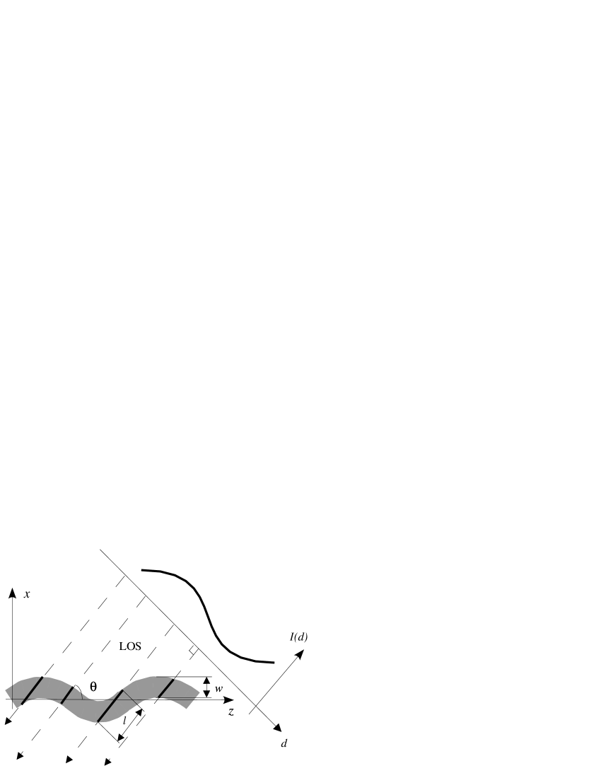
Figure 1: A snapshot of perturbation of a segment of a coronal loop by a harmonic kink wave and produced variations of the emission intensity along the loop image. The variations produce the change of the LOS column depth of the loop if the angle $\theta$ between the loop axis and the line-of-sight differs from ninety degrees. The variations of the column depth of the loop modulate the emission intensity $I(d)$ on the loop image.

Note that the density perturbations produced by the wave outside the loop are ignored in Eq. (2), as the external plasma is observed to be much more rarefied.

3 Parametric studies

3.1 Kink modes

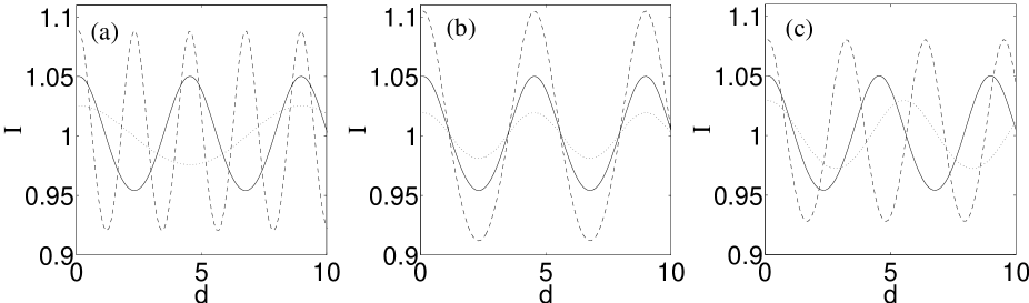
Figure 2: The effect of changing wavelength (a), wave amplitude (b) and viewing angle (c) respectively on the observed emission intensity variations along a straight segment of a coronal loop in the presence of a harmonic kink wave. The intensity $I$ is normalized to the unperturbed intensity in the absence of the wave. The distance $d$ is normalized to the loop diameter. On the left panel, the dotted curve corresponds to the wavelength $\lambda=4\pi$, the solid to $\lambda=2\pi$ and the dashed to $\lambda=\pi$, measured in loop diameters. For all curves, the normalized wave amplitude is $a=0.05$ and the angle between the loop axis and the LOS is $\theta=\pi/4$. On the middle panel, the dotted curve corresponds to $a=0.02$, the solid to $a=0.05$ and the dashed to $a=0.1$, for $\lambda=2\pi$ and $\theta=\pi/4$. On the right panel, the dotted curve corresponds to $\theta=\pi/3$, the solid to $\theta=\pi/4$ and the dashed to $\theta=\pi/6$, for $a=0.05$ and $\lambda=2\pi$.

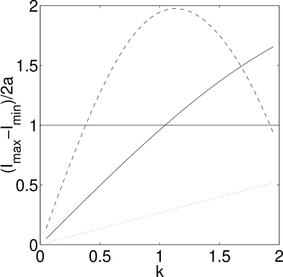
Figure 3: Dependence of the observed amplitude of emission intensity variations along a straight segment of a coronal loop in the presence of a harmonic kink wave upon the wave number $k$, normalized to the loop diameter and the wave amplitude, which is 0.05 for all three curves. The dotted curve corresponds to the angle between the loop axis and the LOS $\theta=5\pi/12$ $(75\degr)$, the solid to $\theta=\pi/4$ $(45\degr)$ and the dashed to $\theta=\pi/9$ $(20\degr)$. The solid horizontal straight line indicates the actual normalized wave amplitude. Points above this line indicate amplification while points below indicate attenuation.

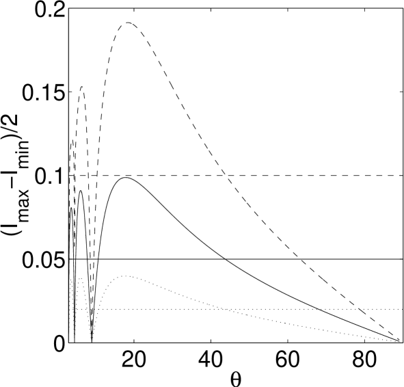
Figure 4: Dependence of the observed amplitude of emission intensity variations along a straight segment of a coronal loop in the presence of a harmonic kink wave upon the angle between the loop axis and the LOS $\theta$. The dotted curve corresponds to the wave amplitude $a=0.02$, the solid to $a=0.05$ and the dashed to $a=0.1$, for the normalized wavelength $\lambda=2\pi$. Similarly the straight horizontal lines represent the actual amplitude of their respective waves. Points above these lines indicate amplification while points below indicate attenuation.

Consider a snapshot of a harmonic kink perturbation of a straight tube modeling a segment of a coronal loop. At a given time, boundaries of the tube are given by the equations

$$x=a\sin\left(kz\right)\pm\frac{w}{2},$$ (3)

where $a$ is the perturbation amplitude and $k$ is the wave number ($k=2\pi/\lambda$ where $\lambda$ is the wavelength), and the plus and minus signs correspond to the upper and lower boundaries, respectively. The geometry of the problem is shown in Fig. 1. Observing the tube at an angle $\theta$, we see that the LOS column depth of the tube is modulated by the kink perturbation. The family of parallel LOS is given by the equation

$$x=z\tan\theta-d/\cos\theta,$$ (4)

where the parameter $d$ represents the coordinate across the LOS and, consequently, along the image (see Fig. 1).

Solving the set of equations (3) and (4), we find the intersections of the LOS with the tube boundaries. We then have two points, one where the LOS enters the tube and one where it exits. Using these points we can determine the column depth of the tube along a given LOS as a function of the coordinate $d$ along the image. Note that the line of sight may pass into and out of the flux tube more than once for certain amplitudes, LOS angles and wave numbers. We must therefore take into account all solutions of the set (3)-(4) and whether the line of sight is inside or outside of the tube. The LOS passing through the tube more than once only occurs if the gradient of the normal to the LOS is greater than the minimum gradient of equations (3), i.e.

$$ak>\frac{1}{\tan\theta}.$$ (5)

Thus, we determine the LOS column depth of the tube as a function of the position on the image, which, if the density of plasma inside the tube and the width of the tube across the LOS remain constant, is proportional to the intensity of the emission coming from the tube. The intensity is normalized to the intensity given by a tube at the same angle to the LOS but with zero amplitude waves, $a=0$. This measures the effect the presence of waves have on intensity.

Figures 2–4 demonstrate how the effect discussed depends upon the parameters of the problem. Fig. 2 shows the distribution of the emission intensity along the tube on an image for different wavelengths and amplitudes of the kink mode and the observation angles $\theta$. Obviously, the observed variation of the emission intensity is proportional to the amplitude of the wave and it decreases with the increase of the wavelength. Indeed, in the limiting case when the wavelength tends to infinity, the LOS column depth of the tube does not change and the effect vanishes. The observed amplitude is calculated as the difference between the maximum and the minimum values of the observed intensity, divided by two. The dependence of the observed amplitude of the intensity perturbations upon the wave number of the kink wave is shown in Fig. 3. We gather from this graph that: For the $75\degr$ dotted line there is a decrease in the attenuation with increasing $k$ for $0<k<2$; for the $45\degr$ solid line, for $0<k\lesssim 1$, there is a decrease in the attenuation with increasing $k$, while for $1\lesssim k<2$ there is an increase in the amplification; for the $20\degr$ dashed line, for the range of $k$’s conisdered, there is an optimal wave number corresponding to the maximum amplification. To graphical accuracy the $75\degr$ and $45\degr$ curves with amplitudes $a=0.02$ and $a=0.1$ are identical to the $a=0.05$ curves and the $a=0.02$ and $a=0.1$, $20\degr$ curves (not plotted) lie very close to the $a=0.05$ dashed curve. Therefore non-linear amplitude effects within the parameter regimes considered are small to observational accuracy and not considered further here.

According to the right panel of Fig. 2 and Fig. 4, the dependence of observed amplitude of the intensity variations upon the angle $\theta$ has a pronounced maximum, corresponding to an optimal angle of the wave detection. Indeed, the effect of the modulation of the observed intensity by a kink wave vanishes when the angle tends to $\pi/2$, while the whole approach fails when $\theta\to 0$ (the leftmost data points in Fig. 4 correspond to $\theta=3^{\circ}$). Fig. 4 clearly demonstrates, however, that there is an optimal angle which yields the maximum observed amplitude. Thus, this phenomenon would make it possible to observe kink modes in a certain segment of a coronal loop (in the realistic curved geometry), where the angle $\theta$ is optimal. This optimal angle varies with $k$ and weakly with $a$, figure 5. It corresponds closely to a LOS passing through a maximum of the upper curve and a neighboring minimum of the lower curve (see equations (3)). Similarly, there can be other optimal angles, if the LOS passes through a maximum of the upper curve and another minima of the lower curve. This estimation for the optimal angles $\theta_{max}$ gives

$$\theta_{max}=\arctan\left[\frac{k\left(w+2a\right)}{2\pi\left(n-\frac{1}{2}\right)}\right],$$ (6)

where $n=1,2,3...$ is the peak number with decreasing $\theta$. The highest three rightmost peaks (for the same $\theta$, but different amplitudes) in figure 4 correspond to $n=1$. Peaks corresponding to the higher values of $n=2$ and $3$ are progressively smaller than the peaks at $n=1$. It is possible that the optimal angles smaller than this one corresponding to $n=1$ are not relevant to coronal applications, as for sufficiently small angles the curvature of the loop plays an important role. The loop may only be modeled by a straight cylinder if the approximately straight loop section is sufficiently long.

There are also angles corresponding to zero intensity variation, the first is at $\theta=90\degr$ (see Fig. 4). Here a LOS passes through the maxima of both curves and the angles are given by

$$\theta_{min}=\arctan\left[\frac{kw}{2\pi n}\right].$$ (7)

When the angle is about these values the observed amplitude is attenuated and at these zero points kink waves may not be detected at all. Note that these points do not depend on amplitude. In figure 4 the straight horizontal lines at the respective wave amplitudes divide the graph into two regions; above, where the observed signal is amplified, and below, where it is attenuated. If these curves are normalized to the amplitude, $a$, then to graphical accuracy they collapse on top of each other everywhere except for the vicinity of the peaks where they are still close.

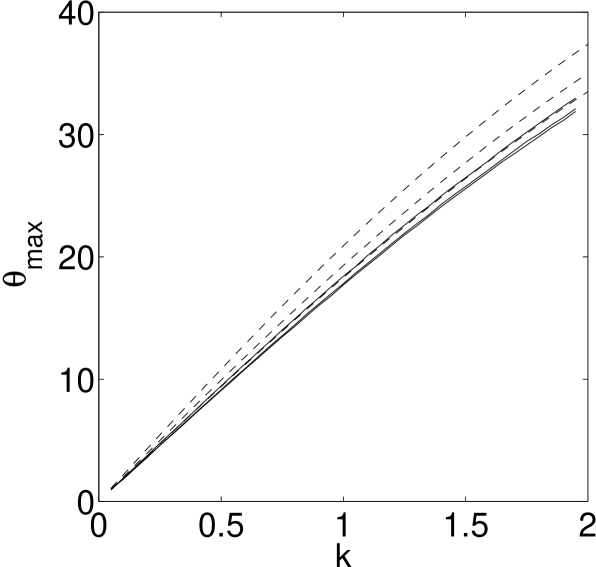
Figure 5: Dependence of the optimal observation angle along a straight segment of a coronal loop in the presence of a harmonic kink wave upon the wave number $k$. The solid curves corresponds to the actual optimal angles and the dashed correspond to equation (6) for the amplitude $a=0.1$, top, $a=0.05$, middle and $a=0.02$, bottom. Note that the deviation between theory (Eq.(6)) and numerical calculation is tolerably small, however, it grows with the increase of $a$ and $k$.

3.2 Sausage modes

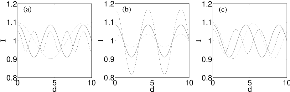
Figure 6: The effect of changing wavelength (a), wave amplitude (b) and viewing angle (c) respectively on the observed emission intensity variations along a straight segment of a coronal loop in the presence of a harmonic sausage wave. The parameters $\lambda$, $\theta$ and $a$ have identical values to those given in figure 2.

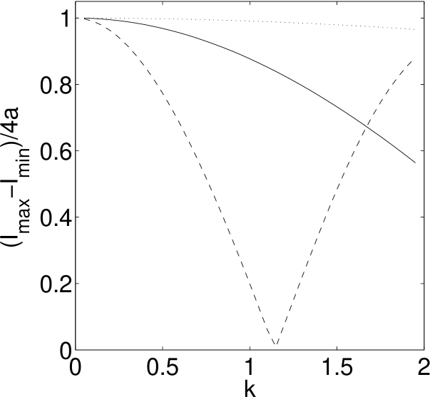
Figure 7: Dependence of the observed amplitude of emission intensity variations, normalized to twice the wave amplitude, along a straight segment of a coronal loop in the presence of a harmonic sausage wave upon the wave number $k$, normalized to the loop diameter. $a=0.05$ for all three curves. Curves of amplitudes $a=0.1$ and $a=0.02$ are almost identical to graphical accuracy. The dotted curve corresponds to twice the angle between the loop axis and the LOS $\theta=5\pi/12$ $(75\degr)$, the solid to $\theta=\pi/4$ $(45\degr)$ and the dashed to $\theta=\pi/9$ $(20\degr)$. Twice the normalized wave amplitude is at $(I_{max}-I_{min})/4a=1$. All points fall below this line, indicating attenuation of the expected measurements. The minimum of the $20\degr$ curve is of a similar nature to the minimum found in figures 4 and 8.

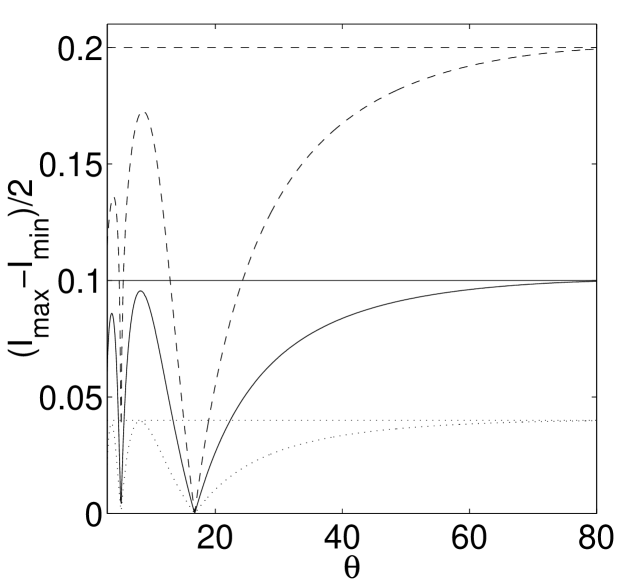
Figure 8: Dependence of the observed amplitude of emission intensity variations along a straight segment of a coronal loop in the presence of a harmonic sausage wave upon the angle between the loop axis and the LOS $\theta$. The dotted curve corresponds to the wave amplitude $a=0.02$, the solid to $a=0.05$ and the dashed to $a=0.1$, for the normalized wavelength $\lambda=2\pi$. The horizontal straight lines are added for comparison with figure 4 and correspond to the amplitude of the respective waves. Note that the amplitude at $90\degr$ gives the largest amplitude and therefore we only see attenuation below this.

Similarly, the effect discussed above should be important for sausage modes too. Indeed, as the sausage modes are the propagating perturbations of the loop tube cross-section, the LOS column depth of the loop is modulated by these waves too. To complete the picture, we now perform a study of the LOS effect on observability of sausage waves.

The boundaries of a straight tube exhibiting sausage oscillations can be given by the equations

$$x=a\sin\left(kz+\frac{\pi}{2}\right)+\frac{w}{2}$$ (8)

corresponding to the upper boundary and

$$x=a\sin\left(kz+\frac{3\pi}{2}\right)-\frac{w}{2}$$ (9)

corresponding to the lower boundary. The family of parallel LOS is given by equation (4). We solve these equations in the same way as for the kink oscillations. Figure 6 shows the distribution of emission intensity along the tube for the same parameters as those given in figure 2. The wavelength, $k$, and angle, $\theta$, at high angles have the opposite effect of kink oscillations on the amplitude intensity, figures 7 and 8. The best observation angle is $\theta=90\degr$ as expected. Note that the analysis here is two dimensional and the observed intensity amplitude would be increased for a three dimensional tube if the telescope pixel size is of the order of the tube width. However only the intensity scale of figures 6 to 8 would change and not the form. The optimum angle for the detection of sausage modes is still $90\degr$. The LOS only passes into and out of the tube once for the angles considered.

4 Conclusions

The phenomenon of the modulation of the emission intensity by kink modes polarized in the plane formed by the loop axis and the LOS provides a possibility for the observational detection of the kink modes in coronal structures. According to the discussion above, the LOS effect at an optimal angle, $\theta_{max}$, can amplify the kink perturbations by a factor of 2 (cf. Fig. 4). For example, if the boundary perturbation is produced by a kink mode of a relatively modest amplitude of about 5%, which corresponds to the typical coronal wave amplitudes detected by SOHO/EIT (DeForest & Gurman 1998) and by TRACE (e.g. De Moortel et al. 2002 and references therein), the observed perturbation of the intensity produced by the kink wave can reach 10%, which would make the wave easily observable. In contrast, the optimal observation angle for the sausage modes is simply $90\degr$ (cf. Fig. 8). Consulting figures 3 and 4 we can see parameter regimes for both amplification and attenuation of the kink mode observations. Figures 7 and 8 demonstrate that relative to $90\degr$ observations there is only attenuation of sausage modes. Additional observability constraints are connected with the wave period and length. In the case of EUV imaging coronal telescopes, such as EIT and TRACE, the observability of the waves is limited by the telescope time resolution. For example, taking the kink speed inside a loop to be 1000 km/s, which corresponds to the estimations in Nakariakov et al. 1999, Nakariakov & Ofman 2001, the time resolution of about 30 s does not allow us to observe wavelengths shorter than 30 Mm.

In the case of ground-based observations, when the loop is observed in the green line bandpass, the observability is limited by the spatial resolution of the telescope, which is usually over a few arcsec, as the time resolution of such observations is usually less then 1 sec (e.g, the cadence time of SECIS is 2.25$\times 10^{-2}$ s and the pixel size is 4.07 arcsec, Williams et al. 2001). In particular, this effect can be responsible for propagating 6 second disturbances of the Fe xiv green line, discovered by the stroboscopic method in a solar eclipse data and interpreted as fast magnetoacoustic waves (Williams et al. 2002, see also Williams et al. 2001). Indeed, estimating the wavelength of the perturbations at about 18 Mm (for the wave period of about 6 s and the propagation speed of about 2 Mm/s), we conclude that the waves are detectable with the time and spatial resolution of the telescope. For loop widths of about 3-6 Mm, the normalized wavelength is about 3-6, which gives the wavenumber $k$ of about 1-2. According to Fig. 3, the LOS effect discussed in this paper could amplify the observed amplitude of the wave, optimizing the observability of the modes. According to figure 5, for the parameters discussed, the optimal angle would be about $20\degr-40\degr$. This makes the phenomenon discussed here relevant to the interpretation of Williams et al. (2002)’s results. However, the confident interpretation of the propagating disturbances in terms of the kink waves requires detailed comparison of the observed results and theoretical predictions. Also, interpretation of these observations in terms of propagating kink modes should be tested against another possible interpretation of the waves as sausage modes. The study of the possible relevance of the LOS effect to the interpretation of short wavelength propagating waves observed in the corona by Williams et al. (2002) is now in progress and will be presented elsewhere.

Also, this phenomenon should be taken into account in the analysis of other examples of coronal wave activity, in particular the slow waves in loops and polar plumes, discussed in Introduction. However, direct application of the results presented in this paper to the coronal slow magnetoacoustic waves is not possible as the slow waves are essentially compressible, and the density variation should be taken into account in Eq. (2). This phenomenon should also be taken into account in interpretation of intensity oscillations observed in prominence fine structures (e.g. Joarder, Nakariakov & Roberts 1997; Diaz et al. 2001). This suggests another possible development of this study.

- (1) Aschwanden M.J., De Pontieu B., Schrijver C.J., Title A.M., 2002, Solar Phys. 206, 99
- (2) Aschwanden M.J., Fletcher L., Schrijver C.J. and Alexander D., 1999, ApJ 520, 880
- (3) Berghmans D., Clette F., 1999, Solar Phys. 186, 207
- (4) DeForest C.E., Gurman J. B., 1998, ApJ 501, L217.
- (5) De Moortel I., Ireland J., Walsh R.W., 2000, A&A 355, L23
- (6) De Moortel I., Hood A.W., Ireland J., Walsh R.W., 2002, Solar Phys. 209, 89
- (7) Díaz A.J., Oliver R, Erdélyi R., Ballester J.L., 2001, A&A 379, 1083
- (8) Edwin P.M., Roberts B., 1983, Solar Phys. 88, 179.
- (9) Joarder P.S., Nakariakov V.M., Roberts B., 1997, Solar Phys. 173, 81
- (10) Nakariakov V.M., Ofman L., 2001 A&A 372, L53
- (11) Nakariakov V.M., Ofman L., DeLuca E.E., Roberts B., Davila J.M., 1999, Sci. 285, 862
- (12) Nakariakov V.M., Verwichte E., Berghmans D., Robbrecht E., 2000, A&A 362, 1151
- (13) Ofman L., Nakariakov V.M., Deforest C.E., 1999, ApJ 514, 441
- (14) Ofman L., Nakariakov V.M., Sehgal N., 2000, ApJ 533, 1071
- (15) Ofman L., Romoli M., Poletto G., Noci G., Kohl J.L., 1997, ApJ 491, L111
- (16) Ofman L., Thompson B.J., 2002, ApJ 574, 440
- (17) Robbrecht E., Verwichte E., Berghmans D., Hochedez J.F., Poedts S., Nakariakov V.M., 2001, A&A 370, 591
- (18) Roberts B., 2000, Solar Phys. 193, 139
- (19) Schrijver C.J., Brown D.S., 2000, ApJ 537, L69
- (20) Thompson B.J., Plunkett S.P., Gurman J.B., Newmark J.S., St Cyr O.C., Michels D.J., 1998, Geophys. Res. Let. 25, 2465
- (21) Tsiklauri D., Nakariakov V.M., 2001, A&A 379, 1106
- (22) Williams D.R., et al., 2001, MNRAS 326, 428
- (23) Williams D.R., et al., 2002, MNRAS (in press)