Complex dynamics in a simple model of pulsations for Super-Asymptotic Giant Branch Stars

Abstract

When intermediate mass stars reach their last stages of evolution they show pronounced oscillations. This phenomenon happens when these stars reach the so-called Asymptotic Giant Branch (AGB), which is a region of the Hertzsprung-Russell diagram located at about the same region of effective temperatures but at larger luminosities than those of regular giant stars. The period of these oscillations depends on the mass of the star. There is growing evidence that these oscillations are highly correlated with mass loss and that, as the mass loss increases, the pulsations become more chaotic. In this paper we study a simple oscillator which accounts for the observed properties of this kind of stars. This oscillator was first proposed and studied in [1] and we extend their study to the region of more massive and luminous stars — the region of Super-AGB stars. The oscillator consists of a periodic nonlinear perturbation of a linear Hamiltonian system. The formalism of dynamical systems theory has been used to explore the associated Poincaré map for the range of parameters typical of those stars. We have studied and characterized the dynamical behaviour of the oscillator as the parameters of the model are varied, leading us to explore a sequence of local and global bifurcations. Among these, a tripling bifurcation is remarkable, which allows us to show that the Poincaré map is a nontwist area preserving map. Meandering curves, hierarchical-islands traps and sticky orbits also show up. We discuss the implications of the stickiness phenomenon in the evolution and stability of the Super-AGB stars.

]

I Introduction

The study of pulsating stars has attracted much attention from astronomers. Pulsational instabilities are found in many phases of stellar evolution, and also for a wide range of stellar masses (see [2] for an excellent review). Moreover, pulsational instabilities provide a unique opportunity to learn about the physics of stars and to derive useful constraints on the stellar physical mechanisms that would not be accessible otherwise. Within the theory of stellar pulsations, there are three basic characteristics of the motions that the associated model may include or not, namely the oscillations can be linear or nonlinear, adiabatic or not, and radial or nonradial [3]. Actual pulsations of real stars must certainly involve some degree of nonlinearity [4, 5, 6]. In fact, the irregular behaviour observed in many variable stars is, definitely, the result of those nonlinear effects [7]. Moreover, the fact that the observed pulsation amplitudes of variable stars of a given type do not show huge variations from star to star suggests the existence of a (nonlinear) limit-cycle type of behaviour [8]. However the full set of nonlinear equations is so complicated that there are no realistic stellar models for which analytic solutions exist and thus the investigations of nonlinear pulsations rely on numerical analysis. Accordingly, most recent theoretical studies of stellar pulsations proceed either through pure numerical hydrodynamical codes [9, 10, 11, 12, 13] or, conversely, they adopt a set of simplifying assumptions in order to be able to deal with a extraordinarily complex problem. Most of these simple models of stellar pulsation are based on a one-zone type of model which may be visualized as a single, relatively thin, spherical mass shell on top of a rigid core. These models have helped considerably in clarifying some of the complicated physics involved in stellar pulsations and the role played by different physical mechanisms.

AGB stars are defined as stars that develop electron degenerate cores made of matter which has experienced complete hydrogen and helium burning, but not carbon burning. More luminous stars with highly evolved cores are called Super-AGB stars and their core is made of a mixture of oxygen-neon [14, 15]. It is a well known result that the observational counterparts of Super-AGB stars — the so-called Long Period Variables (LPVs) — are radial pulsators. Moreover, long term photometry of these stars has shown that their light curves (the variation of the luminosity with time) usually have some irregularities [16, 17] which lead to a high degree of impredictability. Due to the lack of appropriate tools for analyzing these irregular fluctuations of the luminosity or the stellar radius, the scientific community did not pay much attention, until recently, to this category of variable stars. The development of new nonlinear time-series analysis tools during the last decade has changed this situation. In particular, it has been found that these tools have rich applications in a broad range of astrophysical situations, which include time analysis of gamma-ray bursts [18], of gravitationally lensed quasars [19] or X-rays within galaxy clusters [20], and of variable white dwarfs [21]. These tools have also been used to analyze theoretical models of stellar pulsations. In particular, it has been proven that numerical hydrodynamical models display cascades of period doublings [22, 23, 24] as well as tangent bifurcations [25, 26]. To be more specific, it has been confirmed [27] that the irregular pulsations of W Vir models are indeed chaotic and, furthermore, it has been shown that the physical system generating the time series is equivalent to a system of three ordinary differential equations. A similar approach has been used also for the study of the pulsations of other types of stars like, for instance two RV Tau stars, R Scuti [28] and AC Her [29], and has provided significant results concerning the underlying dynamics. This result is not a trivial one since it is not obvious at all that stellar pulsations can be fully described by such a simple system of ordinary differential equations. This stems from the fact that the classical method to physically describe stellar pulsations is based on the use of a hydrodynamical code where the partial differential equations of fluid dynamics are replaced by a discrete approximation consisting of $N$ mass shells. Therefore, a set of $3N$ coupled nonlinear ordinary differential equations must be solved, where $N$ is typically of the order of 60. Thus, simple models do not only help in clarifying the basic behaviour of stellar pulsations but, actually, they may be able to reproduce with a reasonable accuracy the oscillations of real stars.

Several such simple models have been proposed and studied [30, 31, 32, 33, 34, 35, 36, 37] including the one in [1]. This model was intended for study the linear, adiabatic and radial pulsations of AGB stars. The purpose of this paper is to analyze in depth the linear oscillator proposed by these authors, and to extend their study to more massive and luminous stars. The paper is organized as follows. In section II, we summarize the basic assumptions of the model and we mathematically describe the oscillator, whereas in section III we characterize its dynamics and describe a sequence of bifurcations which occur as the parameters of the model are varied. In section IV we compare our results with those for the perturbed oscillator, in order to get a better physical insight. In section V we discuss our results and, finally, in section VI we draw our conclusions.

II Description of the Model

In the search for a description which embodies the essentials of stellar oscillations, we follow the simple model of the driven keplerian oscillator derived in [1], and successfully applied to AGB stars. The model assumes that the compact stellar interior is decoupled from the extended outer layers. The driving originates in the stellar interior and consists of a pulsation generated by pressure waves. Moreover, we consider only the case of sinusoidal driving, where the outer layers are driven by the interior pressure waves that pass through a transition zone characterized by a certain coefficient of transmission. The motion is calculated at successive states of hydrostatic equilibrium. No back reaction of the outer layers on the inner ones is considered.

We denominate the driving oscillator “the interior” and the driven oscillator “the mantle”. These are separated by a transition zone through which the pressure waves from the interior propagate until they hit the mantle and dissipate. The driving oscillator is represented by variations of the interior radius, $R_{\rm c}$, around an equilibrium position, $R_{0}$, according to: $R_{\rm c}=R_{0}+\alpha R_{0}\sin\omega_{\rm c}\tau$ where $\alpha$ and $\omega_{\rm c}$ are the fractional amplitude and the frequency of the driving, respectively. The mantle is represented by a single spherical shell of mass $m$ at instantaneous radius $R_{\rm m}$. In absence of any driving force, the equation of motion is given by:

$$\frac{d^{2}R_{\rm m}}{d\tau^{2}}=\frac{4\pi R_{\rm m}^{2}}{m}P-\frac{GM}{R_{\rm m}^{2}},$$ (1)

where $\tau$ is the time, $P$ is the pressure inside $R_{\rm m}$, and $M$ is the mass of the rigid core. As in [1], we assume that the gas follows a polytropic equation of state with $\gamma=5/3$. If the region where the pulsation occurs is assumed to be nearly isothermal (i.e., $R_{\rm m}\approx R_{*}$, with $R_{*}$ the equilibrium radius of the star), the equation of motion near the mantle reduces to

$$\frac{d^{2}r}{dt^{2}} = -\frac{1}{r^{2}}\left(1-\frac{1}{r}\right)$$ (3)

$$+Q\omega^{4/3}\alpha\sin[\omega(t-r+r_{0}+\alpha r_{0}\sin\omega t)]$$

where we have introduced the following set of nondimensional variables:

$$r \equiv R_{\rm m}/R_{*}$$ (4)

$$r_{0} \equiv R_{0}/R_{*}$$ (5)

$$t \equiv \omega_{\rm m}\tau$$ (6)

$$\omega \equiv \omega_{\rm c}/\omega_{\rm m}=r_{0}^{-3/2}.$$ (7)

In this equations

[

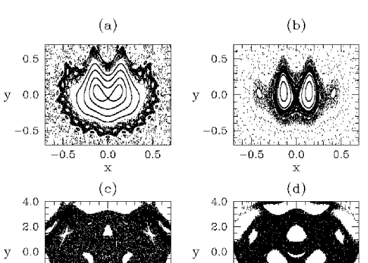
FIG. 1.: Poincaré map for Eq.(2.3) with $\omega=20.1$ (typical of AGB stars) and (a) $\alpha=0.1$, (b) $\alpha=0.4$, and for $\omega\simeq 3$ (typical of Super-AGB stars) and (c) $\alpha=0.1$, (d) $\alpha=0.4$. In all cases, $\epsilon=1$. Note the difference in the scales of the axes.

]

$$\omega_{\rm m}\equiv\Big{(}\frac{GM}{R_{*}^{3}}\Big{)}^{1/2}$$

is the characteristic dynamical frequency of the system and $Q$ the transmission coefficient of the transition zone through which the pressure waves from the interior propagate. In the limit $r\approx 1$ (small oscillations) and absorbing some terms into $t$ as phase shifts, one gets:

$$\frac{d^{2}x}{dt^{2}}=-x+\epsilon\sin[\omega(t-x+\alpha\omega^{-2/3}\sin\omega t)]$$ (8)

where $\epsilon=Q\omega^{4/3}\alpha$ is the total driving amplitude, and $x\equiv r-1$. The parameter $\omega$ is a measure of the core/envelope ratio, and provides information on the location of the source of the driving in the stellar interior. Note that for $\epsilon=0$, Eq.(2.3) transforms into the classical equation of the linear oscillator, $\ddot{x}=-x$. All the interesting features of the motion are generated by the perturbation (the second term of the right-hand side of Eq.(2.3) with $\epsilon\neq 0$) and its interaction with the unperturbed motion. The system we are dealing with is a periodic–time dependent Hamiltonian system.

$$H(x,y;t) = \frac{x^{2}+y^{2}}{2}$$ (10)

$$-\frac{\epsilon}{\omega}\cos[\omega(t-x+\alpha\omega^{-2/3}\sin\omega t)]$$

The associated Poincaré map is an area preserving map. Hence, its dynamics does not exhibit attractors or repellers.

III Characterization of the oscillator

The study performed in [1] explored a limited set of values of the parameter space: $\epsilon=0.5,\,0.75,\,1.0$, and $\alpha=0.1,\,0.2,\,0.4$ for values of $\omega$ around $\simeq 20$, which is characteristic of regular AGB stars ($M\leq 8\,M_{\odot}$). Their main results and conclusions are that small values of $\omega$ produce more strongly chaotic pulsations and that for large values of $\alpha$ stable orbits in some definite regions of the phase space are obtained. Our aim is to extend the previous study to Super-AGB stars, which are characterized by a different value of $\omega$. For the physical conditions found in Super-AGB stars, $8\,M_{\odot}\leq M\leq 11\,M_{\odot}$ and $R_{*}\sim 450\,R_{\odot}$, it turns out that $\omega\mathrel{\mathchoice{\lower 3.6pt\vbox{\halign{$\mathsurround=0pt\displaystyle\hfill#\hfil$\cr>\crcr\sim\crcr}}}{\lower 3.6pt\vbox{\halign{$\mathsurround=0pt\textstyle\hfill#\hfil$\cr>\crcr\sim\crcr}}}{\lower 3.6pt\vbox{\halign{$\mathsurround=0pt\scriptstyle\hfill#\hfil$\cr>\crcr\sim\crcr}}}{\lower 3.6pt\vbox{\halign{$\mathsurround=0pt\scriptscriptstyle\hfill#\hfil$\cr>\crcr\sim\crcr}}}}3$. We will also explore a wider range of the parameter space than that investigated in [1]. Contrary to [1], who adopted a fourth-order predictor-corrector scheme for the numerical integration of Eq.(2.3), we use a fourth order Runge-Kutta integrator with step-size control and dense output as described in [38]. We have tested several other integrators, specifically designed for stiff problems [39], and we have obtained the same results for a given set of initial conditions. Thus we conclude that our numerical integrator is appropriate for problem under study.

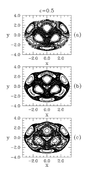
FIG. 2.: The effect of increasing $\alpha$ on the Poincaré map: (a) $\alpha=0.2$; (b) $\alpha=0.3$ and (c) $\alpha=0.4$. $\epsilon=0.5$ in all cases.

A AGB stars vs. Super-AGB stars: the role of $\omega$

In order to compare the behaviour for two different values of $\omega$ (and, thus, the differences between pulsations of AGB and Super-AGB stars), Figure 1 shows the Poincaré maps obtained with $\omega\simeq 20$, typical of regular AGB stars (panels a and b), and those obtained for $\omega\simeq 3$ typical of Super-AGB stars (panels c and d), for the same initial conditions. As $\omega$ increases the behaviour becomes more irregular, and the islands and the structure of panels (a) and (b) quickly disappear, leading to a more chaotic behaviour. Consequently, we expect that the pulsations of Super-AGB stars will exhibit a more chaotic behaviour than those of AGB stars.

The phase portrait of our model is a typical example of an area-preserving map. For very small values of the perturbation parameter, it exhibits invariant circles on which the motion is quasi–periodic. Three periodic island chains surround the fixed point of the map. For large perturbations, because of the breaking–up of the invariant circles and splitting of the separatrices of hyperbolic periodic points, chaotic zones are present, as well as islands in the stochastic sea. Until recently, it was thought that the existence of islands was not very important in determining the origin and character of chaos in Hamiltonian systems. However, it has been recently shown that the boundaries of such islands are very interesting [40, 41, 42]. In particular, crossing an island boundary means a transition from a regular periodic or quasiperiodic behaviour to an irregular one that lies in the stochastic sea. One of the particularities of this singular zone is illustrated in Figure 1a. One can see a central island embedded in the domain of chaotic motion with a boundary separating the area of chaos from the region of regular motion. By changing a control parameter of the system, several bifurcations occur which influence the topology of the boundary zone, leading to the appearance and disappearance of smaller islands. This may result in self-similar hierarchical structures of islands which is crucial for understanding chaotic transport in the stochastic sea and the general dynamics, since they represent high-order resonances.

Figure 1b illustrates another essential phenomenon typical of some Hamiltonian systems. It is linked to the existence of a complex phase space topology in the neighborhood of some islands: a trajectory can spend an indefinitely long time in the boundary layer of the island (i.e., a dynamical trap). The main uncertainty in characterizing this phenomenon concerns the level of stickiness (that is, its characteristic trapping time) which depends on the parameters of the system in a still unknown manner. In general, the hierarchical structure of the islands in the boundary zone can explain the origin of the stickiness of the trajectory within this region, which is the reason why this behaviour is called hierarchical–islands trap [42]. Much attention was generally paid to understanding the structure of these islands because different islands correspond to different physical processes responsible for their origin. The boundary layer of an island may include higher-order resonant islands. Another important reason is that the topology of the islands could be an indicator for the vicinity of bifurcations. However, no general description for the birth and collapse of hierarchical islands exists yet.

[

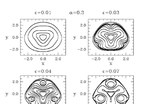
FIG. 3.: Poincaré maps for Eq.(2.3), $\alpha=0.3$ and different values of $\epsilon$. The successive birth of two dimerized island chains. The homoclinic and heteroclinic connections appear in red color.

]

B The role of the fractional driving amplitude, $\alpha$

In order to characterize in depth the behaviour of our system, we have performed a thorough parametric study by varying $\alpha$ and $\epsilon$, while keeping $\omega$ constant at the value typical of Super-AGB stars. Reasonable values of the fractional amplitude, $\alpha$, range from 0.1 to 0.4, whereas the total driving amplitude, $\epsilon$, varies between 0.1 and 1.0. Since $\alpha$ is the ratio between the amplitude of the internal driving and the radius of the star, the upper limit considered in this study is 40%, which is physically sound. In general, a star is characterized by its compactness, $\omega$, and the interior-mantle coupling strength $Q=\epsilon/(\omega^{4/3}\alpha)$, which should stay within the limits of 0 (0$\%$ transmission) and 1 (100$\%$ transmission) in order to maintain its physical meaning. Therefore some specific combinations of $(\epsilon,\alpha)$ that lay outside this range for $Q$ must be regarded with caution, since they have no physical meaning. According to all these considerations, we have investigated the dynamics of the system associated to Eq.(2.3) rewritten below in the form of a perturbed oscillator,

$$\dot{x} = y$$ (11)

$$\dot{y} = -x+\epsilon\sin[\omega(t-x+b\sin\omega t)]$$ (13)

where $b=\alpha\omega^{-2/3}$, maintaining a constant value of $\omega\simeq 3$, as discussed above.

In a first step, we have studied the qualitative changes in the dynamics (i.e., bifurcations) as the parameters $\epsilon$ and $\alpha$ are varied. Poincaré maps corresponding to the case $\alpha\in(0.1-0.4)$ and $\epsilon=0.5$, for several initial conditions, are shown in Figure 2. The maps are characterized by the same geometric structure: a region, centered around $(x,y)=(0,0)$, of closed orbits, surrounded by a region of chaotic orbits. As it can be seen in Figure 2, as $\alpha$ increases, the central region of regular behaviour expands to the detriment of the stochastic sea.

We have also analyzed the behaviour of the system for negative values of $\alpha$. A quick look at the driving allows one to see that negative values of $\alpha$ correspond to a mere change of phase in the driving and, therefore, correspond also to physically meaningful cases. However, and for the sake of clarity and conciseness, in this paper we will concentrate our efforts on the positive domain of this parameter. Nevertheless, we would like to remark at this point that the phase portrait of the Poincaré map changes drastically depending on whether $\alpha$ is positive, negative or almost zero.

[

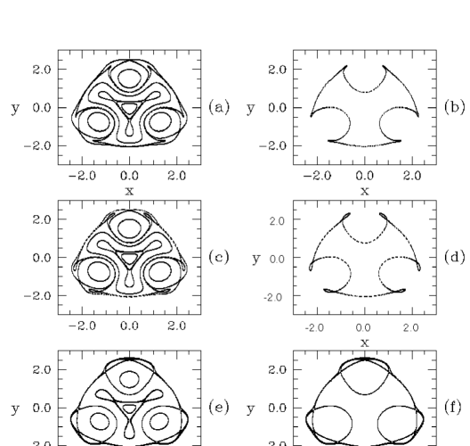
FIG. 4.: Creation by saddle– center bifurcation of a pair of three periodic orbits for $\alpha=0.3$ and increasing values of $\epsilon$. (a): $\epsilon=0.0875$ — the phase portrait at the threshold of the bifurcation; (b): the invariant circle with 6 cusps for the case (a); (c) $\epsilon=0.095$ — two intertwined orbits of period three have been created, inside each new-born loop there is a period three elliptic point; (d): a sequence of heteroclinic and homoclinic connections between the new born hyperbolic points; (e): $\epsilon=0.11725$ — the threshold of global bifurcation; (f): the new topology of the separatrices.

]

C The role of the total driving amplitude, $\epsilon$

Next we have focused on values of $\epsilon\ll 1$ in order to observe in detail the departure of our equation from the harmonic oscillator as this parameter increases. We restricted the study of the Poincaré map to a rectangle limited by initial conditions close to reasonable values of the radius and velocity of the mantle. The restriction is also due to the approximations involved in deriving Eq.(2.3). For $\epsilon=0$ we get an integrable Hamiltonian system, whose integrals of motion are the tori given by the condition $x^{2}+y^{2}=C,~{}t=[0,2\pi/\omega)$. The Poincaré map has the elliptic fixed point (0,0), which corresponds to a periodic orbit of period $P=2\pi/\omega$ of the perturbed Hamiltonian system.

We have chosen the range $\epsilon\in(0,0.12)$ and $\alpha=0.3$ and we have obtained a cascade of local and global bifurcations. Note that the considered pairs of parameters $(\epsilon,\alpha)$ are located above the curve $\alpha^{*}(\epsilon)$, which is the curve of triplication of the elliptic fixed point. According to [43, 44] the corresponding Poincaré map is in these cases a nontwist map. The sequence of detected local and global bifurcations is typical for such a map [45, 46, 47, 48]. Figure 3 illustrates the birth in stages of two dimerized island chains containing periodic points of period three. This is a typical scenario of creation of new orbits in nontwist maps. The upper-left panel exhibits the phase portrait of the near–to–integrable map. The elliptic fixed point is surrounded by invariant circles. At $\epsilon=0.03$ starts the birth of the first dimerized island chain, namely a regular invariant circle bifurcated to an invariant circle with three cusps. The newly born dimerized island chain is clearly seen in the bottom–left panel of the Figure 3, where a new circle with three cusps, closer to the the fixed point can be seen. Both dimerized island chains are illustrated in the bottom–right panel. Between them the invariant circles are meanders. Note that each cusp is a point of saddle–center creation [49]. This scenario is a good example to illustrate the theoretical results concerning the creation of a twistless circle after triplication [43, 44].

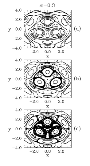
FIG. 5.: Poincaré sections for $\alpha=0.3$ and different values of $\epsilon$: (a) $\epsilon=0.2$; (b) $\epsilon=0.3$, and (c) $\epsilon=0.4$. In red and green colors are represented evolutions of initial conditions close to the first and respectively second separatrix.

Around the last born three–periodic dimerized island chain, a sequence of local and global bifurcations occurs. This is illustrated in Figure 4, where it can be seen that two independent orbits of the same period three are created by cusp bifurcation. They evolve in such a way that, finally, interact with the orbits which belong to the first dimerized island chain. As $\epsilon$ increases the newly born elliptic points approach the hyperbolic points of the dimerized chain. When $\epsilon$ reaches a value of 0.11725 a global bifurcation occurs: the newly created orbits interfere, and the hyperbolic points of the dimerized island chain become hyperbolic points with homoclinic eight-like orbits encircling the new created elliptic points. We have also noticed that as $\epsilon$ increases, the process of creation of three periodic orbits repeats outside the region of the Poincaré map we focus on, and the new orbits form chains of vortices, not dimerized island chains. This behaviour is due to the oscillating character of the nontwist property of the perturbation.

In a second step we have paid attention to larger values of $\epsilon$. In particular we have studied the range $\epsilon\in(0.2,0.5)$. The increase in strength of the external perturbation destroys the separatrices (Figure 5, top) by clothing every one of them in a stochastic layer (Figure 5, middle). As the thickness of the layers increases with the perturbation, depending on the positions of the separatrices in the phase space, they can merge forming the stochastic sea (Figure 5, bottom).

There are many islands, which the chaotic trajectory cannot penetrate. Within an island there are quasiperiodic motions (invariant tori) and regions of trapped chaos. The stronger the chaos is, the smaller the islands and the larger the fraction of phase space occupied by the stochastic sea. The coexistence of regions of regular dynamics (closed orbits) and regions of chaos in the phase space is a wonderful example of the property which differentiates chaotic systems from ordinary random processes, where no stability islands are present. This property makes possible the analysis of the onset of chaos and the appearance of minimal regions of chaos. To summarize, the system undergoes the following bifurcations, as it results from Figures 3, 4 and 5:

1. For $\epsilon\in[0,0.03)$, the phase portrait of the Poincaré map is similar to that of the harmonic oscillator, with the elliptic fixed point $(x,y)=(0,0)$ surrounded by almost circular closed orbits.

2. For $\epsilon\in[0.03,0.04)$, in addition to the central elliptic point, a dimerized island chain is born, namely, three periodic elliptic and hyperbolic points, each elliptic point being surrounded by a homoclinic orbit to the corresponding hyperbolic point, and distinct hyperbolic points being connected by heteroclinic orbits.

3. For $\epsilon\in[0.04,0.07)$, a second dimerized island chain is created, which is a typical configuration after the triplication of an elliptic fixed point.

4. For $\epsilon\in[0.07,0.2)$, a sequence of local and global bifurcations occurs which interphere with the first created dimerized island chain: a regular meander bifurcates to a meander with 6 cusps. A new dimerized island chain is created by saddle–center bifurcation. If we denote the cusps as $1,2,\ldots,6$ in clockwise order, then the elliptic and hyperbolic points born from the odd cusps, form independent orbits of those born from the even cusps. This particular dimerized island chain approaches the original one, and as a result the hyperbolic points of the two chains are connected giving rise to a pattern of a complicated topological type (Figure 4f).

5. For $\epsilon\in[0.2,0.3)$, we notice a more definite chaotic behaviour created by the instability of the remainings of the first heteroclinic orbit engulfing the periodic points of case (c).

6. For $\epsilon\in[0.3,0.5]$, we notice the extension of the chaotic orbits in the central region, together with the continuous generation of pairs of three elliptic fixed points in the outer region as $\epsilon$ increases.

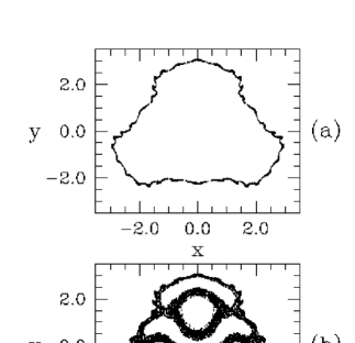
FIG. 6.: (a): A meander near an invariant circle with 35 cusps for $\epsilon=0.4$ and $\alpha=0.3$; (b): two orbits, one filling the meander and the second, a chaotic orbit, confined by the meander.

Another important feature of the phase portrait characteristic of nontwist maps is the existence of meanders (i.e., invariant circles which fold exactly as a meander). Meanders are created between two successively born dimerized island chains, and between two chains of vortices. In twist standard–like maps they become usual circles after the reconnection of the two chains. Note that in our case the reconnection of the first two created dimerized island chains, does not occur, and as $\epsilon$ increases the meanders break–up leaving instead a Cantor set. The top panel of Figure 6 illustrates a meander near a pair of dimerized island chains containing periodic orbits of period 35. Meanders appear to be robust invariant circles, even when the nearby orbits are chaotic (Figure 6, bottom panel). This behaviour was observed in nontwist standard-like maps [47], but until now there is no explanation for this robustness.

IV Comparison with the perturbed oscillator

In order to get a better insight of the underlying physics of the oscillator studied so far, in this section we are going to compare it with the motion of a perturbed oscillator, which has been already studied extensively. This is important since, as it will be shown below, the formal appeareance of Eq.(2.3) does not differ very much from that of a perturbed oscillator. In order to make this clear consider the motion of a perturbed linear oscillator in the form of:

$$\ddot{x}+\omega_{0}^{2}x=\epsilon\sin[\omega x-\omega t]$$ (14)

The left-hand side of Eq.(4.1) describes very simple dynamics of linear oscillations of frequency $\omega_{0}$. To ease the comparison with the perturbed oscillator, Eq.(2.3) can be rewritten as:

$$\ddot{x}+\omega_{0}^{2}x=-\epsilon[\omega x-\omega(t)t],$$ (15)

where

$$\omega(t)=\omega\left(\frac{b\sin\omega t}{t}+1\right)$$ (16)

Both equations share common features. It is important to point out here that for our system $\omega_{0}=1$, as it results from Eq.(2.3). The Hamiltonian associated with the system given by Eq.(4.1) is:

$$H=\frac{(\dot{x}^{2}+\omega_{0}^{2}x^{2})}{2}-\frac{\epsilon}{\omega}\cos[\omega x-\omega(t)t]$$ (17)

Consequently, for weak perturbations the results obtained so far should be similar to the case of a perturbed oscillator. And indeed this is the case, the only difference resides in the period 3 homoclinic orbit, that is in point d) of the summary given in section III.C. The creation of this period-3 homoclinic structure was illustrated in Figure 2 as $\alpha$ increases from $\alpha=0.2$ to $\alpha=0.3$. This suggests that the ultimate reason of this difference might be the presence of the function $\omega(t)$ from Eq.(4.3) as a weak detuning of resonance.

[

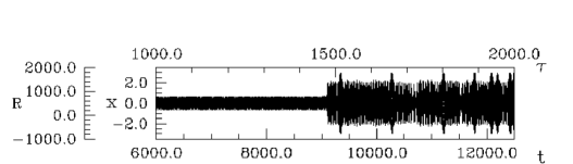
FIG. 7.: Variations of radius (top) and velocity (bottom) as a function of time for $\omega\simeq 3$, $\alpha=0.3$, $\epsilon=0.5$ and the initial condition $(x_{0},y_{0})=(0.0,0.02)$. The escape velocity of the model star ($v_{\rm esc}\simeq 86$ km/s) is represented as a red line.

]

We rewrite Eq.(4.2) with $\alpha\neq 0$ in the following way:

$$\ddot{x}+\omega_{0}^{2}x=\epsilon\sin\omega(t-x+b\sin\omega t)]$$ (18)

For $\alpha=0$, Eq.(4.5) transforms into:

$$\ddot{x}+\omega_{0}^{2}x=\epsilon\sin[\omega(t-x)]$$ (19)

All these ordinary differential equations, together with the well known equation for the perturbed oscillator, have the same mathematical structure. It is an example of weak chaos, where the perturbation itself creates the separatrix network at a certain $\epsilon_{0}$ and then destroys it as $\epsilon$ increases beyond $\epsilon_{0}$ by producing channels of chaotic dynamics. For an unperturbed equation, the unperturbed Hamiltonian $H_{0}$ intrinsically has separatrix structures and the perturbation clothes them in thin stochastic layers, an example of strong chaos. In the phase space there appear invariant curves (deformed tori) embracing the center which do not allow diffusion in the radial direction. Inside these cells of the web, motion occurs along closed-orbits, around the elliptic points from the centers of the cells. With the increase of $\epsilon$ and creation of the stochastic layers, particles can wander along the channels of the newly born web, a phenomenon that represents an universal instability and gives birth to chaotic fluctuations. The heteroclinic structures formed as the perturbation increases through this bifurcation are what differentiates our equation from the typical equations of Hamiltonian chaos and in particular from those of the perturbed oscillator.

V Astrophysical interpretation of the results

In order to provide the reader with a feeling of the physical ranges for the stellar fluctuations in radius and velocity, in Figure 7 we show a particular time series of the model presented above. In this figure the variations of radius and velocity as functions of time are represented both in physical units (solar radii, km/s and years, respectively) and in adimensionalized units — as we have been doing so far.

Generally speaking, the primary information that one can derive from a generic computed or observed time series is the spectral distribution of energies (or amplitudes) of the light curve. We found that for some initial conditions, the resultant time series do not show a single frequency or a small set of frequencies but, in addition, linear combinations of the primary frequencies may also appear in the spectra. This behaviour has been found in real stars quite frequently, and in particular in LPVs, Cepheids and RR Lyrae stars [50].

In any calculation of a time-varying phenomenon, like the one we are describing here, there is always the important practical question of when the simulations should be terminated. For full nonlinear hydrodynamic simulations, even in the case in which a stable limit cycle seems to have set in, one often is worried about the fact that thermal changes, which take place on a longer timescales, could still be occurring. In a recent paper [52], the authors have carried the calculations of Mira variable pulsations much further than in previous investigations and, to their surprise, they have found that the actual behaviour was significantly different from what it was previously thought. To be precise, they obtained a new modified “true” limit cycle which is quite different from the earlier, “false” limit cycle. In agreement with these results, the numerical integration of our system presents a similar behavior, despite the very crude approach adopted here which results in an extreme simplicity of the model. This is shown in Figure 7 for a particular orbit: during the first $\sim 1400$ yr the star oscillates quite regularly, and with small amplitudes. After this period of time, the quiet phase suddenly stops and pulsations become more violent and chaotic. Moreover, at late times the velocity of the outer layers exceeds the escape velocity and, hence, mass loss is very likely to occur, in accordance with the observations of LPVs, which are the observational counterparts of Super-AGB stars.

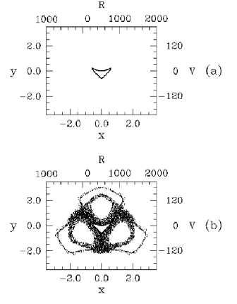
FIG. 8.: Poincaré map for the orbit of Figure 7. Panel (a) includes the points $R(\tau)$ and $V(\tau)$ for the time interval (1000-1400) years, whereas panel (b) shows the points $R(\tau)$ and $V(\tau)$ for the time interval (1000-2000) years.

This behaviour — a quiet phase, followed by an extremely violent phase — is a typical case of a dynamical trap discussed in section III. The Poincaré map associated with the radius and velocity variations in Figure 7 is shown in Figure 8. None of these figures include the oscillations previous to 1000 years because the behaviour is similar to the one of the time interval between 1000 and 1400 years. This example corroborates the suggestion, first proposed by [53] and later found in the very detailed numerical calculations of [52] that the long-term effects in Mira variables have an important role in our understanding of the mechanism which drives mass-loss. This result also argues in favour of the capability of simple models to capture the underlying dynamics of the physical system. To put it in a different way, our model, despite its simplicity, reproduces reasonably well the results obtained with full, sophisticated and nonlinear hydrodynamic models. It is nevertheless important to realize here that our model does not incorporate the secular effects induced by the thermal changes and, hence, it is quite likely that this kind of behaviour is intrinsically associated with the physical characteristics of the oscillations of real stars.

In order to get a more precise physical insight a time-frequency analysis would be very valuable. Consequently we devote the remaining of this section to such a purpose. Most often, astronomers have used wavelet transforms in their investigations of the time-frequency characteristics of variable light curves. However, [54] compared the results obtained with different time-frequency methods using both real light-curves and synthetic signals. From these tests they firstly concluded that the Gábor transform [55] provides much more informative results on the high frequency part of the data than the wavelet transform, but, on the contrary, they also found that the time-frequency analysis using the Choi-Williams distribution [56] is definitely superior to both methods (at least on the data they used). Further investigations carried out by the same authors [51] led them to conclude that in general one cannot claim a priori that any of these methods is better than the others. In fact, this depends largely on the nature of the signal and on which kind of features one tries to enhance. Therefore, it is always advantageous to use simultanously several of them. However, as the Choi-Williams distribution is generally accepted to be the most useful among all the methods, we will center our analysis using this tool, as it was done in [51].

The time-frequency analysis of a model computed with $\omega\simeq 3$, $\alpha=0.3$, $\epsilon=0.5$ and the initial condition $(x_{0},y_{0})=(0.0,0.02)$, is shown in the central panel of Figure 9. In order to be used as a visual help this time series has been reproduced in the bottom panel of this figure. We have split the time series into two pieces, in order to better illustrate the stickiness of the oscillator, and we have computed the Fourier transforms of both pieces separately. These Fourier transforms are shown in the top panels of Figure 9, the left one corresponds to $\tau<1400$ yr, whereas the right one corresponds to $\tau\geq 1400$ yr. Note the difference in the scales of the power, which is much larger for the right panel. As it can be seen in these panels the power is suddenly shifted from relatively large frequencies to much smaller frequencies.

[

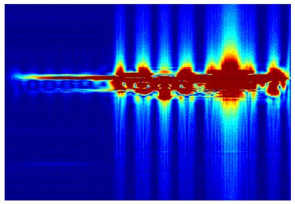
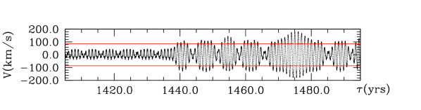
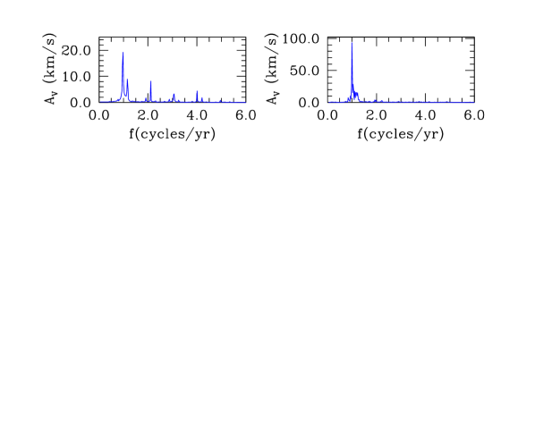
FIG. 9.: Choi-Williams distribution of the velocity variations (central panel), Fourier analysis for $\tau<1440$ yr (top left panel) and for $\tau\geq 1440$ yr (top right panel), and the corresponding time series (bottom panel).

]

This behavior is even more clearly shown in the Choi-Williams distribution. Note as well the contribution of the frequency $f\simeq 2.1$ yr^-1 at small times, just before the beginning of the burst (at $\tau\leq 1430$ yr). Indeed, this small contribution could be at the origin of the transfer of power to $f\simeq 1.2$ yr^-1, which occurs inmediately after $\tau\simeq 1430$ yr and which ultimately leads to the burst at $\tau\simeq 1440$ yr. Also remarkable is the small time elapsed since the beginning of the transfer of power, which is only about 10 yr.

VI Conclusions

We have presented and analyzed the complex dynamics of a forced oscillator which is interesting not only from the mathematical point of view, but also because it describes with a reasonable degree of accuracy the main characteristics of some stellar oscillations. This model has been previously used to study the irregular pulsations of Asymptotic Giant Branch stars [1], and we have used it to study the pulsations of more massive and luminous stars, the so-called Super-Asymptotic Giant Branch stars. In doing this we have extended the previous studies to a range of the parameters specific for this stellar evolutionary phase. We have found, in agreement with the observations of Long Period Variables which are the observational counterparts of Super-Asymptotic Giant Branch stars, that the oscillator shows a chaotic behavior. It is important to realize as well that this kind of stars shows a more pronounced chaotic behavior than regular Asymptotic Giant Branch stars of smaller mass and luminosity. We have also characterized in depth the full sequence of bifurcations as the physical parameters of the model are varied. We have found a rich set of local and global bifurcations which were not described in [1]. Among these, perhaps the most important one is a tripling bifurcation, but meandering curves, hierarchical islands traps and sticky orbits also appear. Correspondingly, the resulting time series also show a rich behaviour. In particular, we have found that although there are light curves which show a rather regular behaviour for certain values of the parameters of the physical system and given initial conditions, there are as well some other light curves which show clear beatings or linear combinations of two main frequencies up to terms of $2f_{0}+7f_{1}$, being $f_{0}$ the fundamental frequency and $f_{1}$ that of the first overtone, and even more complex orbits. For the parameters and initial conditions leading to more irregular behaviour, we noticed the existence of both clear chaotic pulsations and sudden changes from a limit-cycle to chaotic pulsations, the latter being associated with the stickiness phenomenon characteristic of some Hamiltonian systems. For these orbits the velocity of the very outer layers clearly exceeds the escape velocity. Hence, for these chaotic pulsations mass-loss is very likely to occur, in good agreement with the observations, which correlate the degree of irregularity with the mass-loss rate. Regarding the stickiness of some orbits which we have found for a set of parameters, perhaps the most important result is that the long-term effects found in real stars are reproduced by our model, despite of its simplicity, even though the driven oscillator studied here does not incorporate the effects of secular changes. Hence it is quite likely that this kind of behaviour which has been already found in full hydrodynamical simulations [52], is intrinsically associated with the physical characteristics of the oscillations of real stars and not to the long-term thermal changes.

- [1] V. Icke, A. Franck, H. Heske, Astron. & Astrophys., 258, 341 (1992)
- [2] A. Gautschy, H. Saio, Annu. Rev. Astron. & Astrophys., 34, 551 (1996)
- [3] J.P. Cox, Theory of Stellar Pulsation, Princeton Univ. Press: Princeton (1980)
- [4] J.R. Buchler, Astrophys. & Space Sci., 210, 9 (1993)
- [5] A. Gautschy, H. Saio, Annu. Rev. Astron. & Astrophys., 33, 113 (1995)
- [6] J.R. Buchler, Z. Kolláth, R. Cadmus, in Proceedings of the 6th Experimental Chaos Conference, astro-ph/0106329 (2001)
- [7] K. Pollard, C. Alcock, D.R. Alves, D.P. Bennett, K.H. Cook, S.L. Marshall, D. Minniti, R.A. Allsman, T.S. Axelrod, K.C. Freeman, B.A. Peterson, A.W. Rodgers, K. Griest, J.A. Guern, M.L. Lehner, M. L., A. Becker, M.R. Pratt, P.J. Quinn, W. Sutherland, D.L. Welch, in Variable Stars and the Astrophysical Returns of Microlensing Surveys, Eds.: R. Ferlet, J.P. Maillard and B. Raban, Editions Frontiérs: Paris, p. 219 (1997)
- [8] J. Perdang, in The Numerical Modelling of Nonlinear Stellar Pulsation, Ed.: J.R. Buchler, Kluwer: Dordrecht, p. 333 (1990)
- [9] S. Höfner, U.G. Jorgensen, R. Loidl, B. Aringer, Astron. & Astrophys., 340, 497 (1998)
- [10] S. Höfner, Astron. & Astrophys., 346, L9 (1999)
- [11] J.M. Winters, T. Le Bertre, K.S. Jeong, Ch. Helling, E. Sedlmayr, Astron. & Astrophys., 361, 641 (2000)
- [12] Y.J.W. Simis, V. Icke, C. Dominik, Astron. & Astrophys., 371, 205 (2001)
- [13] G. Bono, M. Marconi, R.F. Stellingwerf, Astron. & Astrophys., 360, 245 (2000)
- [14] C. Ritossa, E. García-Berro, I. Iben, Astrophys. J., 460, 489 (1996)
- [15] E. García-Berro, C. Ritossa, I. Iben, Astrophys. J., 485, 765 (1997)
- [16] D. Barthes, Astron. & Astrophys., 333, 647 (1998)
- [17] D. Barthes, X. Luri, R. Alvarez, M.O. Mennessier, Astron. & Astrophys. Suppl. Ser., 140, 55 (1999)
- [18] J.P. Norris, R.J. Nemiroff, J.D. Scargle, C. Kouveliotou, G.J. Fishman, C.A. Meegan, W.S. Paciesas, J.T. Bonnel, Astrophys. J., 424, 540 (1994)
- [19] J. Hjorth, Astrophys. J., 424, 106 (1994)
- [20] E. Slezak, F. Durret, D. Gerbal, Astron. J., 108, 1996 (1994)
- [21] M.J. Goupil, M. Auvergne, A. Baglin, Astron. & Astrophys., 250, 89 (1991)
- [22] J.R. Buchler, G. Kóvacs, Astrophys. J., 320, L57 (1987)
- [23] G. Kóvacs, J.R. Buchler, Astrophys. J,. 334, 971 (1988)
- [24] T. Aikawa, Astrophys. & Space Sci., 164, 295 (1990)
- [25] J.R. Buchler, M.J. Goupil, G. Kóvacs, Phys. Lett. A, 126, 177 (1987)
- [26] T. Aikawa, Astrophys. & Space Sci., 139, 281 (1987)
- [27] T. Serre, Z. Kolláth, J.R. Buchler, Astron. & Astrophys., 311, 833 (1996)
- [28] J.R. Buchler, T. Serre, Z. Kolláth, Phys. Rev. Lett., 74, 842 (1995)
- [29] Z. Kolláth, J.R. Buchler, T. Serre, J. Mattei, Astron. & Astrophys., 329, 147 (1998)
- [30] N. Baker, in Stellar Evolution, Eds.: R.F. Stein and A.G.W. Cameron, Plenum Press: New York, p. 333 (1966)
- [31] N. Baker, D. Moore, E.A. Spiegel, Astron. J., 71, 845 (1966)
- [32] T.J. Rudd, R.M. Rosenberg, Astron. & Astrophys. 6, 193 (1970)
- [33] R.F. Stellingwerf, Astron. & Astrophys., 21, 91 (1972)
- [34] J.R. Buchler, O. Regev, Astrophys. J., 263, 312 (1982)
- [35] Y. Tanaka, M. Takeuti, Astrophys. & Space Sci., 148, 229 (1988)
- [36] M. Saitou, M. Takeuti, Y. Tanaka, Publ. Astron. Soc. Pac., 41, 297 (1989)
- [37] W. Unno, D.-R. Xiong, Astrophys. & Space Sci., 210, 7 (1993)
- [38] E. Hairer, S.P. Norsett, G. Wanner, Solving Ordinary Differential Equations, Nonstiff Problems, Springer-Verlag: Berlin (1993)
- [39] L. Shampine, M. Gordon, Computer Solution of Ordinary Differential Equations, Freeman: San Francisco (1975)
- [40] G.M. Zaslavsky, Phys. Today, 52, 39 (1999)
- [41] G.M. Zaslavsky, M. Edelman, B.A. Niyazov, Chaos, 7, 159 (1997)
- [42] G.M. Zaslavsky, Physics of chaos in Hamiltonian systems, Imperial College Press: London (1998)
- [43] H.R. Dullin, J.D. Meiss, D. Sterling, Nonlinearity, 13, 203 (2000)
- [44] V.I. Arnold, V.V. Kozlov, A.I. Neishtadt, Dynamical Systems III, Springer-Verlag: Berlin (1988)
- [45] D. del-Castillo-Negrete, J.M. Greene, P.J. Morrison, Physica D, 91, 1 (1996)
- [46] D. del-Castillo-Negrete, J.M. Greene, P.J. Morrison, Physica D, 100, 311 (1997)
- [47] C. Simó, Regular and Chaotic Dynamics, 3, 180 (1998)
- [48] E. Petrisor, submitted to Nonlinearity (2002)
- [49] J. K. Hale, H. Kocak, Dynamics and bifurcations, Springer-Verlag: Berlin (1991)
- [50] Z. Kolláth, J.R. Buchler, in Stellar Pulsation – nonlinear studies, Eds: M. Takeuti & D. Sasselov, Kluwer: Dordrecht, p. 29 (2001)
- [51] J.R. Buchler, Z. Kolláth, in Stellar Pulsation – nonlinear studies, Eds: M. Takeuti & D. Sasselov, Kluwer: Dordrecht, p. 185 (2001)
- [52] A. Ya’ari, Y. Tuchman, Astrophys. J., 456, 350 (1996)
- [53] J.R. Buchler, W.R. Yueh, J. Perdang, Astrophys. J., 214, 510 (1977)
- [54] Z. Kolláth, J.R. Buchler, in Nonlinear Signal and Image Analysis, Eds: J.R. Buchler and H. Kandrup, New York Academy of Sciences Press: New York, 808, p. 116 (1997)
- [55] D. Gabor, J. Inst. Elec. Eng., 93, 429 (1946)
- [56] H.I. Choi, W.J. Williams, IEEE Trans. on Acoust. Speech and Signal Processing, 37, 862 (1989)