Evolution of the X-ray Properties of Clusters of Galaxies

Abstract

The amount and nature of the evolution of the X-ray properties of clusters of galaxies provides information on the formation of structure in the universe and on the properties of the universe itself. The cluster luminosity - temperature relation does not evolve strongly, suggesting that the hot X-ray gas had a more complicated thermodynamic history than simply collapsing into the cluster potential well. Cluster X-ray luminosities do evolve. The dependence of this evolution on redshift and luminosity is characterized using two large high redshift samples. Cluster X-ray temperatures also evolve. This evolution constrains the dark matter and dark energy content of the universe as well as other parameters of cosmological interest.

Institute for Astronomy, University of Hawaii, 2680 Woodlawn Drive, Honolulu, HI 96822, USA

1. Introduction

The evolution of cosmic structure is strongly dependent on the cosmology of the universe. Jenkins et al. (1998) is one of the many papers describing this well known result. Clusters of galaxies, as the most massive bound objects known, are the ultimate manifestations of cosmic structure building. The evolution of clusters is simple, being driven by the gravity of the underlying mass field of the universe and of a collisionless collapse of cluster dark matter. It should be possible to calculate this evolution reliably compared to that of other objects visible at cosmological distances such as galaxies or AGN. Clusters are luminous X-ray sources. The X-ray emission mechanism is optically thin thermal radiation from a medium nearly in collisional equilibrium, about the simpliest situation imaginable. Thus observations of the X-ray evolution of clusters provide a robust measure of the evolution of cosmic structure and thereby constrain the cosmology of the universe.

The cosmological model is described by a set of cosmological parameters. The present value of the Hubble parameter is $\mathrm{H_{0}\equiv 100\>h\>km\>s^{-1}\>Mpc^{-1}}$. When needed h = 0.5 will be used, but almost nothing about evolution depends on the precise value of h since data at two epochs are always compared. The present matter and dark energy densities in terms of the critical density are $\Omega_{m0}$ and $\Omega_{\Lambda 0}$ respectively. The amount of structure in the universe is described by $\sigma_{8}$, the present rms matter fluctuations in spheres of $\mathrm{8\>h^{-1}\>Mpc}$. This parameter is a complicated way to describe the present normalization of the spatial power spectrum of matter density fluctuations, P(k), on a scale of k $\sim\>0.2\mathrm{\>h\>Mpc^{-1}}$: $\mathrm{\sigma_{8}\approx[P(0.172\>h\>Mpc^{-1})/3879\>h^{-3}\>Mpc^{3}]^{1/2}}$ (Peacock, 1999 equations 16.13 and 16.132). The dark energy equation of state is P = w $\rho$ c². If w = -1, then the dark energy is the cosmological constant, if $\mathrm{-1<w<0}$ it is termed Quintessence. Recall that w = 0 is cold dark matter and w = 1/3 is radiation. Cluster temperature evolution provides constraints on all of the above cosmological parameters except h.

When needed, two specific cases will be considered. The X-ray astronomer’s universe where $\Omega_{m0}=1.0,\Omega_{\Lambda 0}=0.0$. This combination was known to be correct ten years ago. The other case may be called the bandwagon universe where $\Omega_{m0}=0.3,\Omega_{\Lambda 0}=0.7$. This combination is known to be correct today. Both universes are spatially flat, $\Omega_{m0}+\Omega_{\Lambda 0}=1$.

2. Cluster Luminosity - Temperature Relation Evolution

The relation between cluster X-ray luminosities and temperatures (L - T relation) is the oldest and best studied among cluster X-ray observables. Early studies include Mitchell, Ives & Culhane (1977), Mushotzky et al. (1978) and Henry & Tucker (1979). Recent comprehensive work includes David et al. (1993), White, Jones & Forman (1997), Markevitch (1998) and Arnaud & Evrard (1999). Figure 1 shows an example of this relation using a sample of 53 $z<0.3$ and 32 $0.3\leq z\leq 0.6$ clusters all with ASCA temperatures (Novicki, Sornig, & Henry, 2002).

Figure 1.: The cluster luminosity - temperature relation. Triangles are the low redshift sample and squares are the high redshift sample. The line is the best fit to the entire sample of $L(bol)=C[kT]^{\alpha}(1+z)^{A}$. a. (left) For a cosmology with $\Omega_{m0}=1.0,\Omega_{\Lambda 0}=0.0$. b. (right) For a cosmology with $\Omega_{m0}=0.3,\Omega_{\Lambda 0}=0.7$.

Although there is clearly a relation in Figure 1, there is also substantial non-statistical scatter. The scatter is approximately Gaussian distributed in the logarithm of the luminosity at constant temperature. The dispersion in the logarithm of the bolometric luminosity, $\mathrm{\sigma logL(bol)}$, is about 0.2. The scatter is reduced if the effects of the cluster cooling centers are removed, either by modeling them (Allen & Fabian, 1998), excising them (Markevitch, 1998), or only using clusters that do not have cooling centers (Arnaud & Evrard, 1999).

Most observers adopt the simple functional form $L(bol)=C[kT]^{\alpha}(1+Z)^{A}$, where $L(bol)$ is the bolometric luminosity, to describe their results. The observations indicate that $\alpha\sim 3$. However, simple scaling relations predict $\alpha=2$ and $A=1.5$. This $\alpha$ discrepancy is usually resolved by positing that the cluster gas has experienced some form of preheating prior to its heating through gravitational collapse (Evrard & Henry, 1991; Kaiser, 1991; Bialek, Evrard, & Mohr 2001; Tozzi & Norman, 2001; Bower et al., 2001). Preheating raises the temperatures of low mass clusters more than those of high mass, thereby breaking the scaling relations. These preheating models predict little or no evolution of the L - T relation, at least to redshifts $\sim 1$. For example, the model in Evrard & Henry (1991) has $\alpha=2.5$ and $A=0$. An alternative to this idea invokes cooling, which is more efficient at lower temperatures, and a small amount of post collapse heating to break the scaling (Voit & Bryan, 2001). Little evolution is expected in this model as well. Thus the values of $\alpha$ and $A$ provide clues to the thermodynamic history of the cluster gas.

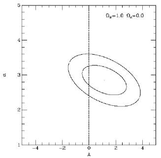
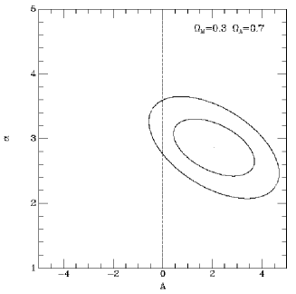
Figure 2.: The 1 and 2 $\sigma$ contours for a fit of the data in Figure 1 to $L(bol)=C[kT]^{\alpha}(1+z)^{A}$. a. (left) For a cosmology with $\Omega_{m0}=1.0,\Omega_{\Lambda 0}=0.0$. b. (right) For a cosmology with $\Omega_{m0}=0.3,\Omega_{\Lambda 0}=0.7$.

It has recently become possible to constrain the evolution of the L - T relation, thereby testing these scenarios. Figure 2 shows the constraints derived by Novicki et al. (2002). The evolution is mild; A is consistent with 0 at the $\sim 1\sigma$ level. Similar results have been found by Henry, Jiao, & Gioia (1994), Mushotzky & Scharf (1997), Sadat et al. (1998), Donahue et al. (1999), Reichart, Castander & Nichol (1999), Fairley et al. (2000), and Arnaud, Aghanian & Neumann (2002). Little or no evolution may then imply that the thermodynamic history of cluster gas is more complicated than simply falling into the cluster potential well, at least for low mass clusters. There was possibly some additional heating prior to collapse and/or cooling after collapse.

3. Cluster X-ray Luminosity Evolution

The initial claim for cluster X-ray luminosity evolution was made over a decade ago by Gioia et al. (1990) and Henry et al. (1992) using the Einstein Extended Medium Sensitivity Survey (EMSS). The reported evolution was in the sense that there are fewer high luminosity clusters in the past. This conclusion has not enjoyed universal acceptance. However, there are now many new samples of clusters, both at high and low redshift, with which it may be tested.

3.1. Cluster X-ray Luminosity Samples

Clusters are not standard luminosity candles. Therefore, searching for luminosity evolution requires measuring the X-ray luminosity function at two epochs and that requires constructing statistically complete samples at the two epochs. Fortunately, measuring the X-ray luminosity is relatively easy. It only requires $\sim 25$ photons for a $5\sigma$ luminosity measurement, so large samples are possible with relatively modest observing time.

Table 1.: Low Redshift Cluster Luminosity Samples

Name	Num	Sky Cut	F(0.1,2.4)(cgs)	$\Omega$(deg2)	Reference
BCS	201	$\delta>0.0$	$>4.4\times 10^{-12}$	13,578	Ebeling et al. (1998)
		$\mid b\mid>20$
REFLEX	441	$\delta<2.5$	$>3.0\times 10^{-12}$	13,924	Böhringer et al. (2001)
		$\mid b\mid>20$

Table 1 gives some properties of low redshift (here defined as $z<0.3$) statistically complete cluster luminosity samples. Not included in Table 1 are the RASS1 Bright Sample (De Grandi et al., 1999), which is a subsample of REFLEX and the eBCS sample (Ebeling et al., 2000), which adds another 100 clusters at $\mathrm{F}(0.1,2.4)>2.8\times 10^{-12}$ $\mathrm{e}rg\>cm^{-2}\>s^{-1}$ to the BCS but is 75% complete. The REFLEX sample was constructed from the second (i.e. fully merged) processing of the ROSAT All-Sky Survey (RASS2).

Table 2.: High Redshift Cluster Luminosity Samples

Name	Num	Sky Cut	F(0.5,2.0)(cgs)	$\Omega$(deg2)	Reference
EMSS	22	$\delta>-40$	$>4.6\times 10^{-14}$	778	Gioia & Luppino (1994)
		$\mid b\mid>20$
MACS	119	$\delta<80$	$>6.2\times 10^{-13}$	22,735	Ebeling et al. (2001)
		$\delta>-40$
		$\mid b\mid>20$
NEP	19	$\alpha=18$	$>2.2\times 10^{-14}$	81	Henry et al. (2001)
		$\delta=66.5$
160 deg2	73	$\mid b\mid>20$	$>1.3\times 10^{-14}$	158	Vikhlinin et al. (1998)
RDCS3	50	$\mid b\mid>20$	$>3.0\times 10^{-14}$	47	Rosati (2001)
BSHARC	12	$\mid b\mid>20$	$>1.6\times 10^{-13}$	179	Romer et al. (2000)
WARPS II	78	$\mid b\mid>20$	$>6.0\times 10^{-14}$	73	Jones et al. (2001)

Table 2 gives some properties of the high redshift cluster luminosity samples. Note that most of these samples also have low redshift objects, but only the numbers of $z>0.3$ objects are listed in the table. The EMSS sample is from Einstein Observatory observations, the other samples are from ROSAT. The MACS and NEP samples come from the RASS2, i.e. they are contiguous, all other samples are from disjoint targeted observations with a region around the target excised.

Typically, low redshift cluster samples contain several hundred X-ray bright objects coming from one-third of the sky. High redshift samples usually contain several tens of faint objects coming from less than one-percent of the sky.

3.2. Test For Cluster X-ray Luminosity Evolution In Seven High Redshift Samples

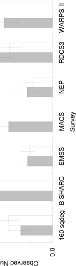
Figure 3.: Ratio of the observed to no-evolution expectation numbers of clusters for seven high redshift surveys. The grey bar assumes $\Omega_{m0}=1.0$, $\Omega_{\Lambda 0}=0.0$; the clear bar $\Omega_{m0}=0.3$, $\Omega_{\Lambda 0}=0.7$. The ratio can not yet be made for MACS and WARPS II for the latter case because the individual cluster luminosities and redshifts are not yet published.

Since the evolution appears to be a lack of objects at high luminosities, simply comparing the binned low and high redshift differential luminosity functions will not use the full statistical power of the sample. In the limit that the evolution is a downward step function above a certain luminosity, such a comparison will show no difference between the two epochs (unless upper limits are plotted).

A more sensitive test is to compare the observed number of high-redshift, high-luminosity clusters to the expected number if the low redshift luminosity function did not evolve. This test accounts for clusters that could have been found but were not.

Specifically, the test used here compares the number of observed clusters with luminosities in the 0.5 - 2.0 keV band $\geq 2\times 10^{44}$ $\mathrm{erg\>s^{-1}}$ (except MACS, whose selection function limits the lowest luminosity to $2.9\times 10^{44}$$\mathrm{erg\>s^{-1}}$) and with $0.3\leq z\leq 1.0$ to the expected number assuming the REFLEX low redshift luminosity function did not evolve. Each of the seven high redshift samples probes a different region of the L - z plane due to its different flux limit and solid angle. The average redshift and luminosity of the clusters after the above cuts for all seven samples is 0.495 and $4.7\times 10^{44}$ $\mathrm{erg\>s^{-1}}$ respectively ($\Omega_{m0}=1.0$, $\Omega_{\Lambda 0}=0.0$). Figure 3 summarizes the results. All seven samples show evolution, most at a statistically significant level. The average ratio of the observed to no-evolution numbers is $0.35\pm 0.04$ for $\Omega_{m0}=1.0$, $\Omega_{\Lambda 0}=0.0$, and $0.29\pm 0.04$ for $\Omega_{m0}=0.3$, $\Omega_{\Lambda 0}=0.7$.

Figure 4.: Ratio of the observed to no-evolution expectation numbers of clusters for the low redshift components of five high-redshift surveys. The sample definition is L(0.5,2.0) $\geq 10^{43}$ $\mathrm{erg\>s^{-1}}$ and $0.15\leq z\leq 0.30$. The grey bar assumes $\Omega_{m0}=1.0$, $\Omega_{\Lambda 0}=0.0$; the clear bar $\Omega_{m0}=0.3$, $\Omega_{\Lambda 0}=0.7$.

Figure 3 also shows that one systematic effect, the assumed cosmology, is not important. Another systematic effect is the choice of the low-redshift luminosity function. Using the BCS instead of REFLEX yields a ratio of $0.38\pm 0.04$ for $\Omega_{m0}=1.0$, $\Omega_{\Lambda 0}=0.0$ (the BCS investigators only gave results for this cosmology). Thus the choice of the low-redshift comparison luminosity function is also not important. The final systematic investigated was whether the test yields a null result, a ratio of 1, at low redshift. Figure 4 shows that it does. The average ratio of the observed to no-evolution numbers is $1.03\pm 0.08$ for $\Omega_{m0}=1.0$, $\Omega_{\Lambda 0}=0.0$, and $0.87\pm 0.08$ for $\Omega_{m0}=0.3$, $\Omega_{\Lambda 0}=0.7$. This test is limited to five samples because the selection function for Bright SHARC has not been published at low redshift and MACS does not attempt to be complete at low redshift.

These results show that there is no longer a question of whether cluster X-ray luminosities evolve, they do. Seven nearly independent surveys show some evolution with a combined significance $>15\sigma$. Systematic effects do not appear to be important. The amount of evolution is about a factor of three at $L(0.5,2.0)\sim 4.7\times 10^{44}$ $\mathrm{erg\>s^{-1}}$ over the redshift range $\sim 0.1$ to $\sim 0.5$. It is now time to better characterize the evolution.

3.3. Characterizing Cluster Luminosity Evolution Using Two Large High Redshift Samples

Figure 5.: X-ray luminosity functions from the low-redshift REFLEX (from Böhringer et al., 2002) and combined EMSS, NEP and 160 deg² high-redshift samples. The figure assumes $\Omega_{m0}=1.0$, $\Omega_{\Lambda 0}=0.0$.

The first large sample comes from combining the 160 deg², EMSS and NEP samples, denoted HEN. There are 109 objects with L(0.5,2.0) $\geq 1\times 10^{43}$ $\mathrm{e}rg\>s^{-1}$ and $0.3\leq z\leq 0.85$. This size is comparable to the low-redshift samples. There are no clusters in common among the three samples and the overlap of their survey regions on the sky is small, only $\sim 5\%$, which has been accounted for statistically. The HEN sample is large enough that a simple comparison of the luminosity functions from it and REFLEX demonstrates the evolution clearly, as Figure 5 shows. A Schechter function fits both the REFLEX and HEN samples well. Figure 6 gives the 1, 2 and 3 $\sigma$ contours for the slope and characteristic luminosity, again demonstrating evolution at high statistical confidence. At least the Schechter function normalization and slope are evolving, but the charcteristic luminosity may not be. Comparison of HEN with REFLEX shows a factor of 2 evolution at L(0.5,2.0) $=2\times 10^{44}$ $\mathrm{erg\>s^{-1}}$ over the redshift interval 0.11 to 0.45 ($\Omega_{m0}=1.0$, $\Omega_{\Lambda 0}=0.0$).

Figure 6.: The 1, 2 and 3$\sigma$ contours for the slope and characteristic luminosity of individual Schechter function fits to the REFLEX and HEN samples. a. (left) For a cosmology with $\Omega_{m0}=1.0,\Omega_{\Lambda 0}=0.0$. b. (right) For a cosmology with $\Omega_{m0}=0.3,\Omega_{\Lambda 0}=0.7$.

It is the nature of flux-limited samples that different luminosity objects are predominately found at different redshifts. Thus the luminosity functions in Figure 5 do not refer to unique epochs. This situation may be overcome to some extent by fitting to an evolving luminosity function, termed the AC model. The AC model generalizes the Schechter funtion to: $\mathrm{n(L,z)=n_{0}(z)L^{-\alpha(z)}exp(-L/L^{*})}$, with $\mathrm{n_{0}(z)=n_{0}(1+z)^{A}}$ and $\mathrm{\alpha(z)=\alpha_{0}(1+z)^{C}}$. A maximum likelihood fit of the AC model to the unbinned luminosity and redshift pairs for the REFLEX and HEN clusters gives the following: $\mathrm{n_{0}=4.65^{+0.58}_{-0.64}\times 10^{-7}Mpc^{-3}(10^{44}erg\>s^{-1})^{\alpha-1}}$, $\mathrm{L^{*}=6.86^{+4.59}_{-1.96}\times 10^{44}erg\>s^{-1}}$, $\alpha_{0}=-(1.70^{+0.15}_{-0.13})$, A = -(1.17 $\pm$ 0.84), C = 0.90${}^{+0.60}_{-0.35}$ ($\Omega_{m0}=1.0$, $\Omega_{\Lambda 0}=0.0$). The errors are at 68% confidence for 4 parameters with the error on $\mathrm{n_{0}}$ determined from letting the errors on the other 4 parameters take their extreme values. Figure 7 gives the best fitting AC luminosity functions, now at two particular epochs.

Figure 7.: Best fitting AC model luminosity functions. The solid line is z = 0.0, while the dashed line is z = 0.5. The figure assumes $\Omega_{m0}=1.0$, $\Omega_{\Lambda 0}=0.0$.

The second large high redshift sample is the Massive Cluster Survey or MACS. This survey seeks a large sample of high luminosity clusters at high redshift. About 300 objects are expected if there is no evolution. Presently the survey is $\sim 90\%$ complete and has 119 clusters. Note that in Section 3.2 an additional $10\%$ systematic error has been added in quadrqture to the MACS statistical errors.

Figure 8.: A nonparametric description of X-ray cluster luminosity evolution detected in the eBCS/MACS samples. The integral luminosity function is shown as a function of redshift. Strictly speaking, the MACS results are lower limits, but the estimated completeness of this survey is $\sim 90\%$. Also shown is the AC model with its $1\sigma$ error band. There are no adjustable parameters used to fit the AC model to the eBCS/MACS. The figure assumes $\Omega_{m0}=1.0$, $\Omega_{\Lambda 0}=0.0$.

A final sample of $\sim 130$ objects means that MACS detects evolution also at high significance. Figure 8 shows a nonparametric representation of this evolution, comparing the MACS and eBCS integral luminosity functions. The comparisons in Section 3.2 folded a model fit to the REFLEX luminosity function through each survey selection function. MACS finds a factor of $\sim 10$ evolution at L(0.1,2.4) $>10^{45}$ $\mathrm{erg\>s^{-1}}$ over the redshift interval 0.05 to 0.55 ($\Omega_{m0}=1.0$, $\Omega_{\Lambda 0}=0.0$). Figure 8 also shows that the AC model fits the MACS data well, with no adjustable parameters and with few clusters in common between eBCS/MACS and REFLEX/HEN.

Two high statistics, high redshift samples agree on the amount and nature of cluster X-ray luminosity evolution. The previous apparent disagreements were probably just poor statistics.

3.4. Constraining Cosmology From Cluster Luminosity Evolution

Given the discussion in the Introduction, the question naturally arises whether cluster luminosity evolution may be used to determine the cosmology of the universe. The difficulty is the extra evolution experienced by the gas in addition to that driven by gravity, as the L - T relation shows. Since X-ray luminosity is proportional to the square of the gas density, will this extra evolution be large enough to mask that from gravity? The weak evolution of the L - T relation shows that the extra evolution occured before what is currently observable, possibly allowing a simple correction. Comparing data to a theory that incorporates the observed L - T (or L - M) relation into the gravitational evolution predictions has in fact been used to constrain cosmological parameters from cluster luminosities (eg Henry et al., 1992; Borgani et al., 2001; Viana, Nichol & Liddle, 2002).

4. Cluster X-ray Temperature Evolution

Perhaps a cleaner way to measure the evolution of cosmic structure using X-ray observations of clusters is via cluster temperature evolution. The temperature is more likely to reflect better the underlying gravity driven evolution than the luminosity.

4.1. Cluster X-ray Temperature Samples

Clusters are not standard temperature temperature baths. Just as with luminosity evolution, measuring temperature evolution requires constructing temperature functions at two epochs. Again, statistically complete samples are required at the two epochs. However it is substantially more difficult to measure cluster temperatures than luminosities. At least 1000 photons are required to provide a reasonable temperature measurement. Obtaining large samples is difficult. Obtaining even two independent samples at high redshift has so far not been possible. Table 3 gives some properties of cluster temperature samples. The last column of the table gives the numbers of clusters with measured temperatures from ASCA and with temperatures estimated from the L - T relation.

Table 3.: Cluster Temperature Samples (z$<$0.3 All Sky; z$>$0.3 778 deg²)

Reference	Num	z Cut	T Cut	F(0.1,2.4)(cgs)	ASCA/L-T
Edge et al. (1990)	46			$>1.7\times 10^{-11}$	0/2
Henry & Arnaud (1991)	25	$<0.17$		$>3.0\times 10^{-11}$	25/0
Markevitch (1998)	30	0.04-0.09		$>2.0\times 10^{-11}$	26/4
Blanchard et al. (2000)	50	$<0.10$		$>2.2\times 10^{-11}$	34/0
Pierpaoli et al. (2001)	38	0.03-0.09	$>3.5$	L-T, z	?/1
Ikebe et al. (2002)	61		$>1.4$	$>2.0\times 10^{-11}$	56/2
Henry (2002) EMSS	22	0.30-0.85		$>1.2\times 10^{-13}$	21/1

The low redshift samples are comprised of bright well-known clusters and are all more or less the same. The Edge et al. and Henry & Arnaud samples come from non-imaging surveys, the rest of the low redshift samples come from ROSAT. The Markevitch and Ikebe et al. samples have corrections for cooling centers; about 20% of the Blanchard et al. sample has these corrections. The high redshift clusters are unresolved by ASCA, which, when combined with the low statistics, does not permit corrections for cooling centers. Figure 9 shows the integral temperature functions at two epochs. The same factor $\sim 2$ evolution seen in the luminosities is also seen in the temperatures.

Figure 9.: A nonparameteric, unbinned presentation of the cluster integral temperature function from the Henry & Arnaud (1991) and EMSS samples (Henry, 2002). The figure assumes $\Omega_{m0}=1.0$, $\Omega_{\Lambda 0}=0.0$.

4.2. Cosmological Results From Cluster X-ray Temperature Evolution

Deriving cosmological constraints from X-ray observations is a two-step process. The fundamental variable of the theory is an object’s mass so the process starts with a mass function. The analytic mass function that best matches the large N-body simulations comes from Sheth and Torman (1999). This function agrees better with the simulations than does the venerable Press - Schechter (1974) function. However, the differences are only a factor of $\sim 2$.

The evolution of the mass function is very sensitive to cosmological parameters, but the mass of a cluster is difficult to determine. So, the mass must be converted to a more easily observed quantity, in this case the temperature. A top hat collapse is most often used to do that. This theory gives $\mathrm{kT=1.42\beta^{-1}_{TM}[\Omega_{m0}\Delta(\Omega_{m0},\Omega_{\Lambda 0},z)]^{1/3}(hM_{15})^{2/3}(1+z)}$. Here $\mathrm{\beta_{TM}}$ is a factor near unity that accounts for the effects of partial virialization of the cluster. Its exact value comes from hydrodynamical simulations. $\mathrm{\Delta(\Omega_{m0},\Omega_{\Lambda 0},z)}$ is the ratio of the average cluster mass density to the background mass density for a cluster that collapses at redshift z. It has recently been determined for arbitrary $\Omega_{m0}$ and $\Omega_{\Lambda 0}$ by Pierpaoli et al. (2001). M₁₅ is the cluster mass in units of $10^{15}M_{\hbox{$\odot$}}$.

One final issue concerns the selection function. X-ray clusters are selected by flux, not temperature. That is the solid angle surveyed to a given flux limit is known. Pierpaoli et al. (2001) circumvent this by using the L - T relation to insure that their temperature and redshift selection was compatible with the flux limits of existing samples. Usually, the flux limit is recast as a limit in the luminosity-redshift plane and then the luminosity is converted to a temperature via the L - T relation. The dispersion in the L - T relation is included by averaging over it which gives the solid angle surveyed for a given cluster of temperature kT at redshift z:

$$\mathrm{\Omega(kT,z)=\int\frac{dlog(L)\>\Omega(L,z)}{\sqrt{2\pi\sigma^{2}(logL)}}exp-(log(C[kT]^{\alpha})-logL)^{2}/2\sigma^{2}(logL)}$$

There has been a great deal of recent work in this area. Among the many results are: Bahcall & Fan (1998), Donahue & Voit (1999), Henry (2000; 2002), Pierpaoli et al. (2001), and Viana & Liddle (1999).

Constraints on cosmological parameters presented here come from a maximum liklihood fit of the evolution theory to the unbinned temperature and redshift data for the samples in Figure 9. There are four interesting parameters in the theory: the matter and dark energy densities and the shape and normalization of the matter power spectrum. The effects of temperature errors are included in the likelihood function. Figures 10 and 11 show some of the results (Henry, 2002).

Figure 10.: The 1 and 2 $\sigma$ contours for $\Omega_{m0}$ and $\Omega_{\Lambda 0}$ from cluster temperature evolution, cosmic microwave background and supernovae. The supernovae and CMB constraints are from Perlmutter et al. (1999a) and Efstathiou et al. (2002) respectively.

Figure 11.: a. (left) Constraints on $\mathrm{\sigma_{8}\>and\>\Omega_{m0}}$ shown as 1 and 2 $\sigma$ contours from cluster evolution and a 2 $\sigma$ contour from the CMB (Melchiorri & Silk, 2002). The CMB constraint assumes h = 0.71 $\pm$ 0.07 and $\Omega_{m0}$ + $\Omega_{\Lambda 0}$ = 1. b. (right) Constraints on w and $\Omega_{m0}$ shown as 1 and 2 $\sigma$ contours from cluster evolution and supernovae and a 1 $\sigma$ contour from the CMB. The supernovae and CMB constraints are from Perlmutter, Turner & White (1999b) and Bean & Melchiorri (2001), respectively. All results assume that $\Omega_{m0}+\Omega_{Q0}$ = 1 and the CMB result further assumes h = 0.72 $\pm$ 0.08.

Figure 10 shows that clusters provide a band of constraints in the $\Omega_{m0}\>-\>\Omega_{\Lambda 0}$ plane of comparable width but different orientation to those from supernovae and microwave background observations. Further, all three bands intersect at the same point in the plane. $\Omega_{m0}=0.4$, $\Omega_{\Lambda 0}=0.6$ is consistent with all three data sets at the $\sim 1\sigma$ level. For example, Rubino-Martin et al. (2002) show that all CMB data reported to date, plus the supernovae data from Perlmutter et al. (1999a), plus assuming h = 0.4 - 0.9 yields $\Omega_{m0}=0.35\pm 0.04$ and $\Omega_{\Lambda 0}=0.68\pm 0.04$ at 68% confidence.

The normalization of the power spectrum, $\sigma_{8}$, agrees with the microwave background normalization evolved to the present, Figure 11a. Thus the fluctuations seen in the CMB really do grow to form the clusters seen today. The present cluster sample size is not large enough to provide tight constraints on w, Figure 11b. However, w = -1 is a good bet considering the constraints provided by supernovae and the CMB.

4.3. Cluster X-ray Temperature Evolution Systematics

It is of course important to consider the effects of systematic errors on the constraints derived in the last section. The three effects considered here are: 1. Using the older Press - Schechter (1974) mass function; 2. Using an empirical normalization of the mass - temperature relation, i.e. $\mathrm{\beta_{TM}}$, from Finoguenov, Reiprich & Böhringer (2001) instead of a theoretical normalization; 3. Setting all temperature errors to 2% or the actual value, whichever is less. All systematics effects considered change the constraint on $\sigma_{8}$ by $\sim 1\sigma$, the constraint on $\Omega_{m0}$ by $\sim 0.5\sigma$ and the constraints on $\Omega_{\Lambda 0}$ and w by $\ll 1\sigma$. Thus statistical errors appear to dominate the error budget with the present sample size of about fifty objects.

5. Conclusions

The L - T relation shows that the hot X-ray cluster gas experienced a more complicated thermodynamic history than that resulting from the cluster collapse. There was possibly some heating prior to collapse and/or cooling with lesser heating after collapse.

There is no longer a question whether cluster X-ray luminosities evolve, they do. Seven nearly independent surveys show some evolution and systematics do not appear to be a big effect. Large high redshift samples, i.e. those containing more than 100 clusters, are needed to characterize the evolution. Two such samples currently exist. HEN shows a factor of 2 evolution compared to REFLEX at L(0.5,2.0) $=2\times 10^{44}$ $\mathrm{erg\>s^{-1}}$ over the redshift interval 0.11 to 0.45 ($\Omega_{m0}=1.0$, $\Omega_{\Lambda 0}=0.0$). MACS shows a factor of 10 evolution compared to eBCS at L(0.1,2.4) $>10^{45}$ $\mathrm{erg\>s^{-1}}$ over the redshift interval 0.05 to 0.55 ($\Omega_{m0}=1.0$, $\Omega_{\Lambda 0}=0.0$).

A cosmology with $\Omega_{m0}=0.4$, $\Omega_{\Lambda 0}=0.6$ is consistent with cluster X-ray temperature evolution, the cosmic microwave background and supernovae at the $\sim 1\sigma$ level. The systematics of cluster temperature evolution constraints on cosmology are a minor concern at present, i.e. they are about the same size as the statistical errors. However, this method is so statistically powerful that systematics will be the dominate effect as soon as the sample sizes become only a factor of two or three larger, at least for the determination of $\sigma_{8}$.

A more positive statement would be that an X-ray cluster survey of 10,000 deg² to a flux of $\mathrm{F(0.5,2.0)>5\times 10^{-14}\>erg\>cm^{-2}\>s^{-1}}$ would yield $\sim 18,000$ clusters to z $\sim 1.5$ and provide constraints of similar statistical quality as the upcoming Planck and the proposed SNAP missions (Petre et al., 2001). In fact the great complementarity of cluster evolution, cosmic microwave background, and supernovae constraints exhibited in Figure 10 would provide a check on the systematics of all three methods.

Acknowledgments.

Thanks are due to the organizers of our conference for one of the best meetings I have ever attended. Particular thanks go to the organizers of the special night sessions that were also great. I want to acknowledge my many collaborators with whom I have worked on cluster surveys over the years. These include: I. Gioia, C. Mullis, W. Voges, U. Briel, H. Böhringer and J. Huchra for the NEP; A. Vikhlinin, C. Mullis, I. Gioia, B. McNamara, A. Hornstrup, H. Quintana, K. Whitman, W. Forman, and C. Jones for the 160 deg². Most of the work described here will eventually appear as publications coauthored with them. I thank H. Ebeling and L. Jones who provided results prior to publications for MACS and WARPS II and H. Böhringer who provided the digital data from Figure 20 of Böhringer et al. (2001).

References

Allen, S. W. & Fabian, A. C. 1998, MNRAS, 297, L57

Arnaud, M. & Evrard, A. E. 1999, MNRAS, 305, 631

Arnaud, M., Aghanian, N. & Neumann, D. M. 2002, A&A, in press

Bahcall, N. A. & Fan, X. 1998, ApJ, 504, 1

Bean, R. & Melchiorri, A. 2001, astro-ph 0110472

Bialek, J. J., Evrard, E. A. & Mohr, J. J. 2001, ApJ, 555, 597

Blanchard, A., Sadat, R., Bartlett, J. G. & Le Dour, M. 2000, A&A, 362, 809

Böhringer, Schuecker, P., Guzzo, L., Collins, C. A., Voges, W., Schindler, S., Neumann, D. M., Cruddace, R. G., De Grandi, S., Chincarini, G., Edge, A. C., MacGillivray, H. T. & Shaver, P. 2001, A&A, 369, 826

Böhringer, H., Collins, C. A., Guzzo, L., Schuecker, P., Voges, W., Neumann, D. M., Schindler, S., Chincarini, G., DeGrandi, S., Cruddace, R. G., Edge, A. C., Reiprich, T. H., & Shaver, P. 2002, ApJ, 566, 93

Borgani, S., Rosati, P., Tozzi, P., Stanford, S. A., Eisenhardt, P. R., Lidman, C., Holden, B., Della Ceca, R., Norman, C. & Squires, G. 2001, ApJ, 561, 13

Bower, R. G., Benson, A. J., Lacy, C. G., Baugh, C. M., Cole, S. & Frenk, C. S. 2001, MNRAS, 325, 497

David, L. P., Slyze, A., Jones, C., Forman, W., Vrtilek, S. D., & Arnaud, K. A. 1993, ApJ, 412, 479

De Grandi, S., Böhringer, H., Guzzo, L., Molendi, S., Chincarini, G., Collins, C., Cruddace, R., Neumann, D., Schindler, S., Schuecker, P., & Voges, W. 1999, ApJ, 514, 148

Donahue, M., Voit, G. M., Scharf, C. A., Gioia, I. M., Mullis, C. R., Hughes, J. P. & Stocke, J. T. 1999, ApJ, 527, 525

Donahue, M. & Voit, G. M. 1999, ApJ, 523, L137

Ebeling, H., Edge, A. C., Böhringer, H., Allen, S. W., Crawford, C. S., Fabian, A. C., Voges, W. & Huchra, J. P. 1998, MNRAS, 301, 881

Ebeling, H., Edge, A. C., Allen, S. W., Crawford, C. S., Fabian, A. C. & Huchra, J. P. 2000, MNRAS, 318, 333

Ebeling, H., Edge, A. C., & Henry, J. P. 2001, ApJ, 553, 668

Edge, A. C., Stewart, G. C., Fabian, A. C. & Arnaud, K. A. 1990, MNRAS, 245, 559

Efstathiou, G. et al. 2002, MNRAS, 330, 29

Evrard, A. E. & Henry, J. P. 1991, ApJ, 383, 95

Fairley, B. W., Jones, L. R., Scharf, C., Ebeling, H., Perlman, E., Horner, D., Wegner, G. & Malkan, M. 2000, MNRAS, 315, 669

Finoguenov, A., Reiprich, T. H. & Böhringer, H. 2001, A&A, 368, 749

Gioia, I. M., Henry, J. P., Maccacaro, T., Morris, S. L., Stocke, J. T., & Wolter, A. 1990, ApJ, 356, L35

Gioia, I. M. & Luppino, G. A. 1994, ApJS, 94, 583

Henry, J. P. & Tucker W. 1979, ApJ, 229, 78

Henry, J. P. & Arnaud, K. A. 1991, ApJ, 372, 410

Henry, J. P., Gioia, I. M., Maccacaro, T., Morris, S. L., Stocke, J. T., & Wolter, A. 1992, ApJ, 386, 408

Henry, J. P., Jiao, L. & Gioia, I. M. 1994, ApJ, 432, 49

Henry, J. P. 2000, ApJ, 534, 565

Henry, J. P., Gioia, I. M., Mullis, C. R., Voges, W., Briel, U. G., Böhringer, H., & Huchra, J. P. 2001, ApJ, 553, L109

Henry, J. P. 2002, in preparation

Ikebe, Y., Reiprich, T. H., Böhringer, H., Tanaka, Y. & Kitayama, T. 2002, A&A, 383, 773

Jenkins, A., Frenk, C. S., Pearce, F. R., Thomas, P. A., Colberg, J. M., White, S. D. M., Couchman, H. M. P., Peacock, J. A., Efstahiou, G. & Nelson, A. H. 1998, ApJ, 499, 20

Jones, L., Ebeling, H., Scharf, C., Perlman, E., Horner, D., Fairley, B., Wegner, G. & Malkan, M. 2000, in “Large-Scale Structure in the X-ray Universe”, eds. M. Plionis & I. Georgantopoulos, Atlantisciences, Paris, France, p35

Kaiser, N. 1991, ApJ, 383, 104

Markevitch, M. 1998, ApJ, 504, 27

Melchiorri, A. & Silk, J. 2002, astro-ph 0203200

Mitchell, R. J., Ives, J. C. & Culhane, J. L. 1977, MNRAS, 181, 25p

Mushotzky, R. F., Serlemitsos, P. J., Boldt, E. A., Holt, S. S. & Smith, B. W. 1978, ApJ, 225, 21

Mushotzky, R. F. & Scharf, C. A. 1997, ApJ, 482, L13

Novicki, M., Sornig, M. & Henry, J. P. 2002, AJ, submitted

Peacock, J. A. 1999, Cosmological Physics, Cambridge: Cambridge University Press

Perlmutter, S. et al. 1999a, ApJ, 517, 565

Perlmutter, S., Turner, M. S. & White, M. 1999b, Phys.Rev.Lett, 83, 670

Petre, R. et al. 2001, DUET Proposal to NASA MIDEX Program

Pierpaoli, E., Scott, D. & White, M. 2001, MNRAS, 325, 77

Press, W. H. & Schechter, P. 1974, ApJ, 187, 425

Reichart, D. E., Castander, F. J. & Nichol, R. C. 1999, ApJ, 516, 1

Romer, A. K., Nichol, R. C., Holden, B. P., Ulmer, M. P., Pildis, R. A., Merrelli, A. J., Adami, C., Burke, D. J., Collins, C. A., Metevier, A. J., Kron, R. G. & Commons K. 2000, ApJS, 126, 209

Rosati, P. 2001, in “X-ray Astronomy 2000”, eds. R. Giacconi, S. Serio & L. Stella, ASP Conference Series 234, p363

Rubino-Martin, J. A. et al. 2002, astro-ph 0205367

Sadat, R., Blanchard, A. & Oukbir, J. 1998, A&A, 329, 21

Sheth, R. K. & Torman, G. 1999, MNRAS, 308, 119

Tozzi, P. & Norman, C. 2001, ApJ, 546, 63

Viana, P. T. P. & Liddle, A. R. 1999, MNRAS, 303, 535

Viana, P. T. P., Nichol, R. C. & Liddle, A. R. 2002, ApJ, 569, L75

Vikhlinin, A., McNamara, B. R., Forman, W., Jones, C., Quintana, H. & Hornstrup, A. 1998, ApJ, 502, 558

Voit, G. M. & Bryan, G. L. 2001, Nature, 414, 425

White, D. A., Jones, C. & Forman, W. 1997, MNRAS, 292, 419