Analysing Large Scale Structure: I. Weighted Scaling Indices and Constrained Randomisation

Zusammenfassung

The method of constrained randomisation, which was originally developed in the field of time series analysis for testing for nonlinearities, is extended to the case of three-dimensional point distributions as they are typical in the analysis of the large scale structure of galaxy distributions in the universe.
With this technique it is possible to generate for a given data set so-called surrogate data sets which have the same linear properties as the original data whereas higher order or nonlinear correlations are not preserved. The analysis of the original and surrogate data sets with measures, which are sensitive to nonlinearities, yields valuable information about the existence of nonlinear correlations in the data. On the other hand one can test whether given statistical measures are able to account for higher order or nonlinear correlations by applying them to original and surrogate data sets.
We demonstrate how to generate surrogate data sets from a given point distribution, which have the same linear properties (power spectrum) as well as the same density amplitude distribution but different morphological features.
We propose weighted scaling indices, which measure the local scaling properties of a point set, as a nonlinear statistical measure to quantify local morphological elements in large scale structure. Using surrogates is is shown that the data sets with the same 2-point correlation functions have slightly different void probability functions and especially a different set of weighted scaling indices.
Thus a refined analysis of the large scale structure becomes possible by calculating local scaling properties whereby the method of constrained randomisation yields a vital tool for testing the performance of statistical measures in terms of sensitivity to different topological features and discriminative power.
Keywords: cosmology: theory - large-scale structure of Universe - methods: numerical

1 Introduction

One of the important issues in cosmology today is characterising the nature of the large scale structure in the spatial distribution of galaxies as revealed by observations. Statistical measures provide important tools for the quantitative characterisation of the morphology of the galaxy distribution and for the comparison of the various cosmological models with observations. Among the first and still most frequently used measures are the 2-point correlation function (e.g. Peebles 1980 and references therein; Norberg et al. 2001) and the power spectrum (e.g. Szalay et al. 2001; Tegmark et al. 2001; Schuecker et al. 2001) which have the advantage of being directly related to simulations for different cosmological models. However, they are linear measures which cannot provide any information about higher order or nonlinear correlations in the data set. Nowadays the large surveys like the SDSS (York et al 2000) or 2dF (Colless et al. 2001) yield excellent observations from galaxy distributions consisting of up to one million galaxies with which it becomes possible to identify higher order correlations. Therefore it is necessary to develop statistical descriptors, which go beyond the 2-point correlation function.
Many measures which go beyond the 2-point correlation function have already been studied in detail. The correlation analysis of the data sets has very early been extended to higher order correlation functions (e.g. 3-point correlation function (Groth & Peebles 1977), 4-point correlation function (Fry & Peebles 1978), up to 8-point correlation function (Meiskin, Szapudi and & Szalay 1992)) and are now applied to the newest available data sets (Szapudi et al. 2002). Analysis in the Fourier space have involved the calculation of eigenvectors of the sample correlation matrix (e.g. Vogeley et al. 1996) and of the bispectrum (Mataresse, Verde & Heavens 1997; Verde et al. 1998; Scoccimarro et al. 2001). More recently, also the correlations between Fourier phases have been quantified by calculating entropies (Chiang & Coles 2000, Chiang 2001), which measure the amount of non-gaussian signatures in the spatial patterns of a density field. Other measures have been developed in order to characterise the topology of the large scale structure. Among the first measures of this kind introduced in cosmology has been the void probability function (e.g. White 1979; Ghigna et al. 1994), which can be expressed by a sum over all n-point correlation functions. Another well-known measure is the genus curve of the density contrast (Weinberg, Gott & Mellott 1987), which has only recently been applied to the 2dF galaxy redshift survey data set (Hoyle, Vogeley & Gott 2002). Both the void probability function and the genus curve can be regarded as special cases of the Minkowsky functionals which also have extensively been used in the analysis of the galaxy distributions (e.g. Mecke et al. 1994; Kerscher et al. 1997; Bharadwaj et al. 2000). The concepts derived in the field of non-linear dynamics have been applied to large scale structure analysis by calculation e.g. the multifractal dimension spectrum (e.g. Borgani 1995 and references therein; Pan & Coles 2000). One common feature of all these measures is that they analyse the data set as a whole and therefore focus on the global aspects of matter distribution.
In the field of image analysis various statistical methods for the morphological and textural description of given structures have been developed, too (for an overview see e.g. Tuceryan & Jain 1993 and references therein). It has been shown that in the context of (human) texture analysis it is crucial to consider both global and local aspects of given structures in order to perform an effective structure characterisation (Sagi & Julesz 1985; Jain & Farrokhnia 1991) leading e.g. to texture detection and discrimination. Furthermore it has been pointed out (Julesz 1981, 1991) that nonlinear and local data processing steps play a crucial role in the detection and discrimination of textural features. It has been shown that nonlinear local filters (so-called scaling indices) which measure the local scaling properties of point sets are well suited to accomplish feature and texture detections tasks in image processing (Räth & Morfill 1997; Jamitzky et al. 2001). The general approach for estimating these measures, which is closely related to the formalism of the multifractal dimension spectrum, makes them ideal candidates for describing the local structural features in galaxy distributions, too. In this paper we propose a modified version of the scaling index formalism (’weighted scaling indices’) as a local nonlinear statistical measure for analysing the large scale structure in the universe.
For the assessment of the different statistical measures it is of vital interest to have detailed knowledge about the performance of the different measures in terms of sensitivity to certain morphological features or in terms of discrimination power. In the analysis of nonlinear time series (Theiler et al. 1992; Schreiber & Schmitz 1996; Schreiber & Schmitz 1997; Schreiber 1998) the technique of constrained randomisation, that allows a test for weak nonlinearities in time series, has been developed. Applying this method to a given data set one obtains an ensemble of randomised versions of the original data set (so-called surrogate data), in which some previously defined statistical constraints are maintained while all other properties are subject to randomisation. Using a different reasoning, one can also use this method in order to test whether given statistical measures are able to account for higher order or nonlinear correlations or special morphological features in the data applying the measures to be tested to both the original data and the surrogates and comparing their discriminative power. In this work we extend known techniques for generating surrogates to the case of three-dimensional point distributions as they are typical in the analysis of the large scale structure. We calculate several linear and nonlinear measures for the data and surrogates and evaluate them in terms of sensitivity and discriminative power.
The outline of the paper is as follows: In the next Section the properties of the simulated data set are briefly described. In Section 3 we introduce the statistical measures we used in our study. Whilst the well-known measures used for references are only briefly reviewed, the phase entropy and the concept of weighted scaling indices are described in more detail. In Section 4 the results of our calculations are shown. Section 5 contains the main conclusions and gives an outlook for future work.

2 The Data Set

The method of constrained randomisation is developed and tested using $N$-body simulation data of a realistic cosmological model. The simulation was performed using a A$\rm P^{3}$M code (Couchman 1991) with $128^{3}$ particles in a $(100\,h^{-1}\mathrm{Mpc})^{3}$ box on a $128^{3}$ grid with the softening parameter $\epsilon=0.03$ (spatial force resolution $\approx 23.4\,h^{-1}\mathrm{kpc}$). An OCDM model was simulated with total matter density parameter $\Omega_{0}=0.35$, Hubble parameter $h=0.7$, no cosmological constant ($\Omega_{\Lambda}=0$), normalisation amplitude $\sigma_{8}=0.78$, and baryonic matter density parameter $\Omega_{\mathrm{b}}h^{2}=0.0125$. For the transfer function the parametrization of Bardeen et al. (1986) with the scaling proposed by Sugiyama (1995) was used. The normalisation is compatible with the abundance of clusters of galaxies in the universe (e. g. Eke et al. 1996). The simulation was started at redshift $z=48$ (initial pertubations imposed on the glass-like initial load using the Zel’dovich approximation) and stopped after $1000$ time steps. The code integrates the equations of particle motion using $p=a^{3/2}$ as a time variable, where $a$ is the scale factor. From the $128^{3}$ simulated particles $5\times 10^{4}$ particles were randomly chosen. This subset of the simulated and surrogate particles and its respective point distribution in the real space represents the basic data set for all investigations in this study. Similar investigations in the redshift space are deferred to future work. The principle outline of the following is independent of the actually chosen configuration space.

3 Statistical Measures

In this section we introduce the statistical measures used to analyse the point distributions in this study. First we briefly summarise conventional measures, namely the power spectrum, the 2-point correlation function and the void probability function. Then we describe in more detail the phase entropy and especially the weighted scaling indices, which are not so familiar in this context.

3.1 Conventional measures

The density contrast $\delta_{\vec{r}}$ is given by

$$\delta_{\vec{r}}=\frac{\rho_{\vec{r}}-<\rho>}{<\rho>}\;,$$ (1)

where $\rho_{\vec{r}}$ denotes the point density at point $\vec{r}$. For the determination of the power spectrum $P(k)$ of the density contrast the standard estimator which takes into account the effect of the discrete sampling of a point process is used:

$$P(k)=(<|\delta_{\vec{k}}|^{2}>-\frac{1}{N_{p}})\cdot L^{3}\;.$$ (2)

$\vec{k}$ is the wavenumber, $\delta_{\vec{k}}$ the Fourier transformed density contrast, $N_{p}$ the number of points and $L$ denotes the size of the (cubic) volume. The spatial 2-point correlation function, $\xi(r)$, is closely related to the power spectrum but estimated in the configuration space. It can be defined through the joint probability

$$\delta^{2}P=\rho^{2}\delta V_{1}\delta V_{2}(1+\xi(r_{12}))$$ (3)

of finding an object in the volume element $\delta V_{1}$ and another one in $\delta V_{2}$ at separation $r_{12}$ ($\rho$ being the mean point density). The spatial 2-point correlation function $\xi(r)$ is a measure for the departure from poissonian statistics. Following the proposition of Hamilton (1993) we use in all our calculations the estimator

$$1+\xi(r)=\frac{DD\cdot RR}{DR\cdot DR}\;,$$ (4)

where $DD$ denotes the number of distinct pairs in the data, $RR$ denotes the number of distinct pairs in the random distribution, and $DR$ the number of cross pairs.
As a measure which, in general, depends on all higher order correlation functions (White 1979) we calculate the void probability function (VPF) $P_{0}(r)$. In order to estimate the VPF, we sample the point sets with random spheres of different radii $r$. Centers are taken to be at distances greater than $r$ from the boundaries of the point distribution. We take $N=10000$ such spheres and estimate the probability of finding an empty sphere.

3.2 Phase Entropy

Due to the nonlinear evolution of the large scale structure of the universe the Fourier modes do not evolve independently - they are coupled. In the highly non-gaussian regime the phases becomes non-randomly distributed, containing information about the underlying shape of the density distribution. Therefore the analysis of the complete set of Fourier phases yields statistical measures which may quantify the non-gaussian features in the density field. Following the ideas of Polygiannakis & Moussas (1995) it has been proposed (Chiang & Coles 2000; Coles & Chiang 2000; Chiang 2001) to quantify the information contained in the phases by the entropy $S(D_{k_{i}})$ of the phase gradients $D_{k_{i}}$,

$$S=-\int_{-\pi}^{\pi}f(D_{k_{i}})\ln(f(D_{k_{i}}))dD_{k_{i}}\;,$$ (5)

where $f(D_{k_{i}})$ is the probabiltity function for $D_{k_{i}}$. $S$ becomes maximal ($S=\ln(2\pi)$) if the density field is gaussian. Non-gaussianity yields lower values for S. In our discrete case the expression for the phase entropy becomes

$$S_{i}=-\sum_{j=1}^{m}f(D_{k_{i}}(j))\ln(f(D_{k_{i}}(j)))\delta D_{k_{i}}\;,$$ (6)

where $D_{k_{i}}=\phi_{k_{i}}(k_{i}(j+1))-\phi_{k_{i}}(k_{i}(j)),i=x,y,z$ denotes the directional phase difference between adjacent phases. For our simulations with a resolution of $128$ bins in each direction we have $1\leq k_{i}\leq 64$ the upper limit being the Nyquist frequency of the simulations. We calculate $S_{i}$ for each direction separately and use the mean entropy $<S>=(S_{x}+S_{y}+S_{z})/3$ as an estimator for the information contained in the phases.

3.3 Weighted scaling indices

The basic concepts of this formalism have been developed in the context of the analysis of the nonlinear system where it has been shown that global as well as local scaling properties of the phase space representation of the system yield useful measures which characterise the underlying dynamics of the system (for a comprehensive review see e.g. Paladin & Vulpiani 1987). Based on these ideas we propose a modified version of the estimation of local scaling properties of a point set - called weighted scaling indices (WSI) - and apply this method in order to charaterise different structural features in (simulated) particle distributions. Consider a set of $N$ points $P=\{\vec{p_{i}}\},i=1,\ldots,N$. For each point the local weighted cumulative point distribution $\rho$ is calculated. In general form this can be written as

$$\rho(\vec{p_{i}},r)=\sum_{j=1}^{N}s_{r}(d(\vec{p_{i}},\vec{p_{j}}))\;,$$ (7)

where $s_{r}(\bullet)$ denotes a shaping function depending on the scale parameter $r$ and $d(\bullet)$ a distance measure.
The weighted scaling indices $\alpha(\vec{p_{i}},r)$ are obtained by calculating the logarithmic derivative of $\rho(\vec{p_{i}},r)$ with respect to $r$,

$$\alpha(\vec{p_{i}},r)=\frac{\partial\log\rho(\vec{p_{i}},r)}{\partial\log r}=\frac{r}{\rho}\frac{\partial}{\partial r}\rho(\vec{p_{i}},r)\;.$$ (8)

In principle any differentiable shaping function and any distance measure can be used for calculating $\alpha$. In the following we use the euclidean norm as distance measure and a set of gaussian shaping function. So the expression for $\rho$ simplifies to

$$\rho(\vec{p_{i}},r)=\sum_{j=1}^{N}e^{-(\frac{d_{ij}}{r})^{q}}\;,d_{ij}=\|\vec{p_{i}}-\vec{p_{j}}\|\;.$$ (9)

The exponent $q$ controls the weighting of the points according to their distance to the point for which $\alpha$ is calculated. For small values of $q$ points in a broad region around $\vec{p_{i}}$ significantly contribute to the weighted local density $\rho(\vec{p_{i}},r)$. With increasing values for $q$ the shaping function becomes more and more a steplike function counting all points with $d_{ij}<r$ and neglecting all points with $d_{ij}>r$. In this study we calculate $\alpha$ for the case $q=2$. Using the definition in (9) yields for the weighted scaling indices

$$\alpha(\vec{p_{i}},r)=\frac{\sum_{j=1}^{N}q(\frac{d_{ij}}{r})^{q}e^{-(\frac{d_{ij}}{r})^{q}}}{\sum_{j=1}^{N}e^{-(\frac{d_{ij}}{r})^{q}}}\;.$$ (10)

Structural components of a point distribution are characterised by the calculated value of $\alpha$ of the points belonging to a certain kind of structure. For example, points in a cluster-like structure have $\alpha\approx 0$ and points forming filamentary structures have $\alpha\approx 1$. Sheet-like structures are characterised by $\alpha\approx 2$ of the points belonging to them. A uniform distribution of points yields $\alpha\approx 3$ which is equal to the dimension of the configuration space. Points in underdense regions in the vicinity of point-like structures, filaments or walls have $\alpha>3$.
The parameter $r$ determines the length scale on which the structures are analysed. Obviously the value of $\alpha$ strongly depends on the choice of $r$. If $r$ approaches zero, each point ’sees’ no neighbours due to the sharp decrease of the shaping function with increasing distance $\|\vec{p_{i}}-\vec{p_{j}}\|$. So each point forms a pointlike structure ($\alpha=0$) with itself as only member. If $r$ has the same length scale as the structures to be analysed, one obtains the full spectrum of $\alpha$ values belonging to different structural elements (provided they are realized in the point distribution). If $r$ is further increased the differences of the structural elements become less pronounced whereas edge effects begin to play an important role. Thus the frequency distribution narrows and shifts to lower values of $\alpha$.
The scaling indices for the whole point set under study form the frequency distribution $N(\alpha)$

$$N(\alpha)d\alpha=\#(\alpha\in[\alpha,\alpha+d\alpha[)$$ (11)

or equivalently the the probability distribution

$$P(\alpha)d\alpha=Prob(\alpha\in[\alpha,\alpha+d\alpha[)$$ (12)

This representation of the point distribution can be regarded as a structural decomposition of the point set where the points are differentiated according to the local morphological features of the structure elements to which they belong to. Thus the spectrum reveals the structural content of a point set under study.

4 Constrained Randomisation

In the method of constrained randomisation an ensemble of surrogate data sets are generated which share given properties of the observed point distribution.
In our case we want the surrogate data sets to have the same power spectrum in Fourier space and the same amplitude distribution of the point density in configuration space as the original data set. A sophisticated approach, which fulfills these requirements, is the method of iteratively refined surrogates (Schreiber & Schmitz 1996). In this section we propose a three-dimensional extension of the method.
The algorithm consists of an iteration scheme. Before the iteration begins two quantities have to be calculated:
1) A copy $\eta(\vec{r})=\mbox{rank}(\rho(\vec{r}))$ of the original, coarse grained three-dimensional discrete density field $\rho(\vec{r})$, which is sorted by magnitude in ascending order, is computed.
2) The absolute values of the amplitudes of the Fourier transform $\rho(\vec{k})$ of $\rho(\vec{r})$,

$$\left|\rho(\vec{k})\right|=\left|\frac{1}{N_{bins}^{3}}\sum_{i,j,k=0}^{N_{bins}-1}\rho(\vec{r}_{ijk})e^{-2\pi i\vec{k}\vec{r}/N_{bins}}\right|$$ (13)

are calculated as well. Both quantities $\eta(\vec{r})$ and $\left|\rho(\vec{k})\right|$ are stored for later use.
The starting point for the iteration is a random shuffle $\rho_{0}(\vec{r})$ of tha data. Each iteration consists of two consecutive calculations:
First $\rho_{0}(\vec{r})$ is brought to the desired sample power spectrum. This is achieved by using a crude ’filter’ in the Fourier domain: The Fourier amplitudes are simply replaced by the desired ones.
For this the Fourier transforma of $\rho_{n}(\vec{r})$ is taken:

$$\rho_{n}(\vec{k})=\frac{1}{N_{bins}^{3}}\sum_{i,j,k=0}^{N_{bins}-1}\rho_{n}(\vec{r})e^{-2\pi i\vec{k}\vec{r}/N_{bins}}\;.$$ (14)

In the inverse Fourier transformation the actual amplitudes are replaced by the desired ones and the phases defined by $\tan{\psi_{n}(\vec{k})}=Im(\rho_{n}(\vec{k}))/Re(\rho_{n}(\vec{k}))$ are kept:

$$s(\vec{r})=\frac{1}{N_{bins}^{3}}\sum_{k_{x},k_{y},k_{z}=0}^{N_{bins}-1}e^{i\psi_{n}(\vec{k})}\left|\rho(\vec{k})\right|e^{-2\pi i\vec{k}\vec{r}/N_{bins}}\;.$$ (15)

Thus this step enforces the correct power spectrum but usually the distribution of the amplitudes in the state space will be modified.
Second a rank ordering of the resulting data set $s(\vec{r})$ is performed in order to adjust the spectrum of amplitudes. The amplitudes $\rho_{n+1}(\vec{r})$ are obtained by replacing the values of $s(\vec{r})$ with those stored in $\eta(\vec{r})$ according to their rank:

$$\rho_{n+1}(\vec{r})=\eta(\mbox{rank}(s(\vec{r})))\;.$$ (16)

It is clear that the Fourier spectrum of $\rho_{n+1}(\vec{r})$, $\rho_{n+1}(\vec{k})$, will differ from $\rho_{n}(\vec{k})$. Thus the two steps have to be repeated several times until the power spectrum of the surrogate data matches that of the original data within a desired accuracy. It can be understood heuristically that the iteration scheme is attracted to a fixed point $\rho_{n+1}(\vec{r})=\rho_{n}(\vec{r})$ for large $n$. Since the minimal possible change equals the the smallest nonzero difference in $\eta(\vec{r})$ and is therefore finite for finite $N_{bins}$, the fixed point is reached after a finite number of iterations. The final accuracy that can be reached depends on the size and structure of the data and is generally sufficient for testing statistical measures for large scale structure.

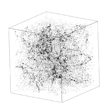
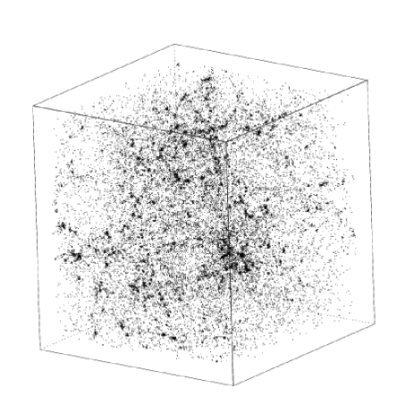
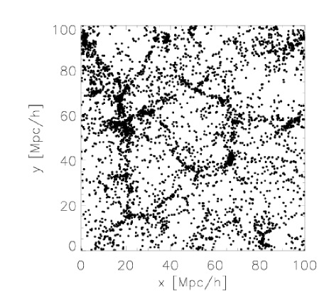
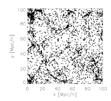
Abbildung 1: Upper panel: Three-dimensional representation of the original simulated OCDM data set (left) and one representation of a surrogate data set (right). The cube length amounts to 100 Mpc/h. Lower panel: Two-dimensional slice of the original (left) and surrogate (right) data set. All points of a slice of 10 Mpc/h in the middle of the cube (45 Mpc/h $<$ z $<$ 55 Mpc/h) are shown.

Before we show the results of our investigations we want to give an outlook concerning the techniques of constrained randomisation: The algorithm described above makes explicit use of the (inverse) Fourier transformation for evenly binned data sets thus limiting the applicability of the method. In our case, where we do have evenly binned data and where we want the surrogates only to have the same power spectrum and the same amplitudes as the original in configuration space, the method is well suited. This might not always be the case. There exist more general approached for the constrained randomisation of data sets (Schreiber 1998 and Schreiber & Schmitz 2000), which rely on the well-known technique of simulated annealing (Metropolis et al. 1953 and Kirkpatrick et al. 1983). In this formalism the constraints are imposed as a cost function which is constructed to have a global minimum when the constraints are exactly fulfilled. With this more flexible but very CPU-time consuming approach arbitrary constraints can be implemented - at least in principle. Thus a systematic analysis of the different statistical measures and their sensitivity to certain constraints in the data becomes possible. Such analysis is beyond the scope of this work, but in future work we will focus on implementing more sophisticated constraints (e.g. higher-order correlations, phase entropy etc.) in the surrogate data sets in order to systematically assess statistical measures used in large scale structure analysis.

5 Results

With the method described in the previous section we generated a set of 20 three-dimensional surrogate data sets from the original OCDM data. In Fig. 1 the three-dimensional point distributions as well as a 2-dimensional slice for the OCDM data and one surrogate realisation are displayed. Looking at the point distributions one does not see very pronounced morphological differences between the original and surrogate data set. One can clearly detect some salient features (e.g. clusters) in both point distributions. If surrogates are generated applying only a simple phase randomisation without taking care of the amplitude distribution (see e.g. the example in Chiang 2001) one obtains a more or less featureless image. Therefore we can conclude that the additional constraint of preserving the amplitude distribution in configuration space is responsible for the existence of morphological features in the point distribution of the surrogate data set. Nevertheless, a thorough eye-inspection of the original and surrogate data set might give the impression that the two point distributions have slightly different topological features. Clusters can be found in the surrogate data set as well as in the original data whereas the fine filament structures as well as the voids are not so pronounced in the surrogates.

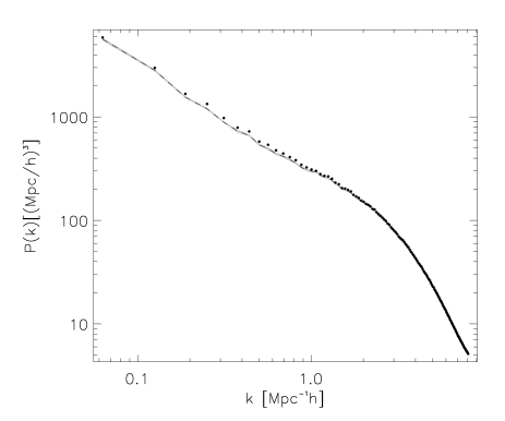
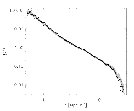
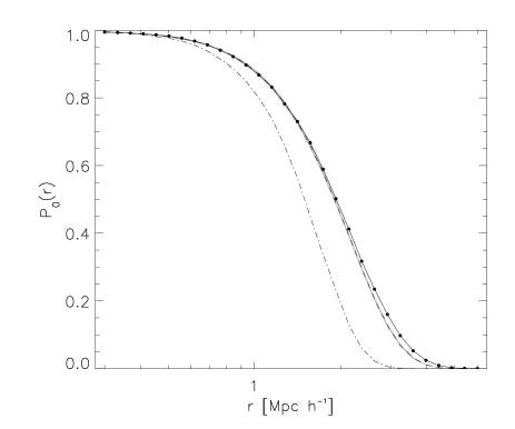
Abbildung 2: Power spectrum (upper row), 2-point correlation function (middle row) and void probability function (lower row) for the original and surrogate data sets. In the left column the respective measured quantities ($P(k)$, $\xi(r)$ and $P_{0}(r)$) for the original (filled circles) and five surrogate (other symbols) data sets are shown. In the right column the measured values of the original data sets are compared with the 1 $\sigma$ error region as derived from 20 realisations of the surrogate data. The dash-dotted line in the diagram for the void probability function indicates the graph for $P_{0}(r)$ in the poissonian case.

The quantitative analysis of the data starts with the calculation of the power spectrum. In Fig. 2 (upper panel) the power spectra of the original and surrogate data sets are shown. They are - as required - (almost) equivalent. For each wave number $k$ the power $P(k)$ for the original data set lies within or only sightly above the $1\sigma$- error region as derived from the power spectra of the 20 surrogates. Likewise the original data and surrogates have the same 2-point correlation function as can be seen in Fig. 2 (middle panel). Only for very low values for $r$ the 2-point correlation function $\xi(r)$ for the original data is outside the mv phases$1\sigma$- error region. At these small distances pixelisation effects become important (pixel size: $0.4$ Mpc/h) so that these deviations from the expected values are understood. The void probability function $P_{0}(r)$ for the data sets is shown in Fig. 2 (lower panel). It can be seen that for higher values of $r$ ($r\approx 1.5$ Mpc/h) the VPF for the surrogates is shifted towards the pure poissonian case and therefore yields slightly lower values than for the original data which are significantly above the $1\sigma$- error area in this region. Hence a discrimination between the original data and surrogates using this measure seems possible. The more poissonian-like behaviour of the surrogate VPF indicates that the higher order correlations in the data are affected by generating the surrogates, making them more randomly distributed. However, the VPF for the surrogates still differs significantly from the pure random case and lies much closer to the VPF of the original data than of the poisson case.

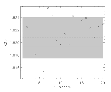
Abbildung 3: Mean phase entropy $<S>=(S_{x}+S_{y}+S_{z})/3$ for the surrogate data (crosses) and the original data (solid line). The gray region indicates the 1 $\sigma$ deviation around the mean (dashed line) as derived from the 20 realisations of the surrogates.

In order to analyse how the Fourier phases are influenced by randomising the original data set we calculated the mean phase entropy $<S>$ for all data sets. The results are displayed in Fig. 3. One can see that for both the original and surrogate data $<S>$ is significantly lower than $\ln{2\pi}\approx 1.838$ which is a clear indication that the phases are not completely uncorrelated but at least partially coupled. Both classes of data are therefore nongaussian. However, in our sample the original data set can not be told apart from the surrogates using the phase entropy. $<S>$ for the OCDM data lies clearly within the $1\sigma$- error region close to the mean of $<S>$ for the surrogates. Thus the phase entropy is a good scalar measure for testing for non-gaussianity but it is obviously not so well suited to discriminate between different non-gaussian point distributions. It may be necessary to define more subtle measures in order to extract the information about the morphology of the structures contained in the correlations of the Fourier phases more efficiently.

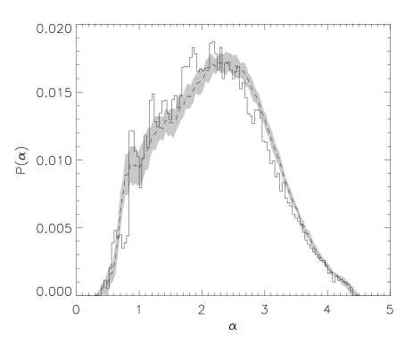
is

Abbildung 4: Probability density of the scaling indices $P(\alpha)$ (r = 4 Mpc/h) for the original and surrogate data sets. Left: $P(\alpha)$ for the original (filled circles) and five surrogate (other symbols) data. Right: $P(\alpha)$ for the original data (black histogram) compared with the 1 $\sigma$ error region (gray area) as derived from 20 realisations of the surrogate data.

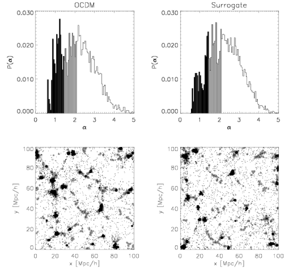
Abbildung 5: Probability density $P(\alpha)$ (upper row) and slices (lower row) for the original and one surrogate data set. Points with $\alpha<1.45$ are merked in black, points having $1.45<\alpha<2.1$ are marked in gray.

The probability distribution $P(\alpha)$ of the weighted scaling indices $\alpha$ for the original data and surrogates is shown in Fig. 4. From the comparison between the mean distribution for the surrogates with its $1\sigma$-error and the $P(\alpha)$-spectrum for the original data as displayed in Fig. 4, one can derive several important results. For a wide range of $\alpha$-vaues the probability distribution $P(\alpha)$ for the OCDM data is significantly outside the $1\sigma$- error region of the surrogates. A clear distinction between the surrogates and the original data is made possible using weighted scaling indices. Thus the weighted scaling indices and their probability distribution $P(\alpha)$ have the highest discriminative power of all statistical measures discussed in this study, making this measure a very promising new candidate for a refined analysis of the large scale structure. Furthermore, a more detailed analysis of the $P(\alpha)$ spectra reveals valuable information about the morphological differences between the original and surrogate data sets. For the surrogates the peak in the $P(\alpha)$ distribution for the OCDM model at $\alpha\approx 0.9$ vanishes, indicating that the percentage of points belonging to highly overdense cluster-like regions diminishes. The location of the maximum of the distribution is shifted from $\alpha\approx 2.0$ for the OCDM data to $\alpha\approx 2.6$ for the surrogates while the height of the peak is retained. These differences of the $P(\alpha)$ distribution are interpreted as a loss of wall-like and filament-like structures in the surrogates with a correspondingly higher percentage of randomly distributed points, which yields higher values for $P(\alpha)$ in the range $2.8<\alpha<3.5$. In order to visualize the loss of cluster-like and filament-like structural elements in the surrogates we extracted all points in slices of the thickness 10 Mpc/h (45 Mpc/h $<$ z $<$ 55 Mpc/h) for the original data one surrogate data set. For these points the $P(\alpha)$-spectrum is determined (see Fig. 5). We now make use of the possibility offered by the scaling index method to extract specific structural elements from the point distribution by selecting the respective regions in the $P(\alpha)$ distribution. For this purpose all points of the slice with $\alpha<1.45$ are marked in black while points having $1.45<\alpha<2.1$ are marked in gray. The differences between the original and surrogate data now become obvious (see Fig. 5). The marked cluster-like (black) and filament-like (gray) points are close together and well connected in the OCDM data, clearly assigning the respective structural elements (clusters or filaments) to which the points belong to, whereas for the surrogate data the selected points are more randomly distributed over the plane and only a smaller percentage of the selected points can clearly be assigned to certain structural elements.

6 Conclusions

We adapted and used the method of surrogate data to analyse three-dimensional point distributions. It could be shown that with the help of the method of iteratively refined surrogates it is possible to generate data sets which have the same power spectrum and amplitude distribution in configuration space but differ significantly with respect to their topological structure. The existence of these topological differences points to nonlinear processes in the early evolution of the universe and is likely to be important cosmologically. Hence nonlinear measures need to be developed to quantify them - after which the consequences for the different models have to be discussed. Amongst the standard measures the void probability function gave relatively small differences between the original and the surrogate data sets, while the 2-point correlation function and power spectrum were the same (by construction).
These results show that linear global measures like the 2-point correlation function and power spectrum are only of limited usefulness for the characterisation of the morphological content of given point distribution and that their discriminative power is, therefore, also limited. This is mainly due to the fact that these second order statistical measures are ’blind’ to the distributions of Fourier phases, which are responsible for the fine details of cosmic structures. We further analysed the distribution of the phases by calculating the phase entropy and found that the surrogates cannot be told apart from the original data set using this measures. Therefore, a more sophisticated analysis of the obviously inherent correlation in the distribution of the phases is required.
We showed that the development of nonlinear morphological descriptors, which are based on the analysis of the local scaling behaviour of the mass distribution, can offer new possibilities to refine our statistical methods so that previously ignored subtle but important features can be both detected and quantitatively characterised. Using such a measure (weighted scaling indices) a clear distinction based on the different topological features between surrogates and the original data set is possible. In the context of evaluating different statistical measures used in the analysis of large scale structure the method of constrained randomisation represents a vital tool with which the quality of the newly developed measures can be tested systematically. Thus a better quantitative characterisation of the spatial patterns in the galaxy distribution becomes possible, improving the interpretation and our outstanding of the large scale structure in the universe.

- [1] Bardeen J.M., Bond J.R., Kaiser N., Szalay A.S., 1986, ApJ, 304, 15
- [2] Bharadwaj S. et al., 2000, ApJ, 528, 21
- [3] Borgani S., 1995, Phys. Rep., 251, 1
- [4] Chiang L.-Y., Coles P., 2000, MNRAS, 311, 809
- [5] Chiang L.-Y., 2001, MNRAS, 325, 405
- [6] Couchman H.M.P., 1999, J. Comp. App. Math., 109, 373
- [7] Coles P., Chiang L.-Y., 2000, Nat., 406, 376
- [8] Colless M. et al., 2001, MNRAS, 328, 1039
- [9] Eke V.R., Cole S., Frenk C.S., 1996, MNRAS, 282, 263
- [10] Fry J.N., Peebles P., 1978, ApJ, 221, 19
- [11] Ghigna S. et al., 1994, ApJ, 437, L71
- [12] Groth E.J., Peebles P., 1977, ApJ, 217, 385
- [13] Hamilton A.J.S., 1993, ApJ, 406, L47
- [14] Hoyle F., Vogeley M., Gott J.R., 2002, ApJ, 570, 44
- [15] Jain A., Farrokhnia F., 1991, Pat. Rec., 24, 1167
- [16] Jamitzky F. et al., 2001, Ultramicrosc., 241
- [17] Julesz B., 1981, Nat., 290, 91
- [18] Julesz B., 1991, Rev. Mod. Phys., 63, 735
- [19] Kerscher M. et al., MNRAS, 284, 73
- [20] Kirkparick K., Gelatt C.D., Vecchi M.P., 1983, Sci., 220, 671
- [21] Mataresse S., Verde L., Heavens A.F., 1997, 290, 651
- [22] Mecke K., Buchert T., Wagner H., 1994, A & A, 288, 697
- [23] Meiskin A., Szapudi I., Szalay A., 1992, ApJ, 394, 87
- [24] Metropolis N., Rosenbluth A., Rosenbluth M., Teller A., Teller E., 1953, J. Chem. Phys., 21, 1097
- [25] Norberg P. et al., 2001, MNRAS, 328, 64
- [26] Paladin G., Vulpiani A., 1987, Phys. Rep., 156, 147
- [27] Pan J., Coles P., 2000, MNRAS, 315, L51
- [28] Peebles P., 1980, The Large Scale Structure of the Universe, Princeton Univ. Press
- [29] Polygiannakis J., Moussas X., 1995, Sol. Phys., 158, 159
- [30] Räth C., Morfill G., 1997, J. Opt. Soc. Am. A, 14, 3208
- [31] Sagi D., Julesz, B., 1985, Sci., 228, 1217
- [32] Seljak U., Zaldamiaga M., 1996, ApJ, 469, 437
- [33] Schreiber T., Schmitz A., 1996, Phys. Rev. Lett., 77, 635
- [34] Schreiber T., Schmitz A., 1997, Phys Rev. E., 55, 5443
- [35] Schreiber T., Schmitz A., 2000, Physica D, 142, 346
- [36] Schreiber T., Phys. Rev. Lett., 1998, 80, 2105
- [37] Schuecker P. et al., A & A, 368, 86
- [38] Scoccimarro R., Feldman H., Fry J., Frieman J., 2001, ApJ, 546, 652
- [39] Sugiyama N., 1995, ApJS, 100, 281
- [40] Szalay A.S. et al., 2001, astro-ph/0107419
- [41] Szapudi I., Postman M., Lauer T., Oegerle W., 2001, ApJ, 548, 114
- [42] Szapudi I. et al., 2002, ApJ, 570, 75
- [43] Tegmark M., Hamilton A., Yongshong X., 2001, astro-ph/0111575
- [44] TheilerJ. et al., 1992, Physica D, 58, 77
- [45] Tuceryan M., Jain A., 1993, in Chen C., Pau L., Wang P.,eds., Handbook of Pattern Recognition and Computer Vision, World Scientific Publishing, 235
- [46] Verde L. et al., 1998, MNRAS, 300, 747
- [47] Vogeley M., Szalay A., 1996, ApJ, 465, 34
- [48] Weinberg D., Gott J.R., Melott A., 1987, ApJ, 321, 2
- [49] White S., 1979, MNRAS, 186, 145
- [50] York D., et al., 2000, AJ, 120, 1579