Cosmological parameters from lensed supernovae

We investigate the possibility of measuring the Hubble constant, the fractional energy density components and the equation of state parameter of the “dark energy” using lensed multiple images of high-redshift supernovae. With future instruments, such as the SNAP and NGST satellites, it will become possible to observe several hundred lensed core-collapse supernovae with multiple images. Accurate measurements of the image separation, flux-ratio, time-delay and lensing foreground galaxy will provide complementary information to the cosmological tests based on, e.g., the magnitude-redshift relation of Type Ia supernovae, especially with regards to the Hubble parameter that could be measured with a statistical uncertainty at the one percent level. Assuming a flat universe, the statistical uncertainty on the mass density is found to be $\sigma^{\rm stat}_{\Omega_{\rm M}}\raise 1.29167pt\hbox{$<$}\kern-7.5pt{\lower 2.79857pt\hbox{$\sim$}}0.05$. However, systematic effects from the uncertainty of the lens modeling are likely to dominate. E.g., if the lensing galaxies are extremely compact but are (erroneously) modeled as singular isothermal spheres, the mass density is biased by $\sigma^{\rm syst}_{\Omega_{\rm M}}\sim 0.1$.

We argue that wide-field near-IR instruments such as the one proposed for the SNAP mission are critical for collecting large statistics of lensed supernovae.

1 Introduction

Gravitational lensing of high-$z$ objects has been used in the past as a tool for deriving cosmological parameters with mixed success. While the fraction of quasars with multiple images and the distribution of image separations may be used to probe the vacuum energy density, $\Omega_{\Lambda}$ (Turner 1990; Schneider et al. 1992), the method suffers from severe systematic uncertainties related to the lens modeling and the results are as of yet inconclusive (Fukugita et al. 1992; Maoz & Rix 1993; Kochaneck 1996; Park & Gott 1997; Chiba & Yoshii 1999). On the other hand, the method proposed by Refsdal (1964, 1966) using time delay measurements of multiple imaged quasars to constrain $H_{0}$ has provided results that are in good agreement with independent techniques, (see e.g. Koopmans & Fassnacht 1999; Brown 2000). Thus, distances derived from geometrical measurements of lensed high-redshift sources may be a viable way to gain further knowledge of cosmological parameters although there are still unresolved issues concerning the modeling of the lenses. E.g. in a recent paper (Kochaneck 2002), five gravitational lens systems are analyzed and it is suggested that, unless the dark matter distributions in the lensing galaxies are rather compact, the derived value of $H_{0}$ is too low in comparison with the local measurements.

In this note we investigate how to use multiply imaged high-redshift supernovae (SNe) to constrain the Hubble parameter, the mass and dark energy density of the universe, $\Omega_{\rm M}$ and $\Omega_{X}$, as well as the equation of state parameter, $w_{0}={p_{X}\over\rho_{X}}$, which we assume is constant for $z\raise 1.29167pt\hbox{$<$}\kern-7.5pt{\lower 2.79857pt\hbox{$\sim$}}5$. SNe are well suited for this technique because of the expected high rate at high-redshifts and most importantly because of their well known lightcurves. In particular, the (rest-frame) optical lightcurves of core-collapse (CC) SNe show fast rise-times, typically about 1 week long. Thus, the time difference between images can be measured to better than one day’s precision.

Another possibility is the use of the UV shock-breakout. As has been seen in SN 1987A and modeled in Ensman & Burrows (1992) the shock breakout can serve as a time stamp with a precision of just minutes. The entire UV flash occurs over a period of minutes to several hours in the rest-frame of the SN depending on the nature of the progenitor.

Wide field optical and NIR deep surveys, such as the planned SNAP satellite (Perlmutter et al. 2001), have the potential to discover $\sim 10^{6}$ CC SNe. While these SNe are sometimes regarded as a “background” for the primary cosmology program based on Type Ia SNe, we argue that lensed SNe of any kind may also provide useful information on cosmological parameters.

In Holz (2001) the number of multiply imaged CC SNe up to $z<2$ were estimated by simply scaling the Type Ia rate by a factor of 5. In this work we extend the considered redshift up to $z=5$ using a SN rate calculation derived from the star formation history. Further, we take into account the NIR wide field instrumentation in the current design of the SNAP satellite.

Using simple toy-models, we investigate the accuracy of the strong lensing technique to improve our knowledge of cosmological parameters. Our observables are the source redshift, the redshift of the lensing galaxy, the image-separation, $\Delta\theta$, the time-delay, $\Delta t$, and the flux-ratio, $r$. We derive the relation of our observables and cosmological parameters for different matter distributions in order to investigate the sensitivity to the choice of lens model. We speculate, that if the measurement is done using a very large sample of lensed systems, useful bounds on the cosmological parameters can be found in spite of large uncertainties in the lens model.

We have used the SNOC Monte-Carlo simulation package (Goobar et al. 2002b) to estimate the rate and measurable quantities of multiple image SNe, e.g. the distribution of time-delays, image-separations and flux-ratios. We also simulate extinction by dust both in the host galaxy of the SN and in the foreground lensing galaxy.

While about half of the known lensed systems exhibit more images (see e.g. Keeton et al. 1998), this work is limited to spherically symmetric lensing systems producing only two or ring-like images. Systems with more lensed images are potentially very interesting as they provide more measurables which can be used to constrain the lens model.

2 Modeling of galaxy halos

In this work, we confine our study to a very simple class of spherically symmetric lens models with projected, two-dimensional lens potential (Schneider et al. 1992)

$$\psi(r)=kr^{\alpha},$$ (1)

where $\alpha\leq 1$ to assure that we get multiple images and that the surface density falls at large radii. The two limiting cases of this class of models are the Singular Isothermal Sphere (SIS) where $\alpha=1$ and the point-mass for which $\alpha=0$ and $k\alpha=1$. A drawback with this choice of single-slope models is that we need steep halo models in order to produce multiple images. A slightly more general treatment would include double slope models like the isothermal sphere with a core (ISC) or the NFW density profile (Navarro et al. 1997). Also, since many multiple image systems have more than two images, the ellipticity of the lensing galaxy should be included in the model. That is, since we assume a very limited class of lens models, we underestimate the systematic effects from the lens modeling. However, we also use a very limited set of observables. In four-image systems, we will have ten observables to use in the fit (four image positions, three flux-ratios and three time-delays) in comparison to the three observables used in this study. Still, there is no doubt that we underestimate the errors in the lensing potential while restricting our study to lens potentials of the form given by Eq. (1). As a first step, we compare results for the two extreme cases of point-masses and SIS density profiles.

2.1 Point-masses

A light ray which passes by a point-mass $M$ at a minimum distance $\xi$, is deflected by the “Einstein angle”

$$\hat{\alpha}=\frac{4M}{\xi}=\frac{2R_{S}}{\xi},$$ (2)

where $R_{S}=2M$ is the Schwarzschild radius. Using a characteristic length $\xi_{0}$ in the lens plane given by

$$\xi_{0}=\sqrt{2R_{S}\frac{D_{d}D_{ds}}{D_{s}}}=\beta_{0}D_{d},$$ (3)

$$\beta_{0}=\sqrt{2R_{S}\frac{D_{ds}}{D_{d}D_{s}}},$$ (4)

where $D_{ds},D_{d}$ and $D_{s}$ are angular diameter distances between deflector and source, deflector and observer, and source and observer respectively. The lens equation in dimensionless form is

$$y=x-1/x,$$ (5)

which has two solutions,

$$x_{1,2}=\frac{1}{2}\left(y\pm\sqrt{y^{2}+4}\right),$$ (6)

i.e., one image on each side of the lens. The image separation is given by

$$\Delta\theta=\beta_{0}\sqrt{y^{2}+4}.$$ (7)

The magnification is given by

$$\mu=\left(1-\frac{1}{x^{4}}\right)^{-1},$$ (8)

which can be combined with Eq. 6 to give

$$\mu_{1,2}=\pm\frac{1}{4}\left[\frac{y}{\sqrt{y^{2}+4}}+\frac{\sqrt{y^{2}+4}}{y}\pm 2\right].$$ (9)

The ratio $r$ of the absolute values of the magnifications (flux-ratio) for the two images produced by a point-mass lens is given by,

$$r=\left|\frac{\mu_{1}}{\mu_{2}}\right|=\left[\frac{\sqrt{y^{2}+4}+y}{\sqrt{y^{2}+4}-y}\right]^{2},$$ (10)

and

$$y=r^{1/4}-r^{-1/4}.$$ (11)

Thus, we can write the image separation in terms of the flux-ratio as

$$\Delta\theta=\beta_{0}(r^{1/4}+r^{-1/4}).$$ (12)

The time delay between images is in the general case given by

$$\Delta t(\@vec{y})=\xi_{0}^{2}\frac{D_{s}}{D_{d}D_{ds}}(1+z_{d})\left[\phi(\@vec{x}^{(1)},\@vec{y})-\phi(\@vec{x}^{(2)},\@vec{y})\right],$$ (13)

where $\phi(\@vec{x},\@vec{y})$ denotes the so called Fermat potential. In the case of a point-mass lens we have

$$\Delta t=2R_{S}(1+z_{d})\tau(y),$$ (14)

where

$$\tau(y)=\frac{1}{2}y\sqrt{y^{2}+4}+\ln\frac{\sqrt{y^{2}+4}+y}{\sqrt{y^{2}+4}-y}.$$ (15)

We can now express $R_{S}$ and $y$ in our observables to get

$$\Delta t=\frac{\Delta\theta^{2}}{2}\frac{D_{d}D_{s}}{D_{ds}}(1+z_{d})\frac{\sqrt{r}-1/\sqrt{r}+\ln{r}}{\sqrt{r}+1/\sqrt{r}+2}.$$ (16)

2.2 Singular isothermal sphere (SIS)

The density profile for the SIS halo, which is frequently used in gravitational lensing analysis, is given by

$$\rho_{{\rm SIS}}(r)=\frac{v^{2}}{2\pi}\frac{1}{r^{2}}.$$ (17)

Here, $v$, the only free parameter of the model, is the line-of-sight velocity dispersion. The simplicity of the SIS density profile allows analytical solutions for the many quantities related to gravitational lensing (Turner et al. 1984). The deflection angle is computed to be

$$\hat{\alpha}(\xi)=4\pi\left(\frac{v}{c}\right)^{2}\frac{|\xi|}{\xi}=:\alpha_{0}\frac{|\xi|}{\xi},$$ (18)

where $\alpha_{0}$ is defined as the magnitude of the deflection. That is, the magnitude of the deflection angle is independent of the impact parameter. Choosing

$$\xi_{0}=4\pi\left(\frac{v}{c}\right)^{2}\frac{D_{d}D_{ds}}{D_{s}},$$ (19)

the lens equation can be written

$$y=x-\frac{x}{|x|}.$$ (20)

Considering $y>0$, there are two images for any $y<1$; at $x=y+1$ and $x=y-1$, i.e., on opposite sides of the lens center. The image separation is given by

$$\Delta\theta=2\alpha_{0}\frac{D_{ds}}{D_{s}},$$ (21)

and the magnification for an image at $x$ is

$$\mu=\frac{|x|}{|x|-1}.$$ (22)

From Eq. (22) we see that the ratio of the absolute values of magnifications of the images is

$$r=\frac{1+y}{1-y}.$$ (23)

The time delay for the two images is

$$\Delta t=\left[4\pi\left(\frac{v}{c}\right)^{2}\right]^{2}\frac{D_{d}D_{ds}}{D_{s}}(1+z_{d})2y,$$ (24)

which can be expressed in terms of our observables as

$$\Delta t=\frac{\Delta\theta^{2}}{2}\frac{D_{d}D_{s}}{D_{ds}}(1+z_{d})\frac{r-1}{r+1}.$$ (25)

We see that only the $r$-dependent part differs between the point and the SIS case. It is reassuring to see that they only differ by at most 6% up to a flux ratio of four. Thus, the derived value of the cosmological parameters are only weakly sensitive to the choice of point or SIS model.

3 Monte-Carlo simulations

Since we in principle only are able to follow infinitesimal light-beams in SNOC, we have to use some approximations when trying to get information on multiple image systems. The main approximation is that we assume that in cases of strong lensing, the effects from one close encounter is dominant, i.e., the one-lens approximation. With this simplification, we can use the information from the magnification to derive quantities for systems with finite separations. In order to do this, we need to be able to derive analytical relations between the magnification and the image-separation and so forth. Here we show how this is done for the case of SIS lenses.

First, we concentrate on primary images. Studying Eqs. (20) and (22), we see that multiple imaging occurs whenever $\mu_{1}>2$ and that the magnification of the second image is given by

$$|\mu_{2}|=\mu_{1}-2.$$ (26)

Using Eq. (21) and the fact that $y=1/(\mu_{1}-1)$, we can write the time-delay for a SIS lens as

$$\Delta t=\left[4\pi\left(\frac{v}{c}\right)^{2}\right]^{2}\frac{D_{d}D_{ds}}{D_{s}}(1+z_{d})\frac{2}{\mu_{1}-1}.$$ (27)

Therefore, in order to compute the quantities of interest, we need to pick a lens redshift and velocity dispersion from some reasonable distributions for every case where $\mu_{1}>2$. The distributions will in general be functions of the cosmology, the mass distribution of the lenses and the source redshift. The differential probability for multiple imaging is in the general case given by

$$dP\propto\sigma(z_{d},z_{s})\frac{dn}{dM}dM(1+z_{d})^{3}dV,$$ (28)

where $\sigma(z_{d},z_{s})$ is the cross-section for multiple imaging and $n$ is the comoving number density of lenses. For SIS lenses, the cross-section is given by

$$\sigma(z_{d},z_{s})\propto\left(\frac{v}{c}\right)^{4}D_{ds}^{2}.$$ (29)

Since $dV\propto D_{d}^{2}\frac{dt}{dz_{d}}dz_{d}$ and $n$ is independent of the lens redshift we can use

$$dP(z_{d})\propto D_{ds}^{2}D_{d}^{2}(1+z_{d})^{3}\frac{dt}{dz_{d}},$$ (30)

as our probability distribution for $z_{d}$. The probability distribution for $v$ is given by

$$dP(v)\propto\frac{dn}{dM}\frac{dM}{dv}\left(\frac{v}{c}\right)^{4}dv.$$ (31)

Following Bergström et al. (2000), we derive a galaxy mass distribution, $dn/dM$, by combining the Schechter luminosity function (Peebles 1993, Eq. 5.129),

$$dn = \phi(y)dy,$$

$$\phi(y) = \phi_{*}y^{\alpha}e^{-y},$$ (32)

$$y = \frac{L}{L_{*}},$$

with the mass-to-luminosity ratio (Peebles 1993, Eq. 3.39),

$$\frac{M}{M_{*}}=y^{1/(1-\beta)}.$$ (33)

Using Eq. (32), we find that

$$\frac{dn}{dM} \propto y^{\delta}e^{-y},$$ (34)

$$\delta = \alpha-\frac{\beta}{1-\beta}.$$ (35)

Combining the Faber-Jackson relation

$$\frac{v}{v_{*}}=y^{\gamma},$$ (36)

where $y$ is defined in Eq. (32), with the mass-to-luminosity ratio, Eq. (33), we can relate the velocity dispersion to mass by

$$\frac{v}{v_{*}}=\frac{M}{M_{*}}^{\gamma(1-\beta)}.$$ (37)

In this paper we use $v_{*}=220$ km s^-1, $\alpha=-1.07$, $\beta=0.2$ and $\gamma=0.25$. The mass normalization is calculated assuming that the entire mass of the resides in galaxy halos (Bergström et al. 2000).

A higher value of $v_{*}$ would result in a larger number of wide separation lenses since the cross-section for multiple imaging scales as $\sigma\propto v^{4}$ [see Eq. (29)] and the image separation as $\Delta\theta\propto v^{2}$ [Eq. (21)]. Varying the galaxy mass distribution will also have an effect on the characteristics of the lensed events. However, since the mass and velocity dispersion are not variables in the fitting of cosmological parameters (see Sect. 5), any changes in these distributions will only have a marginal effect on the results obtained in this paper.

4 Characteristics of lensed SN events

We have simulated $1.1\cdot 10^{6}$ CC SNe in the redshift range $0\leq z\leq 5$ using a SIS model for the galaxy density profiles. The redshift dependence of the SN rates, the relative fraction among the various types of CC SNe (Ib/c, IIL, IIn, IIP, 87a-like), peak magnitudes and intrinsic dispersion were simulated following the prescriptions in Dahlén & Fransson (1999) and Dahlén & Goobar (2002). Using SN rate predictions derived from the star formation history (Chugai et al. 1999; Sullivan et al. 2000), our simulated sample corresponds approximately to the predicted number of CC SN explosions ($z\leq 5$) in a period of 3-years in a 20 square degree field, i.e., $\sim 5.1$ SNe year^-1arcmin^-2. In the simulations we have assumed a flat cosmology with $\Omega_{\rm M}$ = 0.3 and $\Omega_{\Lambda}$ = 0.7, and a Hubble constant $H_{0}=65$ km s^-1Mpc^-1. We view these rates on the conservatively low side given the recent work by Lanzetta et al. (2002) who finds that the SFR plausibly increases monotonically with redshift through the highest redshifts observed.

Out of the $1.1\cdot 10^{6}$ simulated CC SNe, 2613 were multiply lensed. Fig. 1 shows the number of detectable SNe as a function of the peak-brightness threshold in I and J-bands. The threshold refers to the faintest of the two images.

Figure 1: Number of multiple image SNe in the simulated sample vs magnitude threshold for the faintest image in I and J-band.

In the following analysis, we consider two possible data samples (all magnitudes are in the Vega system):

• case A: only SNe with an I-band peak magnitude of the faintest image of m${}_{\rm I}\leq 28.5$

• case B: SNe where either the I-band peak brightness or the J-band brightness falls below 28.5 mag (i.e. m_I or m${}_{\rm J}\leq$ 28.5)

Thus, only 211 (case A) and 366 (case B) lensed CC SNe were considered for cosmology fits. Additional potential SNe discovered in other bands are thus not considered in this study. For an instrument like SNAP (wavelength sensitivity 0.4-1.7 $\mu$m), revisiting each field in at least one optical or NIR band every 6 (or less) hours, we expect a very high detection efficiency. E.g., assuming that the SNe were discovered 0.5 magnitudes below peak brightness, SNAP would be able to make a 5$\sigma$ detection every four days in each of three (or more) filters: I, Z , J and possibly others.

In the simulations we have considered the possibility that one or both images suffer extinction. We assumed differential extinction properties as in Cardelli et al. (1989), with $R_{V}=3.1$ and a mean-free path of 1 kpc for V-band photons in the host and lensing galaxy. Details of the simulation procedure can be found in Goobar et al. (2002a, b).

In Figs. 2–5, we show the distribution of observables for the multiple-image SNe; source redshifts, image flux-ratios, image separations and time-delay between the images. The dashed lines show the subset of the data fulfilling case A SNe while the dotted curves correspond to case B.

The salient features of the events are: images of the same source with average redshift $z_{s}\approx 2$ and the lensing galaxy typically at $z_{d}\sim z_{s}/2$. The SN images are separated by $\sim$ 0.5 arcseconds and a few weeks apart. With the imposed minimal brightness criteria, the images differ typically by less than one astronomical magnitude. Clearly, a very clean signature to search for, especially with space observations free of atmospheric blurring.

Figure 2: Redshift distribution of lensed SNe up to $z=5$, solid line. The dotted line shows SNe for which the SN system satisfies the case B criteria. The dashed lines shows case A. A SIS lens profile was used. The lensing galaxy is typically at a redshift $\sim z_{s}/2$

Figure 3: Flux-ratio of SN images. The dotted line shows SNe for which the SN system satisfies the case B criteria. The dashed line shows case A. A SIS lens profile was used.

Figure 4: Image separation in arcseconds. The dotted line shows SNe for which the SN system satisfies the case B criteria. The dashed line shows case A. A SIS lens profile was used.

Figure 5: Time delay between the SN images in days. The dotted line shows SNe for which the SN system satisfies the case B criteria. The dashed line shows case A. A SIS lens profile was used.

5 Fitting cosmological parameters

Next, we estimate the target statistical uncertainty of a 3 year mission studying a 20 square degree patch of the sky down to 28.5 peak I-band (and J-band) magnitudes. We perform a maximal likelihood analysis of the multiply lensed systems with $h,\Omega_{\rm M}$ and $\Omega_{\Lambda}$ as free parameters where $h$ is the dimensionless Hubble parameter defined by $H_{0}=h\cdot$100 km s^-1Mpc^-1. With $\@vec{\phi}=(h,\Omega_{\rm M},\Omega_{\Lambda})$ and $f(r)$ being the $r$-dependent factors in Eqs. (16) and (25) for point mass lenses and SIS respectively we define the “experimental” ($R_{\rm exp}$) and cosmology dependent (${\cal R}$) quantities:

$$R_{\rm exp}=2{\Delta t\over{\Delta\theta}^{2}}\left({1+z_{d}\over f(r)}\right)^{-1}{\rm and}$$

$${\cal R}(\@vec{\phi})={D_{d}\cdot D_{s}\over D_{ds}}.$$

The maximum likelihood analysis performed over the simulated SNe with index $i=$1..N assumes Gaussian probability density functions for the observables,

$${\cal L}=\prod_{i}{1\over\sqrt{2\pi\sigma}}e^{-(R_{\rm exp}^{i}-{\cal R(\@vec{\phi}}))^{2}/2\sigma^{2}},$$ (38)

where the standard deviation $\sigma$ contains the propagated uncertainties of the (independent) observables $\@vec{x}=(\Delta t,\Delta\theta,r,z_{d})$:

$$\sigma^{2}=\sum_{j=1}^{4}{\left({\partial R_{\rm exp}\over\partial x_{j}}\sigma_{x_{j}}\right)^{2}}.$$ (39)

For simplicity, we have assumed that all SNe are measured with the same precision.

While we will consider more pessimistic scenarios later, in this section we assume that the uncertainties $\sigma_{x_{j}}$ of the four observables are:

$$\left\{\begin{array}[]{lcl}\sigma_{\Delta t}&=&0.05{\rm\ days}\\ \sigma_{\Delta\theta}&=&0.01^{\prime\prime}\\ \sigma_{r}&=&0.1\\ \sigma_{z_{d}}&=&0.001\end{array}\right.$$ (44)

The outstanding precision in the time delay between the SN images is consistent with the estimates of the accuracy expected for SNIa lightcurves studied with simulations by the SNAP collaboration.

The image separation uncertainty corresponds to 0.1 pixel of the proposed SNAP instrument. This estimate could even improve considering that all of the SN images along the lightcurve can be co-added to get $\raise 1.29167pt\hbox{$>$}\kern-7.5pt{\lower 2.79857pt\hbox{$\sim$}}40\sigma$ signals on the individually lensed SNe. E.g. in Anderson & King (2000) it is stated that with HST/WFPC one could reach 0.02 pixel precision on reasonable bright stars.

In estimating $\sigma_{r}$ we have assumed that the differential extinction of the lensed SNe will not largely exceed what has been measured for a set of 23 gravitational lens galaxies in Falco et al. (1999). The median extinction for those systems ($z_{d}\raise 1.29167pt\hbox{$<$}\kern-7.5pt{\lower 2.79857pt\hbox{$\sim$}}1$) was found to be $E(B-V)\sim 0.05$ mag.

5.1 The $\Omega_{\rm M}-\Omega_{\Lambda}$ plane

While ${\cal R}\propto h^{-1}$, it varies only weakly with $\Omega_{\rm M}$ and $\Omega_{X}$. This can be appreciated from the projected 68 % confidence level (CL) region from a 3-parameter fit ($\Omega_{\rm M},\Omega_{\Lambda},h$) to the simulated data-set B in Fig. 6. From now on we concentrate on the case B sample. The areas covered by the contour regions of case A scale approximately as $\sqrt{N_{B}/N_{A}}$. It should be noted that the shape and inclination of CL region is very different from what is found from the magnitude-redshift test (Goobar & Perlmutter 1995). We also show in dark the constraints in the $\Omega_{\Lambda}-\Omega_{\rm M}$ plane if $h$ is known (exactly). While little information can be gained from $\Omega_{\rm M}$ or $\Omega_{\Lambda}$ independently, the figures indicate that there is only a very limited range in $\Omega_{\rm M}$ and $\Omega_{\Lambda}$ for which the CL region is consistent with a flat universe, $\Omega_{\rm M}+\Omega_{\Lambda}=1$. Thus, from now on, we concentrate on the cases where the geometry is assumed to be known from, e.g., CMB anisotropy measurements.

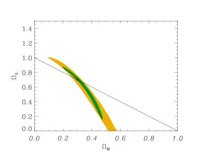
Figure 6: 68 % CL region in the $\Omega_{\rm M}-\Omega_{\Lambda}$ projection of a three parameter fit $(\Omega_{\rm M},\Omega_{\Lambda},h)$. The 366 two-image events fulfilling criteria B. The dark (green) region shows the 68 % CL region that would result if $h$ would be exactly known from independent measurements. The line shows $\Omega_{\rm M}+\Omega_{\Lambda}=1$, i.e. a flat universe. The diamond shows the value that was used in the simulation.

5.2 The $\Omega_{\rm M}-h$ plane

With large statistics, such as the case in our simulations, it is feasible to constrain the possible values of $\Omega_{\rm M}$ if a flat universe is assumed. Fig. 7 shows the 68 % CL-region of the $\Omega_{\rm M}-h$ plane for case B. The dark shaded region shows the systematic effect introduced by fitting the SIS simulated data with the assumption of point mass lenses. The fit in the light shaded region (solid curve) of Fig. 7 yields $h=0.65^{+0.006}_{-0.003}$; $\Omega_{\rm M}=0.30^{+0.04}_{-0.05}$. The uncertainties are 68 % CL for a two parameter fit, i.e., 1.51 $\sigma$. Introducing the bias due to the wrong lens model, we found the fitted central values to be $h=0.69$ and $\Omega_{\rm M}=0.19$. To further test potential bias in the cosmological parameters from systematic uncertainties in the lens model we have tested adding an ad-hoc offset with a different dependence on the image ratio:

$$R_{\rm exp}^{b}=R_{\rm exp}(1+\epsilon r^{2}),$$ (45)

where $\epsilon=\pm 0.001$ and $\pm 0.005$ and the considered uncertainties in the fit are as in Eq. 44. The effect is shown as dotted and dashed curves in Fig. 7. Note, however, that in these examples we are assuming that all lensing galaxies are wrongly modeled. Thus, in that sense, it should be a conservative estimate of the systematic uncertainties.

It is interesting to note that if the Hubble parameter and the energy densities are known to good accuracy from other cosmological tests, it should be possible to put very useful constraints on the average lens properties.

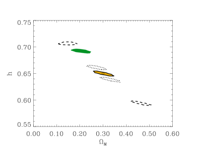
Figure 7: The light (yellow) shaded region bounded by the solid line shows 68 % CL region of $\Omega_{\rm M}-h$ fit from 366 two-image events where the peak brightness of the faintest image fulfills criteria B. A flat universe was assumed. The dark (green) shaded region shows the bias introduced if the fit is done (erroneously) assuming a point-mass lens model. The dotted and dashed curves show the effect of a systematic error in the lens model, according to Eq. 45

5.3 The $\Omega_{\rm M}-w_{0}$ and $h-w_{0}$ planes

Next, we investigate the potential of this method in setting limits in the $\Omega_{\rm M}-w_{0}$ parameter plane. Fig. 8 shows that upper limits on the equation of state parameter of dark energy, $w_{0}<-0.8$ may be derived from the considered data sample. Meaningful limits on the possibility of $w_{0}<-1$ could be derived, especially if an independent estimate of $H_{0}$ is used as a prior in the fit.

Due to the different reshift distributions considered, the shape of the CL-regions differ from what is expected from the Hubble diagram of Type Ia SNe for the SNAP satellite (Goliath et al. 2001). In particular, if the Hubble parameter is further constrained by some independent method, the estimates of $w_{0}$ from the strong lensing data becomes comparable in precision the limits that may be derived from Type Ia SNe, the dashed countour line in Fig. 8. The other 2D projection, the one onto the $w_{0}-h$ plane, is shown in Fig. 9. If the wrong halo model is used in the fitting procedure, i.e., a point-mass halo model instead of SIS, a 5 % bias is introduced in the estimate of $w_{0}$.

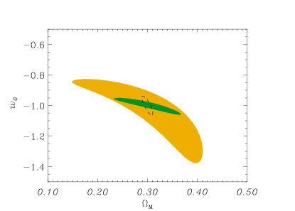
Figure 8: 68 % CL region of $\Omega_{\rm M}-w_{0}$ fit from the 366 events fulfilling criteria B. A flat universe was assumed. The dark (green) region shows the smaller confidence region that would result if $h$ would be exactly known from independent measurements. The dashed line shows the expected statistical uncertainty from a 3 year SNAP data sample of Type Ia SNe.

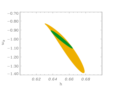
Figure 9: 68 % CL region of $h-w_{0}$ fit from 366 two-image events in case B. A flat universe was assumed. The dark (green) region shows smaller confidence region that would result if $\Omega_{\rm M}$ would be exactly known from independent measurements.

6 Summary and conclusions

Strongly gravitationally lensed SNe could be detected in large numbers in planned wide field, deep, SN search programs, probably on the order of several hundred. In particular, we argue in favor of large NIR imagers in space missions like SNAP.

Lensed SNe are potentially interesting as they provide independent measurements of cosmological parameters, mainly $H_{0}$, but also the energy density fractions and the equation of state of dark energy. The results are independent of, and would therefore complement the Type Ia program. At the faint limits considered in this note, several quasars per square arcminute are expected (Conti et al. 1999). Thus, we expect that an instrument like SNAP would find several hundred multiply imaged QSOs, in addition to the strongly lensed SNe. Thus, the statistical uncertainty could become smaller than what we have considered here.

While the systematic uncertainties remain a source of concern, we show that the simplest spherically symmetric models introduce moderate biases ($\sigma^{\rm syst}_{\Omega_{\rm M}}\raise 1.29167pt\hbox{$<$}\kern-7.5pt{\lower 2.79857pt\hbox{$\sim$}}0.1$) , at least as long as multiple images with similar fluxes are considered.

While projections of different SNe could in principle be interpreted as a lensed SN the two scenarios may be distinguished. The signatures of CC SNe are unique. Crudely, the lightcurves are a product of the progenitor mass, the mass loss during its evolution off the main sequence, the amount of radioactive Ni synthesized during the explosion and the kinetic energy imparted to the ejecta. In addition, the environments the SNe explode in (the density and structure of their local interstellar medium), often play a significant role in what we eventually see of the CC event. These differences have given rise to all the different classifications of these events we currently have; Type IIP, IIL, Ib, Ic, IIn, etc. Given all this diversity it makes it quite easy to distinguish one event from another and to not confuse a lensing event with a coincident CC event along the same line of sight.

In our simulations we find that extinction in the foreground galaxies does not severely affect the detectability of multiple lensed events nor the ability to derive the flux-ratio between the images. Clearly, multi-band observations of the SNe will be important in order to correct for the different amounts of extinction of the images. At the same time, the data could provide important results on the dust properties of the foreground lensing galaxies, similar to the studies done with multiple imaged quasars at $z_{d}\raise 1.29167pt\hbox{$<$}\kern-7.5pt{\lower 2.79857pt\hbox{$\sim$}}1$ (Falco et al. 1999). Unlike quasars, CC events have a very deliberate color evolution along their lightcurves. In general, from the moment of shock-breakout onwards, the atmospheres of CC SNe expand and become cooler and redder. This signature not only helps in the relative timing of these events, but also allows us to measure the differential extinction due to the varying amounts of dust along the lensed paths to the SN quite well. With 3 or more filters one could make a measurement of both the total extinction relative to the bluest event in addition to the ratio of the total to selective extinction due to differences in the dust properties. Furthermore, one could enhance this method by taking a spectrum of the SN (any of the lensed events would do) at a given epoch and through spectrum synthesis derive the true, unextinguished spectral energy distribution of the event [see e.g. (Mitchell et al. 2002; Baron et al. 2002)].

References

- Anderson & King (2000) Anderson, J., & King, I. R. 2000, PASP, 112, 1360
- Baron et al. (2002) Baron, E. et al. 2002, in preparation.
- Bergström et al. (2000) Bergström, L., Goliath, M., Goobar, A., & Mörtsell, E. 2000, A&A, 358, 13
- Brown (2000) Browne, I. W. A. 2000, in ASP Conf. Ser., Gravitational Lensing: Recent Progress and Future Goals, ed. T. G. Brainerd, & C. S. Kochanek (San Francisco: ASP).
- Cardelli et al. (1989) Cardelli, J. A., Clayton, G. C., & Mathis, J. S., 1989, ApJ, 345, 245
- Chiba & Yoshii (1999) Chiba, M., & Yoshii, Y. 1999, ApJ, 510, 42
- Chugai et al. (1999) Chugai, N., Blinnikov, S., & Lundqvist, P., 1999, astro-ph/9901298
- Conti et al. (1999) Conti, A., Kennefick, J. D., Martini, P., & Osmer, P. S., 1999, AJ 117, 645
- Dahlén & Fransson (1999) Dahlén, T., & Fransson, C. 1999, A&A, 350, 349
- Dahlén & Goobar (2002) Dahlén, T., & Goobar, A. 2002, PASP, March issue, in press.
- Ensman & Burrows (1992) Ensman, L., & Burrows, A. 1992, ApJ, 393, 742
- Falco et al. (1999) Falco E. E., Impey, D., Kochanek, C. S., et al.,1999, ApJ, 523, 617
- Fukugita et al. (1992) Fukugita, M., Futamase, T., Kasai, M., & Turner, E. L. 1992, ApJ, 393, 3
- Goliath et al. (2001) Goliath, M., Amanullah, R., Astier, P., Goobar, A., & Pain, R., 2001, A&A 380, 6
- Goobar & Perlmutter (1995) Goobar, A., & Perlmutter, S. 1995, ApJ, 450, 14
- Goobar et al. (2002a) Goobar, A., Bergström,L., & Mörtsell, E., 2002a, A&A, 384, 1
- Goobar et al. (2002b) Goobar, A., Mörtsell, E., Amanullah, R., Goliath. M., Bergström, L., & Dahlén, T. 2002b, A&A in press, astro-ph/0206409
- Holz (2001) Holz, D., 2001, ApJ, 556, L71
- Keeton et al. (1998) Keeton, C. R., Kochanek, C. S., & Falco, E. E., 1998, ApJ, 509, 561
- Kochaneck (1996) Kochanek, C. S., 1996, ApJ, 466, 638
- Kochaneck (2002) Kochanek, C. S., 2002, Submitted to ApJ, astro-ph/0204043
- Koopmans & Fassnacht (1999) Koopmans, L. V. E., & Fassnacht, C. D. 1999, ApJ, 527, 513
- Lanzetta et al. (2002) Lanzetta, K. M., Yahata, N., Pascarelle, S., Chen, H., & Fernández-Soto, A., 2002, ApJ, 570, 492
- Maoz & Rix (1993) Maoz, D., & Rix, H.-W. 1993, ApJ, 416, 425
- Mitchell et al. (2002) Mitchell, R. C, Baron, E., Branch, D., et al., 2002, ApJ in press, astro-ph/0204012
- Navarro et al. (1997) Navarro J. F., Frenk C. S., & White S. D. M., 1997, ApJ, 490, 493
- Park & Gott (1997) Park, M.-G., & Gott, J. R., III. 1997, ApJ, 489, 476
- Peebles (1993) Peebles, P. J. E. 1993, Principles of physical cosmology (Princeton University Press, Princeton)
- Perlmutter et al. (2001) Perlmutter, S., et al. (The SNAP collaboration), 2001, AAS, 199, 1160
- Refsdal (1964) Refsdal, S. 1964, MNRAS, 128, 307
- Refsdal (1966) Refsdal, S. 1966, MNRAS, 132, 101
- Schneider et al. (1992) Schneider, P., Ehlers, J., & Falco, E. E. 1992, Gravitational Lenses (Springer-Verlag, Berlin)
- Sullivan et al. (2000) Sullivan, M., Ellis, R., Nugent, P, Smail, I., & Madau, P., 2000, MNRAS, 319, 549
- Turner et al. (1984) Turner, E. L., Ostriker, J. P., & Gott, J. R. 1984, ApJ, 284, 1
- Turner (1990) Turner, E. L., 1990, ApJ, 365, 43