Statistical characteristics of observed Ly-$\alpha$ forest
and the shape of initial power spectrum

Abstract

Properties of about 4 500 observed Ly-$\alpha$ absorbers are investigated using the model of formation and evolution of DM structure elements based on the modified Zel’dovich theory. This model is generally consistent with simulations of absorbers formation, describes reasonably well the Large Scale Structure observed in the galaxy distribution at small redshifts and emphasizes the generic similarity of the LSS and absorbers.

The simple physical model of absorbers asserts that they are composed of DM and gaseous matter. It allows us to estimate the column density and overdensity of DM and gaseous components and the entropy of the gas trapped within the DM potential wells. The parameters of DM component are found to be consistent with theoretical expectations for the Gaussian initial perturbations with the WDM–like power spectrum. The basic physical factors responsible for the absorbers evolution are discussed.

The analysis of redshift distribution of absorbers confirms the self consistency of the adopted physical model, Gaussianity of the initial perturbations and allows to estimate the shape of the initial power spectrum at small scales what in turn restricts the mass of the dominant fraction of DM particles to $M_{DM}\geq~{}1.5-5$ keV. Our results indicate a possible redshift variations of intensity of the UV background by about a factor of 2 – 3 at redshifts $z\sim$ 2 – 3.

1 Introduction

One of the most perspective methods to study the processes responsible for the formation and evolution of the structure of the Universe is the analysis of properties of absorbers observed in spectra of the farthest quasars. The great potential of such investigations was discussed already in Oort (1981, 1984) just after Sargent et al. (1980) established the intergalactic nature of the Ly-$\alpha$ forest. The available Keck and VLT high resolution observations of the forest provide a reasonable database and allow to apply statistical methods for such investigations.

The essential progress achieved recently through numerous high resolution simulations of absorbers formation and evolution confirms that this process is closely connected with the initial power spectrum of perturbations. These results allow us to consider the properties of absorbers in the context of nonlinear theory of gravitational instability (Zel’dovich 1970; Shandarin & Zel’dovich 1988) and to apply the statistical description of structure formation and evolution (Demiański & Doroshkevich 1999, 2002; hereafter DD99 & DD02) to the Ly-$\alpha$ forest.

This approach is based on the modified Zel’dovich approximation and describes the formation and evolution of DM structure elements for the CDM and WDM initial power spectra without any smoothing or filtering procedures. It outlines the structure evolution as a random formation and merging of Zel’dovich pancakes, their transverse expansion and/or compression and transformation into high density clouds and filaments. Later on, the hierarchical merging of pancakes, filaments and clouds forms rich galaxy walls observed at small redshifts. Main stages of this evolution are driven by the initial power spectrum.

At small redshifts the main results of the statistical approach are found to be consistent with characteristics of the observed and simulated Large Scale Structure (Demiański et al. 2000; Doroshkevich, Tucker & Allam 2002). Here we use this approach for the analysis and interpretation of the absorbers observed at large redshifts. We show that the basic observed characteristics of Ly-$\alpha$ forest are also successfully described in the framework of this theoretical model.

The application of this approach to Ly-$\alpha$ forest was already discussed in Demiański, Doroshkevich & Turchaninov (2001 a,b, hereafter Paper I & Paper II). Here we improve this analysis by using a richer and more refined sample of $\sim$ 4500 observed absorbers and a more refined model of absorbers. Our approach uses more traditional methods of investigation of properties of discrete absorbers rather then associating them with a continuous non-linear line-of-sight density field (see, e.g., Weinberg et al. 1998; McDonald et al. 2000; Croft et al. 2001; Croft et al. 2002). It allows to reach more clarity in the description of formation and evolution of absorbers and to reveal its strong link with the initial power spectrum. It allows also to separate several subpopulations of absorbers and to discuss their evolutionary history.

The composition and spatial distribution of observed absorbers is complicated and at low redshifts a significant number of stronger Ly-$\alpha$ lines and metal systems is associated with galaxies (Bergeron et al. 1992; Lanzetta et al. 1995; Tytler 1995; Le Brune et al. 1996). However as was recently shown by Penton, Stock and Shull (2002), even at small redshifts some absorbers are associated with galaxy filaments while others are found within galaxy voids. These results suggest that the population of weaker absorbers dominating at higher redshifts can be associated with weaker structure elements formed by the non luminous baryonic and DM components in extended low density regions. In turn, the relatively homogeneous spatial distribution of absorbers implies a more homogeneous spatial distribution of both DM and baryonic components as compared with the observed distribution of the luminous matter.

For the truncated Zel’dovich theory (Coles, Melot &  Shandarin 1993; Bond & Wadsley 1997), some statistical characteristics of absorbers were already discussed in Gnedin & Hui (1996); Hui, Gnedin & Zhang (1997); and Hui & Rutledge (1999). In particular, in these papers possible fits for the number density of absorbers with a threshold hydrogen column density, $N_{HI}$, or with a threshold Doppler parameter, $b$, were proposed. However, because of the complex evolution of absorbers, these functions depend upon both the initial power spectrum and several random factors discussed below (Secs. 2.3, 4.3). So, the application and interpretation of these fits are limited.

Here we use a statistical approach (DD02) based on the modified Zel’dovich theory which describes both linear and nonlinear evolution of the DM structure. For the CDM–like power spectrum and Gaussian initial perturbations it gives the expected mean 1D number density and the probability distribution function of DM pancakes. Both functions depend only on the cosmological model and moments of the initial power spectrum. Comparison of these functions with absorbers distributions confirms the self consistency of adopted physical model and Gaussianity of the initial density perturbations, allows to estimate the spectral moments and to restrict the mass of dominant DM particles. These results complement the investigations of the linear power spectrum (see, e.g., Croft, Weinberg, Katz & Hernquist 1998; Gnedin & Hamilton 2002; Zaldarriaga, Scoccimorro & Hui 2002; Croft et al. 2002).

However, this theory does not describe the process of relaxation of compressed matter, the disruption of structure elements due to the gravitational instability of DM pancakes and the distribution of neutral hydrogen across DM pancakes. Now we have only limited information about properties of the background gas and UV radiation (Scott et al. 2000; Schaye et al. 2000; McDonald & Miralda–Escude 2001; McDonald et al. 2000, 2001; Theuns et al. 2002a, b). Therefore, in this paper some numerical factors remain undetermined. They could be more precisely determined by special investigations of simulated and observed absorbers.

This analysis should be supplemented by application of the discussed here approach to simulations which take simultaneously into account the impact of many important factors and provide unified picture of the process of absorbers formation and evolution (see, e.g., Weinberg et al. 1998; Zhang et al. 1998; Davé et al. 1999; Theuns et al. 1999). But so far such simulations can be performed only in small boxes what restricts their representativity, introduces artificial cutoffs in the power spectrum and complicates the quantitative description of structure evolution (see more detailed discussion in Hui & Gnedin 1997 and Paper II). The semianalitic models (see, e.g., Bi & Davidsen 1997; Choudhury, Padmanabhan & Srianand 2001; Choudhury, Srianand, & Padmanabhan 2001; Viel et al. 2002) show other perspective approach to study the structure evolution at high redshifts. Perhaps, some results obtained below can be also useful for this purpose.

Comparison of results obtained in Paper I and Paper II and in this paper demonstrates that the quality and representativity of the sample of observed absorbers are very important for the reconstruction of processes of absorbers formation and evolution. In this paper we use the sample of $\sim$ 4500 absorbers at 1.7 $\leq~{}z\leq$ 4 compiled from 18 high resolution spectra. However, the redshift distribution of absorbers is inhomogeneous what increases errors and generates some uncertainties. In particular, the statistics of absorbers at $z\geq$ 3.5 is very poor. Because of the preliminary character of our investigation we estimate the precision of only the most important parameters.

Further progress can be achieved with richer samples covering the range of redshifts at least up to $z\sim$ 4.5–5. The observational evidence of the reheating of the Universe at $z\approx$ 6 (Djorgovski et al 2001; Fan et al. 2001) makes it important to perform a complex investigation of the early period of structure evolution at redshifts $z\sim$ 4–6.

This paper is organized as follows. The theoretical model of the structure evolution is discussed in Sec. 2. In Sec. 3 the observational databases used in our analysis are presented. The results of statistical analysis are given in Secs. 4–6. Discussion and conclusion can be found in Sec. 7 .

2 Model of absorbers formation and evolution

The main observational characteristics of absorption lines are the redshift, $z_{abs}$, the column density of neutral hydrogen, $N_{HI}$, and the Doppler parameter, $b$, while the theoretical description of structure formation and evolution is dealing with the mean linear number density of absorbers, $n_{abs}(z)$, temperature, overdensity and entropy of DM and gaseous components, and with the ionization degree of hydrogen. To connect these theoretical and observed parameters a physical model of absorbers formation and evolution is required.

Many such models were proposed and discussed during the last twenty years (see references in Rauch 1998, and in Paper I and Paper II). However, to describe the properties of the new wider and refined sample of observed absorbers it is necessary to develop a more detailed physical model of absorbers as well. Our model includes some ideas discussed already in earlier publications.

2.1 Physical model of absorbers.

In this paper we assume that:

1. The DM distribution forms an interconnected structure of sheets (Zel’dovich pancakes) and filaments, their main parameters are approximately described by the Zel’dovich theory of gravitational instability applied to the CDM or WDM initial power spectrum (DD99; DD02). The majority of DM pancakes are partly relaxed, long-lived, and their properties vary due to the successive merging and expansion and/or compression in the transverse directions.

2. Gas is trapped in the gravitational potential wells formed by the DM distribution. The gas temperature and the observed Doppler parameter, $b$, trace the depth of the DM potential wells.

3. For a given temperature, the gas density within the wells is determined by the gas entropy created during the previous evolution. The gas entropy is changing, mainly, due to shock heating in the course of merging of pancakes, bulk heating produced by the UV background and local sources and due to radiative cooling.

4. The gas is ionized by the UV background and for the majority of absorbers ionization equilibrium is assumed.

5. The observed properties of absorbers are changing because of merging, transversal compression and/or expansion and disruption of DM pancakes. The bulk heating and radiative cooling leads to slow drift of the entropy and density of the trapped gas. Random variations of the intensity and spectrum of the UV background enhance random scatter of the observed absorbers properties.

6. In this simple model we identify the velocity dispersion of DM component compressed within pancakes with the temperature of hydrogen and the Doppler parameter $b$ of absorbers. We consider the possible macroscopic motions within pancakes as subsonic and assume that they cannot essentially distort the measured Doppler parameter.

As compared with the model discussed in Paper II, here we take into account more accurately the evolution of pancakes after their formation.

The formation of DM pancakes as an inevitable first step of evolution of small perturbations was firmly established both by theoretical considerations (Zel’dovich 1970; Shandarin & Zel’dovich 1989) and numerical simulations (Shandarin et al. 1995). Both theoretical analysis and simulations show the successive transformation of sheet-like elements into filamentary-like ones and, at the same time, the merging of both sheet-like and filamentary elements into richer walls. Such continuous transformation of structure goes on all the time. These processes imply the existence of a complicated time-dependent internal structure of high density elements and, in particular, the unavoidable arbitrariness in discrimination of such elements into filaments and sheets.

Our approximate consideration cannot be applied to objects for which the gravitational potential and the gas temperature along the line of sight strongly depends on the matter distribution across this line. In this paper we use the term ’pancake’ to denote structure elements with relatively small gradient of properties along the line of sight. With such a criterion, the anisotropic halo of filaments and clouds can be also considered as ’pancake-like’.

The subpopulation of weaker absorbers also contains ”artificial” caustics (McGill 1990) and absorbers identified with slowly expanding underdense regions (Bi & Davidsen 1997; Zhang et al. 1998; Davé et al. 1999). Such absorbers produce a short lived noise, which is stronger at higher redshifts $z\geq$ 3. Fortunately, fraction of such absorbers does not exceed 10–15% of the observed sample and they cannot significantly distort our final estimates.

In this paper we consider the spatially flat $\Lambda$CDM model of the Universe with the Hubble parameter and mean density given by:

$$H^{2}(z)=H_{0}^{2}\Omega_{m}(1+z)^{3}[1+\Omega_{\Lambda}/\Omega_{m}(1+z)^{-3}]\,,$$ (1)

$$\langle\rho_{m}(z)\rangle={3H_{0}^{2}\over 8\pi G}\Omega_{m}(1+z)^{3},\quad H_{0}=100h\,{\rm km/s/Mpc}\,.$$

Here $\Omega_{m}=0.3\,\&\,\Omega_{\Lambda}=0.7$ are dimensionless matter density and the cosmological term, and $h=$ 0.65 is the dimensionless Hubble constant.

2.2 Properties of the homogeneously distributed hydrogen

Properties of the compressed gas can be suitably related to the parameters of homogeneously distributed gas, which were discussed in many papers (see, e.g., Ikeuchi & Ostriker 1986; Hui  & Gnedin 1997; Scott et al. 2000; McDonald et al. 2001; Theuns et al. 2002a, b). Thus, the baryonic density and temperature can be taken as

$$\langle n_{b}(z)\rangle=2.4\cdot 10^{-7}{\rm cm}^{-3}(1+z)^{3}(\Omega_{b}h^{2}/0.02)\,,$$ (2)

$$T_{bg}\approx 1.6\cdot 10^{4}K\theta_{bg}^{2}(z),\quad b_{bg}=\sqrt{2k_{B}T_{bg}\over m_{H}}\approx 16\theta_{bg}{\rm km/s}\,.$$

Here $\Omega_{b}$ is the dimensionless mean density of baryons, $T_{bg}\,\&\,b_{bg}$ are the temperature and Doppler parameter of the gas, $\theta_{bg}^{4}(z)\sim 1+z$ describes a slow decrease of temperature with redshift for low density cosmological models, $k_{B}\,\&\,m_{H}$ are the Boltzmann’s constant and the mass of the hydrogen atom.

Under the assumption of ionization equilibrium of the gas,

$$\alpha_{r}n_{b}^{2}\approx n_{H}\Gamma_{\gamma},\quad\alpha_{r}(T)\approx 4\cdot 10^{-13}\left({10^{4}K\over T}\right)^{3/4}{{\rm cm}^{3}\over{\rm s}}\,,$$ (3)

where $\alpha_{r}(T)$ is the recombination coefficient (Black, 1981) and $\Gamma_{\gamma}$ characterizes the rate of ionization by the UV background, the fraction of neutral hydrogen is

$$x_{bg}=n_{H}/n_{b}=\langle n_{b}(z)\rangle~{}\alpha_{r}(T_{bg})\Gamma_{\gamma}^{-1}=x_{0}(1+z)^{3},$$ (4)

$$x_{0}\approx{6.7\cdot 10^{-8}\over\Gamma_{12}}{\Omega_{b}h^{2}\over 0.02}\left({16km/s\over b_{bg}(z)}\right)^{3/2},\quad\Gamma_{\gamma}=10^{-12}s^{-1}\Gamma_{12}\,,$$

For the standard power law spectrum of radiation we get

$$J(\nu)=J_{21}\cdot 10^{-21}\left({\nu_{H}\over\nu}\right)^{\alpha_{\gamma}}erg~{}s^{-1}cm^{-2}sr^{-1}Hz^{-1}\,,$$

$$\Gamma_{12}=12.6J_{21}(3+\alpha_{\gamma})^{-1}\,.$$

The gas entropy can be characterized by the function

$$F_{bg}={T_{bg}\over\langle n_{b}\rangle^{2/3}}={36{\rm keV\cdot cm}^{2}\over(1+z)^{2}}\left({0.02\over\Omega_{b}h^{2}}\right)^{2/3}\left({b_{bg}(z)\over 16km/s}\right)^{2}\,.$$ (5)

2.3 Parameters of absorbers

In this section we introduce the main relations between theoretical and observed characteristics of pancakes based on the physical model discussed in Sec. 2.1. The most important characteristics of DM pancakes are presented (without proofs) as a basis for further analysis. For more details see DD99 and DD02.

2.3.1 Characteristics of DM component

The fundamental characteristic of DM pancakes is the dimensional, $\mu$, or the dimensionless, $q$, Lagrangian thickness (the dimensionless DM column density) :

$$\mu\approx{\langle\rho_{m}(z)\rangle l_{v}q\over(1+z)}={3H_{0}^{2}\over 8\pi G}l_{v}\Omega_{m}(1+z)^{2}q\,,$$ (6)

$$l_{v}\approx{6.6\over h\Omega_{m}}h^{-1}{\rm Mpc}=33.8h^{-1}{\rm Mpc}{0.3\over\Omega_{m}}{0.65\over h}\,,$$

where $l_{v}$ is the coherent length of initial velocity field (DD99; DD02). The Lagrangian thickness of a pancake, $l_{v}q$, is defined as the unperturbed distance at redshift $z=0$ between DM particles bounding the pancake. The actual thickness of a pancake is

$$\Delta r=\mu\rho_{m}^{-1}=l_{v}q(1+z)^{-1}\delta^{-1},\quad\delta=\rho_{m}/\langle\rho_{m}(z)\rangle\,.$$ (7)

Here $\delta$ is the mean overdensity of a pancake above the background density.

Comparing the pancake surface density, $\mu(z)$, with the distance between neighboring absorbers,

$$D_{sep}={c\Delta z\over H(z)}=5.5\cdot 10^{3}{\Delta z\over(1+z)^{3/2}}\sqrt{0.3\over\Omega_{m}}h^{-1}{\rm Mpc}\,,$$ (8)

we can also estimate the fraction of matter accumulated by absorbers as

$$f_{abs}\simeq{\mu(1+z)\over\langle\rho_{m}\rangle D_{sep}}\approx 6.2\cdot 10^{-3}q{(1+z)^{3/2}\over\Delta z}\sqrt{0.13\over\Omega_{m}h^{2}}\,.$$ (9)

The fraction of clustered matter characterized by $\langle f_{abs}(z)\rangle$ can be compared with theoretical expectations (see Sec. 4.4).

For Gaussian initial perturbations, the expected probability distribution function for the DM column density is

$$N_{q}dq\approx{2\over\sqrt{\pi}}e^{-\xi}~{}{{\rm erf}(\sqrt{\xi})\over\sqrt{\xi}}\left({q^{2}\over q^{2}+q_{0}^{2}}\right)^{3/4}d\xi,\quad\xi={q\over 8\tau^{2}}\,,$$ (10)

$$\langle\xi\rangle\approx{1\over 2}+{1\over\pi}\approx 0.82,\quad\langle\xi^{2}\rangle\approx{3\over 4}+{2\over\pi},\quad\langle\xi^{3}\rangle\approx{3\over 16}+{11\over 2\pi}\,,$$

(DD02), where the parameter $q_{0}\ll$ 1 characterizes the coherent length of the initial density field (see Sec. 7.5) and the dimensionless ’time’ $\tau(z)$ describes the evolution of perturbations in the Zel’dovich theory. For $\Lambda$CDM model (1) and $z\geq 2$ we have

$$\tau(z)\approx\tau_{0}\left({1+1.2\Omega_{m}\over 2.2\Omega_{m}}\right)^{1/3}{1\over 1+z}\approx{1.27\tau_{0}\over 1+z}\,,$$ (11)

and for the amplitude of perturbations (Doroshkevich, Tucker & Allam 2002)

$$\tau_{0}\approx(0.27\pm 0.04)\sqrt{\Omega_{m}h\over 0.2},\quad\xi\approx 1.06q(1+z)^{2}{0.2\over\Omega_{m}h}\,.$$ (12)

Strictly speaking, relations (6) and (10) are valid for pancakes formed and observed at the same redshift $z_{obs}=z_{f}$ and after pancake formation the transverse expansion and compression changes its DM column density. However, as was shown in DD02, these processes do not change the statistical characteristics of pancakes observed at redshift $z_{obs}\leq z_{f}$. This means that statistically we can consider each pancake as created at the observed redshift. More details are given in DD99 and DD02.

For the DM dominated cosmological model the observed Doppler parameter is also closely linked with properties of the DM pancakes. Thus, in Paper II the $b$–parameter was identified with the infall velocity of matter into pancakes:

$$b\approx v_{inf}=u_{0}(z)\sqrt{\xi^{2}+2\xi}\,,$$ (13)

$$u_{0}(z)\approx 2.3l_{v}H_{0}\tau^{2}\sqrt{1+z}\approx{310km/s\over(1+z)^{3/2}}\sqrt{0.13\over\Omega_{m}h^{2}}\,.$$

This assumption is valid also some time after formation of the pancake but later on the pancake relaxation, compression and/or expansion in transverse directions change the $b$–parameter.

As is seen from (13), for $\langle\xi\rangle$ independent from redshift (10), a systematic variation of the mean Doppler parameter with redshift could be expected. The problem was left open in Paper II (due to limited observational data set) but now, with the more representative sample of absorbers, we see surprisingly weak redshift variations of the mean observed Doppler parameter (Sec. 4.1). This means that only small fraction of observed absorbers is ’young’ and is described by (13), whereas ’older’ relaxed and gravitationally confined absorbers dominate this sample. The simple model of relaxed absorbers was already considered in Paper II. Here we substantially improve it.

As is well known, for an equilibrium slab of DM the depth of potential well is

$$\Delta\Phi\approx{\pi G\mu^{2}\over\langle\rho(z)\rangle\delta}\Theta_{q}^{2}\Theta_{\Phi}\,,$$ (14)

where random factors $\Theta_{\Phi}\,\&\,\Theta_{q}$ characterizes the nonhomogeneity of DM distribution across the slab and the evaporation of matter in the course of its relaxation.

Analysis of numerical simulations (Demiański et al. 2000) indicates that the relaxed distribution of DM component can be approximately described by the politropic equation of state with the power index $\gamma\approx$ 2 . In this case, we can expect that

$$\Theta_{\Phi}={2\gamma\over\sqrt{\pi}(\gamma-1)}{\Gamma(1.5-1/\gamma)\over\Gamma(1-1/\gamma)}={4\over\pi}\,.$$

where $\Gamma(y)$ is Euler function. The actual distribution of DM component across a slab and the value of $\Theta_{\Phi}$ depend upon the relaxation process which is essentially accelerated due to the pancake disruption into the system of high density clouds and filaments. This means that the factor $\Theta_{\Phi}$ randomly vary from absorber to absorber.

At each pancake merging $\sim$ 10 – 15% of matter is evaporated due to the violent relaxation. This means that $\Theta_{q}\sim$ 1 for absorbers formed from the homogeneously distributed matter and $\Theta_{q}$ decreases for rich absorbers formed due to several successive mergings.

The Doppler parameter is defined by the depth of potential well and for the isentropic gas with $p_{gas}\propto\rho_{gas}^{5/3}$ trapped within the well, we get

$$b^{2}\approx{4\over 5}\Delta\Phi\approx{4\over 5}{\pi G\mu^{2}\over\langle\rho(z)\rangle\delta}\Theta_{q}^{2}\Theta_{\Phi}=\delta_{0}b_{bg}^{2}{q^{2}\over\delta}(1+z)\,,$$ (15)

$$\delta_{0}={3\over 10}\left({H_{0}l_{v}\over b_{bg}}\right)^{2}\Omega_{m}\Theta_{\Phi}\Theta_{q}^{2}\approx 4\cdot 10^{3}\Theta_{\delta}\,,$$

$$\Theta_{\delta}=\left({0.13\over\Omega_{m}h^{2}}\right)\left({16km/s\over b_{bg}(z)}\right)^{2}\Theta_{\Phi}\Theta_{q}^{2}\,.$$

Variations of the gas entropy across an absorber increase the random variations of $\Theta_{\delta}$ and $b$.

2.3.2 Characteristics of gaseous component

The observed column density of neutral hydrogen can be written as an integral over a pancake along the line of sight

$$N_{HI}=\int dx~{}\rho_{b}x_{H}=2\langle x_{H}\rangle{\langle n_{b}(z)\rangle l_{v}q\over 1+z}{0.5\over cos\theta}\,.$$ (16)

Here $\langle x_{H}\rangle$ is the mean fraction of neutral hydrogen and $cos\theta$ takes into account the random orientation of absorbers and the line of sight ($\langle cos\theta\rangle\approx 0.5)$. We assume also that both DM and gaseous components are compressed together and, so, the column density of baryons and DM component are proportional to each other.

However, the overdensity of the baryonic component, $\delta_{b}=n_{b}/\langle n_{b}\rangle$ is not identical to the overdensity of DM component, $\delta$, (see, e.g., discussion in Matarrese & Mohayaee 2002). Indeed, the gas temperature and the Doppler parameter are mainly determined by the characteristics of DM component (15) but the gas overdensity is smaller than that of DM component due to larger entropy of the gas. Moreover, the bulk heating and cooling change the density and entropy of the gas trapped within the DM potential well. Under the assumption of ionization equilibrium of the gas (3) this process is described by the equation

$${1\over n_{b}}{dn_{b}\over dt}=n_{b}\alpha_{r}(T)[\varepsilon(T)-T_{\gamma}/T],\quad T=T_{bg}b^{2}/b_{bg}^{2}\,,$$ (17)

where the recombination coefficient $\alpha_{r}(T)$ was given in (4), $T_{\gamma}\sim(5-10)\cdot 10^{4}$K characterizes the energy injected at a photoionization and

$$\varepsilon(T)\approx 2T_{4}^{1/4}[1-0.3\ln T_{4}+0.13T_{4}^{1/3}],\quad T_{4}=T/10^{4}K\,,$$

describes the radiative cooling for the bremsstrahlung emission and recombination of hydrogen and helium (Black 1981).

The energy injected at the photoionization, $T_{\gamma}$, depends upon the spectrum of local UV background and it varies randomly with time and space. The gas temperature varies because of the pancake expansion and compression and due to the pancake disruption into a system of high density clouds. As is seen from (17), these processes change the baryonic density of pancakes and we can write

$$\delta_{b}=\kappa_{b}(z)\delta\,.$$ (18)

This means that the factor $\kappa_{b}$ is small for absorbers formed due to adiabatic and weak shock compression because of the large difference between entropies of the background DM and the gas, and $\kappa_{b}\rightarrow$ 1 for richer hot absorbers formed due to strong shock compression when this difference becomes small.

Under the assumption of ionization equilibrium of the gas (3) and neglecting a possible contribution of macroscopic motions to the $b$-parameter ($T\propto b^{2}$), for the fraction of neutral hydrogen and its column density we get:

$$\langle x_{H}\rangle=x_{0}\kappa_{b}(z)\delta\beta^{-3/2}(1+z)^{3}\Theta_{x},\quad\beta=b/b_{bg}\,,$$

$$N_{HI}=N_{0}q\delta\beta^{-3/2}(1+z)^{5},\quad N_{0}=5\cdot 10^{12}cm^{-2}\Theta_{H}\,,$$ (19)

$$\Theta_{H}={\kappa_{b}\Theta_{x}\over\Gamma_{12}}{0.13\over\Omega_{m}h^{2}}{\langle cos\theta\rangle\over cos\theta}\left({\Omega_{b}h^{2}\over 0.02}\right)^{2}\left({16km/s\over b_{bg}(z)}\right)^{3/2}\,,$$

where $\Gamma_{12}$, $b_{bg}$ and $x_{0}$ were defined in (2) and (4) and the factor $\Theta_{x}$ describes the nonhomogeneous distribution of ionized hydrogen along the line of sight.

2.3.3 Absorbers characteristics

Eqs. (15) and (19) link the observed and other physical characteristics of absorbers. For the DM column density, $q$, the average gas entropy, $\Sigma=\ln(F_{s})$, and overdensity, $\delta$, we get:

$$q^{3}={N_{HI}\over N_{0}\delta_{0}}{\beta^{7/2}\over(1+z)^{6}},\quad\delta=\delta_{0}{q^{2}\over\beta^{2}}(1+z)\,,$$ (20)

$$\exp(\Sigma)=F_{s}=\beta^{2}/\delta_{b}^{2/3}=\kappa_{b}^{-2/3}\beta^{2}/\delta^{2/3}\,.$$

Here we use the standard equation of state $T/T_{bg}=\beta^{2}(z)=F_{s}(z)\delta^{2/3}(z)$ .

The precision of these estimates is moderate and the main uncertainties are generated by the unknown cos$\theta$ and parameters $\Theta_{\Phi}$, $\Theta_{q}$, $\Theta_{x}$, $\kappa_{b}$ and $\Gamma_{\gamma}$, which vary – randomly and systematically – from absorber to absorber (estimates of $q$ and $\delta$ are independent from $b_{bg}$). These variations distort parameters defined in (20) as follows:

$$q^{3}\propto{1\over\Theta_{H}\Theta_{\delta}},\quad\delta^{3}\propto{\Theta_{\delta}\over\Theta_{H}^{2}},\quad F_{s}\propto\kappa_{b}^{-2/3}\left({\Theta_{H}^{2}\over\Theta_{\delta}}\right)^{2/9}\,.$$ (21)

Independent estimates of these uncertainties can be obtained from the analysis of the redshift distribution of absorbers (Sec. 6).

However, comparing the average DM column density of pancakes, $\langle q\rangle$, with expectations (10) we can restrict the possible redshift variations of $\langle\Theta_{H}\Theta_{\delta}\rangle$ and estimate the combined uncertainty introduced by unknown factors. As is seen from (20),

$$\xi^{3}\approx(1+z)^{6}~{}q^{2}=\left({N_{HI}\over 2\cdot 10^{16}cm^{-2}}\right)\left({b\over 16km/s}\right)^{7/2}G_{12}\,,$$

$$G_{12}(z)={\Gamma_{12}\over\kappa_{b}\Theta_{x}\Theta_{\Phi}\Theta_{q}^{2}}{cos\theta\over 0.5}\left({\Omega_{m}h^{2}\over 0.13}{\Omega_{b}h^{2}\over 0.02}\right)^{2}\,.$$ (22)

This relation shows that, for statistically homogeneous sample of absorbers with $\langle\xi^{3}\rangle=const.$, $\langle cos\theta\rangle=$ 0.5, we can estimate the redshift variations of $\langle G_{12}(z)\rangle$ as follows:

$$\langle G_{12}(z)\rangle\propto\left\langle{\Gamma_{12}\over\kappa_{b}\Theta_{x}\Theta_{\Phi}\Theta_{q}^{2}}\right\rangle\propto\langle\xi^{3}\rangle/\langle N_{HI}b^{7/2}\rangle\,.$$

Precision of these estimates is limited because of strong random scatter of the product $N_{HI}b^{7/2}$ .

2.3.4 Regular and random variations of absorber characteristics

The most fundamental characteristic of absorbers is their DM column density, $\xi\approx q(1+z)^{2}$. It describes the formation and merging of pancakes, is only weakly sensitive to the action of random factors and defines the regular variations of the Doppler parameter, $b$, overdensity, $\delta$, and entropy, $F_{s}$. These parameters include also a random component which integrates the evolutionary history of each pancake and the action of random factors discussed in the previous subsection. If the structure of a relaxed pancake can be described by the politropic equation of state with the effective power index $\gamma$ then we can discriminate the regular and random variations of $b,\,\delta,\,\&\,F_{s}$ and introduce the reduced characteristics of relaxed absorbers, $\upsilon,\,\Delta\,\&\,S$:

$$\upsilon=\ln[\beta\xi^{(1/\gamma-1)}]\,,$$

$$\Delta=\ln[(1+z)^{3}\delta/\xi^{2/\gamma}]=\ln(\delta_{0})-2\upsilon\,,$$ (23)

$$S=\ln[(1+z)^{-2}F_{s}\xi^{2(5/3-\gamma)/\gamma}]=const.+10\upsilon/3\,.$$

These relations indicate that, in fact, our approximate description use only one random characteristic, namely, $\upsilon$, which is expressed through observed parameters as follows:

$$\upsilon={7-\gamma\over 6\gamma}\ln~{}\beta-{\gamma-1\over 3\gamma}\ln\left({N_{HI}\over N_{0}\delta_{0}}\right)\,.$$ (24)

As is shown in Secs. 4.5.2, the choice of a suitable value of $\gamma$ allows to minimize the correlation between $\xi$ and $\upsilon$. Of course, this reduction is approximate and it can be achieved only statistically for a given sample of absorbers.

2.4 Mean number density of absorbers

Following Paper I we will characterize the 1D mean number density of absorbers by the dimensionless function

$$n_{abs}={c\over H_{0}}\langle l\rangle^{-1}={H(z)\over H_{0}}{dN(z)\over dz}\,.$$ (25)

Here $dN(z)$ is the mean number of absorbers between $z$ and $z+dz$, $\langle l(z)\rangle$ is the mean free path between absorbers at redshift $z$ and $c$ is the speed of light. When absorbers are identified with the Zel’dovich pancakes, this 1D mean number density can be linked with the fundamental characteristics of the cosmological model and moments of the initial power spectrum (DD02 & Sec. 7.5).

As was shown in DD02, for Gaussian initial perturbations and for richer DM pancakes with sizes significantly larger than the coherent length of initial density field, this number density can be approximated by the expression

$$n_{abs}\approx{c\over H_{0}l_{v}}{W_{p}(\xi_{thr})(1+z)^{2}\over\langle q(\xi_{thr})\rangle}\,,$$ (26)

$$\langle q(\xi_{thr})\rangle=4\tau^{2}\left[1+{4\sqrt{\pi\xi_{thr}}\mbox{erf}(\sqrt{\xi_{thr}})+2\exp(-\xi_{thr})\over\pi\exp(\xi_{thr})[1-\mbox{erf}^{2}(\sqrt{\xi_{thr}})]}\right]\,,$$

$$W_{p}(\xi_{thr})\approx 0.5[1-\mbox{erf}(\sqrt{\xi_{thr}})]\,,$$

where $\xi_{thr}(z)=q_{thr}/8\tau^{2}(z)$, $q_{thr}(z)$ is the minimal (threshold) DM column density of pancakes, $W_{p}(\xi_{thr})$ and $\langle q(\xi_{thr})\rangle$ are the fraction of matter and the mean DM column density for pancakes with $q\geq q_{thr}$ and the factor $(1+z)^{2}$ describes the cosmological expansion of pancakes population.

The expression (26) contains only one fitting parameter, $\xi_{thr}$, and it describes quite well the evolution of richer pancakes. However, application of this relation to evolution of weaker pancakes is problematic as for $\xi_{thr}\ll$ 1 we get from (26):

$$n_{abs}\approx 55(1+z)^{4}\,,$$

and this relation does not contain any fitting parameters.

The formation of pancakes with small $q$ is suppressed due to the small scale cutoff in the initial power spectrum. For pancakes with small $q_{thr}$ the redshift variations of the mean number density is described by the expression

$$n_{abs}\approx{c\over H_{0}l_{v}}{\sqrt{3}(1+z)^{2}\over 16\pi\tau(z)\sqrt{q_{0}}}{\mbox{erf}(\sqrt{\xi_{thr}})\over\sqrt{\xi_{thr}}}\exp(-\xi_{thr})\,,$$ (27)

(DD02) where again $\xi_{thr}(z)=q_{thr}(z)/8\tau^{2}$ and the value $q_{0}$ characterizes the coherent length of the initial density field (see Sec. 7.5).

Both expressions, (26) and (27), are derived for the Gaussian initial perturbations. They are valid for DM pancakes formed due to both linear and nonlinear compressions and allow for merging of pancakes. Moreover, as was shown in DD02, if the observed redshift is identified with the redshift of pancake formation then both relations remain the same even when the transverse compression and expansion of pancakes are also taken into account. This means that they partly account for the pancake disruption as well.

The relation (27) describes also the impact of the gaseous pressure on the formation of observed absorbers. In this case, the parameter $q_{0}$ must be calculated with the power spectrum corrected for the Jeans damping of small scale perturbations in the baryonic component (see Sec. 7.5).

2.5 Observational restrictions

The completeness of the observed samples of absorbers is restricted by the condition $N_{HI}\geq N_{thr}\approx 10^{12}cm^{-2}$ what in turn distorts the characteristics of observed absorbers and makes it difficult to compare them with the theoretical expectations discussed in Secs. 2.3 and 2.4 . This means that these expectations should be corrected for the impact of the threshold column density of observed absorbers.

Thus the investigation of spatial distribution of galaxies in the SDSS EDR (Doroshkevich, Tucker & Allam 2002) results in estimates of typical parameters of galaxy walls at small redshifts as

$$\langle q\rangle\approx 0.4,\quad\langle\beta\rangle\approx 20,\quad\langle\delta\rangle\approx 3\,.$$ (28)

With these data the expected column density of neutral hydrogen within the typical wall (16) is

$$N_{HI}\approx 0.02N_{0}\approx 0.1N_{thr}\Theta_{H}\leq N_{thr}\,.$$

This means that even so spectacular object as the ’Greet Wall’ does not manifest itself as absorbers. Rare absorbers with $b\geq$ 100 km/s, $N_{HI}\sim 10^{13}cm^{-2}$ and $\xi\sim$ 1.5 observed at $z\sim$ 1.5 – 4 can be associated with embryos of wall–like elements of the Large Scale Structure of the Universe (see Sec. 5 for more detailed discussion).

For absorbers associated with ’young’ pancakes the Doppler parameter is given by (13) and for the richer ’young’ pancakes with the mean DM column density we get

$$\xi\approx 1,\quad q\approx\langle q\rangle\approx(1+z)^{-2},\quad\beta\approx 35(1+z)^{-3/2}\,,$$

$$\delta\approx 3~{}\Theta_{\delta},\quad N_{HI}\approx 10^{-2}(1+z)^{21/4}N_{0}\Theta_{\delta}\,,$$ (29)

and such pancakes can be seen as absorbers already at redshifts $z\geq$ 1.

For more numerous poorer pancakes with $q\leq\langle q\rangle$ we have

$$\beta\sim 30\sqrt{q}(1+z)^{-1/2},\quad\delta\approx 4q(1+z)^{2}\Theta_{\delta}\,,$$ (30)

$$N_{HI}\approx 2.5\cdot 10^{-2}N_{0}q^{5/4}(1+z)^{31/4}\Theta_{\delta}$$

$$\approx\left({q\over 0.02}\right)^{5/4}\left({1+z\over 2.5}\right)^{31/4}N_{thr}\Theta_{\delta}\Theta_{H}\,,$$

and such pancakes become visible for $z\geq$ 1.5 only.

These rough estimates of expected characteristics of absorbers show that:

1. At redshifts $z\leq$ 1.5 we can observe mainly old pancakes formed at higher redshifts which kept the measurable column density of neutral hydrogen up to small redshifts.

2. The expected number density of observed absorbers rapidly increases at redshifts $z\sim$ 1.5 – 2 when even relatively poor ’young’ pancakes can pass over the observational threshold and become seen as weak absorbers.

This means that our analysis can be applied to absorbers observed at $z\geq$ 1.5 – 2 when the impact of the observational threshold becomes moderate.

2.6 Variations of the UV background

Direct estimates of the intensity of UV background through the proximity effect (Scott et al. 2000) give $\Gamma_{12}\approx 2\pm 1$ at $z\sim$ 2.5 – 3 while McDonald & Miralda-Escude (2001) got $\Gamma_{12}\sim 0.7-0.4$ at the same $z$. Indirect estimates of $\Gamma_{12}$ (Songaila 1998) demonstrate a probable sudden drop of the UV intensity of about 3 times at $z\sim$ 3. This effect can be related to the strong ionization of HeII at these redshifts (Jacobsen et al. 1994; Zeng, Davidsen & Kriss 1998; Theuns at al. 2002a, b).

As is shown in Sec. 6.2, possible redshift variations of $\Gamma_{12}$ are also seen in the redshift distribution of weaker absorbers at $z\approx$ 2.5. These variations can be fitted by the expression

$$\Gamma_{12}={a_{0}+1\over 2}\left[1+{a_{0}-1\over a_{0}+1}{\rm th}\left({z-z_{\gamma}\over 0.16}\right)\right]\,,$$ (31)

where $a_{0}\sim$ 1.5 – 3 and $z_{\gamma}\sim$ 2.5 – 3 characterize the amplitude and the redshift of these variations. These estimates can be distorted due to the limited representativity of our sample and a nonhomogeneous redshift distribution of observed absorbers plotted in Fig. 1 .

However, weak redshift variations of the functions $\langle b\rangle,$ $\langle\lg(N_{HI})\rangle\,\&\,\langle G_{12}\rangle$ (Sec. 4.1) show that the influence of variations of $\Gamma_{12}$ on the properties of absorbers is partly compensated by variations of $\kappa_{b}$, $\Theta_{x}$, $\Theta_{q}\,\&\,\Theta_{\Phi}$ introduced in Secs. 2.3.1 &  2.3.2 . As is found in Sec. 4.2, a reasonable description of the mean absorbers characteristics is achieved when the function $\langle G_{12}\rangle$ (22) is

$$\langle G_{12}\rangle\approx G_{0}(1-0.17z),\quad G_{0}=50\,.$$ (32)

Comparison of this function with estimates of $\Gamma_{12}$ (Scott et al. 2000; McDonald & Miralda-Escude 2001) allows to estimate the unknown factors as

$$\langle\kappa_{b}\Theta_{x}\Theta_{\Phi}\Theta_{q}^{2}\rangle\sim(0.1-0.05)\left({\Omega_{m}h^{2}\over 0.13}{\Omega_{b}h^{2}\over 0.02}\right)^{2}\,.$$

More accurate estimate of these factors can be obtained with numerical simulations.

Table 1: QSO spectra used

	$z_{em}$	$z_{min}$	$z_{max}$	No
				of HI lines
$0000-260^{1}~{}$	4.11	3.4	4.1	431
$0055-259^{2}~{}$	3.66	3.0	3.6	534
$0014+813^{3}~{}$	3.41	2.7	3.2	262
$0956+122^{3}~{}$	3.30	2.6	3.1	256
$0302-003^{3,2}$	3.29	2.6	3.1	356
$0636+680^{3}~{}$	3.17	2.5	3.0	313
$1759+754^{4}~{}$	3.05	2.4	3.0	307
$1946+766^{5}~{}$	3.02	2.4	3.0	461
$1347-246^{2}~{}$	2.63	2.1	2.6	361
$1122-441^{2}~{}$	2.42	1.9	2.4	353
$2217-282^{2}~{}$	2.41	1.9	2.3	262
$2233-606^{6}~{}$	2.24	1.5	2.2	293
$1101-264^{2}~{}$	2.15	1.6	2.1	277
$0515-441^{2}~{}$	1.72	1.5	1.7	76
$2126-158^{7}~{}$	3.26	2.9	3.2	130
$1700+642^{8}~{}$	2.72	2.1	2.7	85
$1225+317^{9}~{}$	2.20	1.7	2.2	159
$1331+170^{10}~{}$	2.10	1.7	2.1	69

1. Lu et al. (1996), 2. unpublished, courtesy of Dr. Kim 3. Hu et al., (1995), 4. Djorgovski et al. (2001) 5. Kirkman & Tytler (1997), 6. Cristiani & D’Odorico (2000), 7. Giallongo et al. (1993), 8. Rodriguez et al. (1995), 9. Khare et al. (1997), 10. Kulkarni et al. (1996).

3 The database.

The present analysis is based on the 18 spectra listed in Table 1. The available Ly-$\alpha$ lines were arranged into three samples. The richest sample, $S_{14}^{12}$, includes 4369 absorbers with $10^{15}cm^{-2}\geq N_{HI}\geq 10^{12}cm^{-2}$ from the first 14 high resolution spectra. It can be partly incomplete. For comparison, we use the most reliable sample $S_{18}^{13}$ which includes 2643 absorbers from all 18 spectra for $10^{13}cm^{-2}\leq N_{HI}\leq 10^{15}cm^{-2}$ . These lines are more easily identified and they are not so sensitive to outer random influences. The sample $W_{14}^{12}$ contains 2126 weaker lines with $N_{HI}\leq 10^{13}cm^{-2}$ from the first 14 QSOs. It is mainly used to characterize possible variations of the UV background. To decrease the scatter of absorbers characteristics we exclude from these samples 45 absorbers with $b\geq$ 90km/s .

As is seen from Fig 1, for all samples the redshift distribution of absorbers is nonhomogeneous and the majority of absorbers are concentrated at 2 $\leq z\leq$ 3 . This means that some of the discussed absorbers characteristics are derived mainly from this range of redshifts. Absorbers at $z\geq~{}3.5$ were identified mainly from the spectrum of QSO 0000-260 (Lu et al. 1996) and here the line statistics is insufficient.

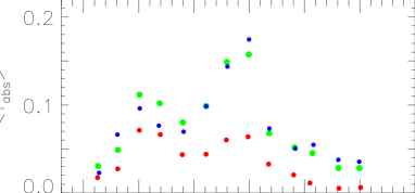
Figure 1: Redshift distribution of the fraction of observed absorbers for samples $W_{14}^{12}$ (red points), $S_{14}^{12}$ (green points) and $S_{18}^{13}$ (blue points).

4 Statistical characteristics of absorbers

In this Section, the functions $q,\xi,\delta~{}\&~{}F_{s}$ are found for the $\Lambda$CDM cosmological model (1) with $b_{bg}=$ 16km/s, $\Omega_{b}h^{2}=$ 0.02 and the function $\langle G_{12}(z)\rangle$ given by (32) with

$$G_{0}=50,\,\Theta_{\delta}=\langle\Theta_{\Phi}\Theta_{q}^{2}\rangle=0.5,\,\Theta_{H}=\left\langle{\kappa_{b}\Theta_{x}\over\Gamma_{12}}\right\rangle=0.1.$$ (33)

Some quantitative results of this Section depend on the completeness and representativity of the samples and the quite arbitrary choice of $\Theta_{\delta}\,\&\,\Theta_{H}$ (33) through the relations (21). As was noted above, for each absorber these factors change in the course of absorbers evolution and, in fact, the accepted values are averaged over the sample. For the sample $S_{14}^{12}$,  $\sim$ 10-15% of the weaker absorbers could be related to the artificial ”noise”.

For majority of QSO spectra used in our analysis the scatter of observed $N_{HI}$ is less then 10 per cents, while the scatter of the measured Doppler parameters, $b$, can achieve 20 –30 per cents. Non the less, dispersions of absorbers characteristics discussed below are defined mainly by their broad distribution functions and by the completeness of the samples. Because of this, we discuss in this Section uncertainties of only the more interesting quantitative characteristics of absorbers.

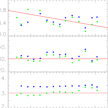
Figure 2: Redshift variations of $\langle G_{12}\rangle$ (top panel), Doppler parameter, $\langle b\rangle$ (middle panel) and $\langle lg(N_{HI})\rangle$ (bottom panel) for samples $S^{13}_{18}$ (blue points) and $S^{12}_{14}$ (green points). Mean values (34) and fit (32) are plotted by straight lines.

4.1 Redshift variations of the mean observed characteristics

Redshift variations of two observed characteristics of absorbers, $\langle b\rangle$, and $\langle lgN_{HI}\rangle$, are plotted in Fig. 2. For both samples $S_{14}^{12}$ and $S_{18}^{13}$, the mean values $\langle b\rangle$ and $\langle lgN_{HI}\rangle$ surprisingly weakly vary with redshift,

$$\langle b\rangle=(28.6\pm 1.6){\rm km}/{\rm s},\quad\langle b\rangle=(31.7\pm 1.6){\rm km}/{\rm s},$$ (34)

$$\langle lgN_{HI}\rangle=(13.1\pm 0.22),\quad\langle lgN_{HI}\rangle=(13.6\pm 0.06),$$

respectively. At the same time, the mean Doppler parameter systematically shifts from $\langle b\rangle=(25.6\pm 2.9)$km/s for the sample $W^{14}_{12}$ up to $\langle b\rangle=(38.4\pm 2.7)$km/s for 660 absorbers with $N_{HI}\geq 10^{14}{\rm cm}^{-2}$ what indicates a weak correlation of observed properties of absorbers. Detailed discussion of observed characteristics of absorbers can be found in Kim, Cristiani & D’Odorico (2002), Kim et al. (2002).

The small variations of $\langle b\rangle$ with the redshift are accompanied by similar small variations of dispersion $\sigma_{b}\sim 0.5\langle b\rangle$ which also do not exceed $\sim$ 8%. This fact indicates that the broad distribution function of $b$ is weakly dependent upon the redshift. The same is valid for the depth of potential wells, $\langle\Delta\Phi\rangle$ (14), and illustrates a correlation between the DM column density, $q$, and the overdensity of absorbers, $\delta$ described by (20). The nature of such a weak redshift evolution of these statistical characteristics of absorbers remains a mystery.

The function $\langle G_{12}\rangle/G_{0}$ is also plotted in Fig. 2 together with the rough fit (32). Its weak redshift dependence is a natural consequence of the weak redshift variations of $\langle b\rangle$ and $\langle lgN_{HI}\rangle$. Its deviations from (32) correlate with the absorbers distribution plotted in Fig 1 .

4.2 Redshift variations of the mean DM column density, overdensity and entropy of absorbers

Other characteristics of absorbers depend upon the physical model. For the model discussed in Sec. 2 (Eq. 20) with the function $\langle G_{12}\rangle$ (22, 32) the redshift variations of the mean DM column density, $\langle\xi\rangle$, the mean entropy and overdensity, $\langle F_{s}\rangle$ and $\langle\delta\rangle$, are plotted in Fig. 3.

The mean DM column density of absorbers, $\langle q\rangle\,\&\,\langle\xi\rangle\approx\langle q\rangle(1+z)^{2}$, is the most stable parameter. In principle, $\langle\xi\rangle$ does not change due to the formation and merging of absorbers and due to their transverse compression and/or expansion (DD02). The differences between the expected and measured $\langle\xi\rangle$ characterize, in fact, the influence of disregarded factors, mainly the completeness and representativity of the samples, the pancake relaxation and the scatter of the function $G_{12}$.

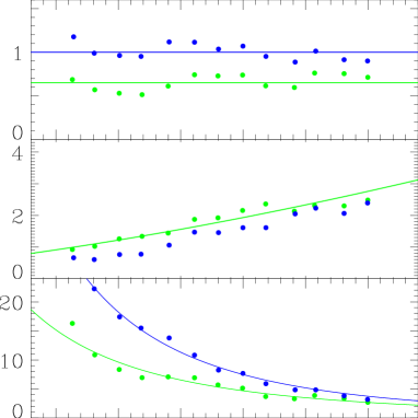
Figure 3: Functions $\langle\xi\rangle=(1+z)^{2}\langle q\rangle$ (top panel), $\langle F_{s}\rangle$ (middle panel) and the overdensity $\langle\delta\rangle$, (bottom panel) are plotted vs. redshift, $z$, for samples $S_{14}^{12}$ (green points), and $S_{18}^{13}$ (blue points). Fits (35, 36) are plotted by lines.

As is seen from comparison of Fig. 1 and Fig. 3, for both samples $S_{18}^{13}$ and $S_{14}^{12}$ variations of measured $\langle\xi(z)\rangle$ around the mean values

$$\langle\xi\rangle\approx(1.\pm 0.09),\quad\langle\xi\rangle\approx(0.65\pm 0.09)\,,$$ (35)

are roughly correlated with the redshift distribution of absorbers plotted in Fig. 1 what emphasizes the limited representativity of the sample used in the analysis. At small redshifts, $z\leq$ 2, the influence of the observational restrictions (Sec. 2.5) increase the measured value of $\langle\xi\rangle$.

For the sample $S_{14}^{12}$ the measured $\langle\xi(z)\rangle\approx 0.65$ is close to the expected value $\langle\xi(z)\rangle\approx 0.82$ what verifies the choice of the amplitude of $\langle G_{12}\rangle$ in (32). However, the estimates of $\langle\xi(z)\rangle$ depend also upon the choice of the amplitude of initial perturbations, $\tau_{0}$ (12), known only with a moderate precision. For the samples $S_{18}^{13}$ , $\langle\xi(z)\rangle$ increases due to the rejection of weaker absorbers in this sample.

For both samples, $S_{14}^{12}\,\&\,S_{18}^{13}$, the minimal DM column density is found to be $q_{min}\sim 10^{-2}$ and it only weakly depends upon the redshift. This result is especially sensitive to the random noise, it is based on poor statistic and is not reliable because our fit of $\langle G_{12}\rangle$ provides a reasonable description for the sample as a whole only. This value is smaller than the estimate $\langle q_{thr}\rangle\approx 3\cdot 10^{-2}$ (54) obtained in Sec. 6.3 from the analysis of redshift distribution of absorbers. This disagreement requires more detailed investigation and, perhaps, redefinition of the factors $G_{0}$, $\Theta_{H}$ and $\Theta_{\delta}$ .

As is seen from Fig. 3, the redshift variations of functions $\langle\delta\rangle$ and $\langle F_{s}\rangle$ characterizing the overdensity of DM component and entropy of gaseous component for both samples $S_{18}^{13}$ and $S_{14}^{12}$ can be roughly fitted as follows:

$$\langle\delta\rangle\approx 7.5\zeta^{-3.1},\quad\langle\delta\rangle\approx 4.7\zeta^{-2.5}\,,$$ (36)

$$\langle F_{s}\rangle\approx 1.93\zeta^{1.6},\quad\zeta=(1+z)/4\,.$$

These fits emphasize the general tendencies of absorbers evolution. Comparison with the background density (2) and entropy (5) shows that the mean density of absorbers weakly depends on the redshift and the mean entropy weakly increases with time. These results indicate that our sample is dominated by long lived relaxed absorbers.

These estimates may be rescaled according to (21).

4.3 The mean size of absorbers

Our model of absorbers ( see Sec. 2) allows also to estimate roughly the real size of absorbers along the line of sight, $\Delta r$. Due to the strong correlation between $q$ and $\delta$, this size should be obtained by averaging $\Delta r$ as given by (7). For the model parameters given in (33) and for both samples, $S_{14}^{12}$ and $S_{18}^{13}$, we have

$$\langle\Delta r\rangle\sim(80-100)h^{-1}{\rm kpc}\,,$$ (37)

and this size increases up to $\sim 150h^{-1}$ kpc for weaker absorbers of the sample $W_{14}^{12}$. For all samples the PDFs of the sizes are similar to the Gaussian function with a dispersion $\sigma_{r}\sim 0.5\langle\Delta r\rangle$.

The mean size of absorbers in the redshift space is associated with the Doppler parameter, $b$, as follows:

$$\langle\Delta r_{b}\rangle=2\langle b\rangle/H(z)\approx 130h^{-1}{\rm kpc}\left({4\over 1+z}\right)^{3/2}\sqrt{0.3\over\Omega_{m}}\,.$$

As usual, it is larger than that in the real space (37). This difference agrees with the domination of relaxed gravitationally bound absorbers in the sample.

The expected mean transverse size of absorbers is comparable with their Lagrangian size along the line of sight and was roughly estimated in DD02 as

$$\langle\Delta r_{t}\rangle\approx 5.2{l_{v}\tau^{2}\over 1+z}\approx{0.6l_{v}\over(1+z)^{3}}\approx 300h^{-1}{\rm kpc}\left({4\over 1+z}\right)^{3}\,.$$ (38)

Difference between estimates $\langle\Delta r\rangle$ and $\langle\Delta r_{t}\rangle$ agrees with expectations of the Zel’dovich theory and indicates that such absorbers could be unstable with respect to the disruption into a system of denser less massive clouds with $\Delta r_{t}\sim\Delta r$ (see, e.g., Doroshkevich 1980; Vishniac 1983).

4.4 The mean matter fraction accumulated by absorbers and the mean absorber separation

The mean matter fraction accumulated by absorbers, $\langle f_{abs}(z)\rangle$, and the mean absorber separation, $\langle D_{sep}(z)\rangle$, defined by (8 & 9), are plotted in Fig. 4 for the samples $W_{14}^{12}$, $S_{14}^{12}$ & $S_{18}^{13}$. The estimates of $\langle f_{abs}(z)\rangle$ are sensitive to small measured line separations, $\Delta z\sim 10^{-4}$, which are unreliable. For richer absorbers of the sample $S_{18}^{13}$, the estimates of $f_{abs}(z)$ based on the expression (9) are also unreliable because they neglect the transverse compression and expansion of matter and formation of high density clouds. So, the representativity and precision of measured $\langle f_{abs}(z)\rangle$ are limited. The estimates of $\langle D_{sep}(z)\rangle$ are less sensitive to the first factor but are also influenced by the second one. The random scatter of the measured $\langle f_{abs}(z)\rangle$ and $\langle D_{sep}(z)\rangle$ could be caused by the limited representativity of the samples at small and higher redshifts.

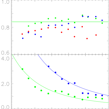
Figure 4: Mean fractions of matter accumulated by absorbers, $\langle f_{abs}\rangle$, (top panel) and the mean absorber separations, $\langle D_{sep}\rangle$, (bottom panel), are plotted vs. redshift, $z$, for samples $W_{14}^{12}$ (red points), $S_{14}^{12}$ (green points), and $S_{18}^{13}$ (blue points). Fits (39) are plotted by solid and dashed lines.

In spite of uncertainties these results are interesting in some respects. Thus, the regular growth of $\langle f_{abs}(z)\rangle$ and decrease of $\langle D_{sep}(z)\rangle$ with redshifts for the sample $S_{18}^{13}$ indicate the progressive disruption of richer absorbers and their transformation into system of high density clouds. Indeed, due to small cross–section of such clouds, they are rarely cross the line of sight and their formation increases the separation of richer observed absorber and even can decrease the measured $\langle f_{abs}\rangle$ for this sample.

Both the significant fraction of matter seen as numerous weaker absorbers in the sample $W_{14}^{12}$ and its weak redshift variation point in favor of the domination of absorbers merging as compared with the formation of new absorbers from the background matter. The merging remains unchanged the $\langle f_{abs}(z)\rangle$ but progressively increases $\langle D_{sep}(z)\rangle$ with time. These variations can be enhanced by the observational restrictions, $N_{HI}\geq N_{thr}$, discussed in Sec 2.5 .

For all samples the fraction $\langle f_{abs}(z)\rangle\sim 0.8$ exceeds the theoretical expectation $\langle f_{abs}(z)\rangle\sim$ 0.5–0.6 for $z\simeq 3$ (DD02 and Sec. 7.6) and is close to the maximal fraction, $f_{max}\simeq 0.875$, which can be compressed in the Zel’dovich’ theory. This disagreement indicates the limited applicability of the one dimensional expression (9) and the limited precision of our model of absorbers. These results must be tested with richer samples of observed absorbers and by comparison with simulations.

As is well known, at redshifts $z\geq$ 4 the absorbers begin to overlap and their separation becomes problematic. Analysis of the evolution of the mean absorbers separation allows to estimate quantitatively this effect. For this purpose, we can compare the mean separation of absorbers at various redshifts, $\langle D_{sep}(z)\rangle$, given by (8) with the mean Doppler parameter which characterizes the observed thickness of absorbers. For samples $S_{14}^{12}$ and $S_{18}^{13}$ these parameters are roughly fitted by power laws:

$$\langle D_{sep}\rangle\approx\left({4\over 1+z}\right)^{2.7}h^{-1}{\rm Mpc},\quad\approx\left({5.3\over 1+z}\right)^{2.7}h^{-1}{\rm Mpc}\,,$$

$${H_{0}\langle D_{sep}\rangle\over\langle b\rangle}\approx\left({6.1\over 1+z}\right)^{2.6},\quad{H_{0}\langle D_{sep}\rangle\over\langle b\rangle}\approx\left({8\over 1+z}\right)^{2.9}\,,$$ (39)

respectively.

These results verify that at $z\geq$ 4 absorbers effectively overlap and the system of individual absorbers is transformed into continuous absorption imitating the Gunn–Peterson effect.

4.5 Distribution functions of absorber parameters

The observed probability distribution function, PDF, of the DM column density of absorbers can be compared with the expected one (10). However, we have no theoretical expression for the PDFs of the Doppler parameter, overdensity and entropy of absorbers because the action of random factors cannot be satisfactory described.

Indeed, the relaxation of DM pancakes depends upon unknown internal structure of pancakes, the adiabatic compression and/or expansion of an absorber changes its overdensity and temperature. On the other hand, the radiative cooling and bulk heating lead to the drift of the gas entropy and overdensity but leaves unchanged the depth of potential well formed by DM distribution. Merging of pancakes increases more strongly the depth of potential well and the gas entropy but the overdensity of the gaseous component increases only moderately. All the time, the temperature and overdensity of trapped gas are rearranged in accordance with the condition of hydrodynamic equilibrium across the pancake.

Because of this, our discussion of absorbers evolution has only phenomenological character. The PDF of the DM column density, $N_{q}$, is plotted in Fig. 5 for the sample $S_{14}^{12}$ together with the fits (10) and (40). The distribution functions of the reduced Doppler parameter, $\upsilon$, are plotted in Fig. 5 for samples $S_{18}^{13}$ and $S_{14}^{12}$ together with the Gaussian fits.

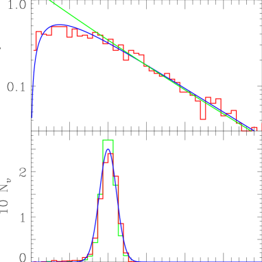
Figure 5: Top panel: PDFs of the DM column density, $N_{q}$, for the sample $S_{14}^{12}$. Fits (10) and (40) are plotted by green and blue lines. Bottom panel: PDF $N_{\upsilon}$, for the samples $S_{14}^{12}$ (red line) and $S_{18}^{13}$ (green line). Gaussian fit is plotted by blue line.

4.5.1 Distribution functions of the DM column density

The PDF for the DM column density of pancakes, $N_{q}(q)$, plotted in Fig. 5 for samples $S_{14}^{12}$ is the most interesting because it can be compared with the theoretically expected PDF (10) which, in particular, is sensitive to the coherent length of initial density field, $q_{0}$. As is seen from (10), the PDF $N_{q}(\xi)$, with $\xi\approx q(1+z)^{2}$, does not depend on the redshift and, so, the joint PDF can be obtained for absorbers observed at all redshifts.

For $\xi\geq 0.5\langle\xi\rangle$, the PDF plotted in Fig. 5 is well fitted by the function (10) for $q_{0}=0$ and $\langle\xi\rangle=$ 0.57 what is close to $\langle\xi\rangle=$ 0.65 (35). The deficit of observed absorbers with $\xi\leq\langle\xi\rangle$ can be related to incompleteness of the observed sample for small $\xi$. This result verifies the self consistency of the physical model used here and the Gaussianity of initial perturbations.

However, as it is seen from (10), this deficit of weaker absorbers can be related also to the suppression of the formation of poorer pancakes caused by the correlations of small scale initial perturbations and Jeans damping described by the parameter $q_{0}$ in (10). Indeed, the observed PDF is well fitted also by the function

$$N_{q}=0.18~{}{{\rm erf}(\sqrt{y})\over\sqrt{y}}{\exp(-y)\over(1+0.53/y)},\quad y=1.15{\xi\over\langle\xi\rangle}\,,$$ (40)

what is consistent with rough estimate $q_{0}\sim$ 0.05. This value depends on the statistics of absorbers at small $\xi\leq\langle\xi\rangle$ and can be considered as an upper limit of $q_{0}$ only.

4.5.2 Distribution functions of the reduced Doppler parameter

As was noted above, the theoretical description for the PDFs of the reduced Doppler parameter, overdensity and entropy of the gas is problematic because they depend upon many random factors. Therefore, here we will restrict our analysis to the fits of observed PDFs, $N_{\upsilon}$, taking also into account the correlations of the measured $\xi,\,b,\,\delta\,\&\,F_{s}$.

To adjust the reduced characteristics of pancakes introduced in Eq. (23), we will minimize the correlation of $\xi$ with $\upsilon,\,\Delta,\,\&\,S$. For the sample $S_{14}^{12}$, the adjusted reduced characteristics are defined as follows:

$$\gamma=1.8,\quad\upsilon=\ln(\beta\xi^{-0.44})\,,$$

$$\Delta=\ln[(1+z)^{3}\delta~{}\xi^{-1.1}]=\ln\delta_{0}-2\upsilon\,,$$ (41)

$$S=\ln[(1+z)^{-2}F_{s}\xi^{-0.15}]=const.+3.33~{}\upsilon\,.$$

These expressions correspond to Eq. (23) with the effective power index of compressed DM component $\gamma=1.8$. For the sample $S_{18}^{13}$ we have $\gamma=2.1$. Both values are close to $\gamma=2$ discussed in Sec. 2.3.1 . With such definition, we get the negligible correlations, $\leq 0.01$, between $\xi$ and other reduced characteristics and a strong correlation $\approx$ 1 between $\upsilon$ and $\Delta\,\&\,S$. The distribution function $N_{\upsilon}$ plotted in Fig. 5 is well fitted by the Gauss function with $\langle\upsilon\rangle=0.81\pm 0.04,~{}\sigma_{\upsilon}\approx 0.11\langle\upsilon\rangle$  what is consistent with the assumption of approximate equilibrium of majority of the observed absorbers.

These results mean that, in fact, the joint action of all random factors is characterized by the one random function $\upsilon$ which can be directly expressed through the observed parameters as follows

$$\upsilon\approx 0.48\ln~{}\beta-0.15\ln(N_{HI}/N_{0}/\delta_{0}),\quad\gamma=1.8\,.$$ (42)

More detailed analysis requires the discrimination of subpopulations of absorbers with different evolutionary histories.

4.6 Three subpopulations of absorbers

Table 2: Parameters of three subpopulations of absorbers for the sample $S_{14}^{12}$

	$N_{abs}$	$\langle f_{s}\rangle$	$\langle lgN_{HI}\rangle$	$\langle b\rangle$	$r_{bH}$	$\gamma$	$\langle\upsilon\rangle$
full	4369	1.00	13.1	29	0.30	1.8	0.8
sh	1940	0.44	13.0	37	0.33	1.8	1.0
cl	1664	0.38	13.5	23	0.67	1.6	0.6
exp	765	0.18	12.3	18	0.42	3.5	1.3

$f_{s}$ is the fraction of absorbers in a subpopulation, $r_{bH}$ is the linear correlation coefficient of $b$ and log$N_{HI}$.

As a first step of more detailed investigation of absorbers evolution, we can approximately separate three subpopulations of absorbers with different overdensities and entropies. Due to continuous distribution of both $\delta\,\&\,F_{s}$ for the full samples and because both these values depend upon unknown random factors (21), the separation is quite arbitrary and characteristics of subpopulations depend upon the sample used in the analysis and the parameters (33). Even so, the redshift variation of mean parameters of subpopulations allows to trace roughly their evolutionary history and to describe the main stages of absorbers formation and evolution.

The first subpopulation, let us call it ”sh”, with $\delta\geq$ 1 and $F_{s}\geq$ 1 is formed due to the merging and shock compression. The second one, called here ”cl”, includes low entropy absorbers with $\delta\geq$ 1, $F_{s}\leq$ 1 . The third one, called here ”exp”, contains peculiar absorbers with $\delta\leq$ 1.

This choice of the threshold parameters allows to separate absorbers formed and observed at the same redshifts, $z_{f}\approx z_{obs}$. However, due to evolution of the background density (2) and entropy (5), the functions $\delta\,\&\,F_{s}$ defined by (20) are shifted with time even when the overdensity and entropy of a long lived absorber are not changed. This shift leads to some artificial intermixture of subpopulations.

For the sample $S^{12}_{14}$ the mean parameters of these subpopulations are listed in Table 2, where $r_{bH}$ is the linear correlation coefficient of $b$ and $\lg N_{HI}$. Redshift variations of $\langle b\rangle$, $\langle lgN_{HI}\rangle$, $\langle F_{s}\rangle$, $\langle\delta\rangle$, $\langle q\rangle$, $\langle\xi\rangle$ and the relative number fractions of absorbers in these subpopulations, $\langle f_{m}\rangle$, are plotted in Figs. 6 & 7 and given in (43, 44 & 45).

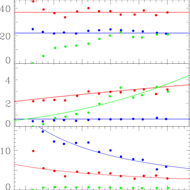
Figure 6: The mean Doppler parameter, $\langle b\rangle$ (top panel), the mean entropy, $\langle F_{s}\rangle$ (middle panel), and the mean overdensity $\langle\delta\rangle$ (bottom panel), are plotted vs. redshift, $z$, together with fits (43, 44, & 45) for the ”sh” (red), ”cl” (blue) and ”exp” (green) subpopulations of the sample $S_{14}^{12}$ .

The subpopulation ”sh” is composed of the richest and hottest absorbers with

$$\langle lgN_{HI}\rangle\approx 13.0\pm 0.4,\quad\langle b\rangle\approx(37\pm 2.7)km/s\,,$$ (43)

$$\langle\xi\rangle\approx 0.8\pm 0.15,\quad\langle F_{s}\rangle\approx 3.0\zeta^{0.6},\quad\langle\delta\rangle\approx 3.75/\zeta\,,$$

where $\zeta=(1+z)/4$. As is seen from Fig. 7, for this subpopulation the decrease of the relative number fraction of absorbers, $\langle f_{m}\rangle$, with $z$ is accompanied by the growth of the DM column density, $\langle q\rangle$. Such variations are typical for absorbers formed due to pancake merging and strong shock compression of the matter.

The subpopulation ”cl” includes absorbers with

$$\langle lgN_{HI}\rangle\approx 13.5\pm 0.37,\quad\langle b\rangle\approx(23.1\pm 1.1){\rm km}/{\rm s}\,,$$ (44)

$$\langle\xi\rangle\approx 0.69\pm 0.1,\quad\langle F_{s}\rangle\approx 0.6\pm 0.08,\quad\langle\delta\rangle\approx 8.7\zeta^{-1.6}\,.$$

Such behavior of the mean characteristics indicates that this subpopulation can be dominated by absorbers formed in low entropy regions at $z_{f}\sim z_{obs}$ due to adiabatic and weak shock compression. Such compression provides higher overdensity than the strong shock compression and does not change the entropy of compressed matter. For these absorbers the radiative cooling can also be more important. This subpopulation includes also some fraction of long lived absorbers formed at $z_{f}>z_{obs}$ due to merging and strong shock compression. This intermixture is caused by redshift variations of background parameters (2) and (5).

The peculiar subpopulation ”exp” accumulates poorer absorbers with

$$\langle lgN_{HI}\rangle\approx 12.3\pm 0.3,\quad\langle b\rangle\approx(18\pm 5.4){\rm km}/{\rm s},$$ (45)

$$\langle q\rangle\approx 1.1\cdot 10^{-2},\quad\langle F_{s}\rangle\approx 2.1\zeta^{2.5},\quad\langle\delta\rangle\approx 0.6\pm 0.08\,.$$

Such behavior of $\langle q\rangle,\,\langle\delta\rangle\,\&\,\langle F_{s}\rangle$ shows that these absorbers could be related to the unstable poorer pancakes formed within low density regions (see, e.g., Zhang et al. 1998). They are observed mainly at higher redshifts, they expand together with the background and disappear at low redshifts. Large values of the factor $\gamma=$ 3.5 and of the reduced Doppler parameter $\langle\upsilon\rangle=$ 1.3 (Table 2), verify the peculiar character of this subpopulation.

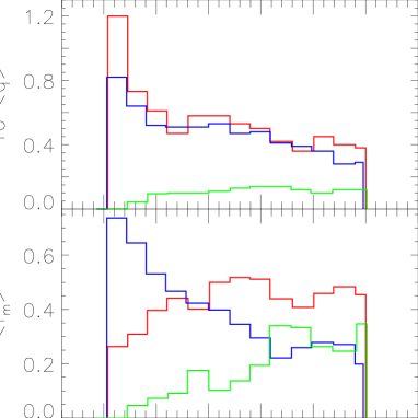
Figure 7: The DM column density (top panel) and the relative number fractions of absorbers (bottom panel) for the ”sh” (red lines), ”cl” (blue lines) and ”exp” (green lines) subpopulations of the sample $S_{14}^{12}$ are plotted vs. redshift, $z$ .

Moreover, the analysis performed in Sec. 6.3 indicates that, for weaker absorbers dominating this subpopulation, at least the DM column density, $\langle q\rangle$, can be underestimated. This means that other parameters of the subpopulation can also be estimated unreliably. In particular, if these absorbers are unstable then the random factors become time dependent and the estimates (45) must be corrected. Fortunately, the fraction of such absorbers is small and its influence on other estimates is limited.

In spite of the quite arbitrary separation of subpopulations these results illustrate the action of evolutionary factors mentioned above. The objective character of the discrimination is seen from the comparison of observed parameters, $\langle lgN_{HI}\rangle$ and $\langle b\rangle$, and their linear correlation coefficient, $r_{bH}$, listed in Table 2 for the full samples and for the separated subpopulations.

These results confirm that majority of observed absorbers represent gravitationally bounded pancakes formed in the course of adiabatic and shock compression at $z_{f}\geq z_{obs}$. They demonstrate similarity of evolutionary history and generic origin of subpopulations ”sh” and ”cl”. More detailed statistical investigation of absorbers evolution requires finer discrimination of subpopulations and therefore richer set of observed absorbers is needed.

4.7 Absorbers as a test of background properties

Some absorbers characteristics can be used to estimate the redshift variations of mean properties of homogeneously distributed hydrogen (see, e.g., Hui & Gnedin 1997; Schaye et al. 1999, 2000; McDonald et al. 2001). Thus, weak redshift variations of $\langle F_{s}\rangle$ (44) suggest also weak redshift variations of $T_{bg}$ (2). However, such estimates are inevitably approximate and their significant scatter is caused by action of many factors discussed above.

To obtain more stable results Schaye et al. (1999, 2000) consider a cutoff at small $b$ in the distribution of $b(N_{HI})$. Indeed, relations (20) can be rewritten as follows:

$$b=b_{bg}\kappa_{b}^{3/8}\delta_{0}^{1/8}\left({F_{s}\over(1+z)^{2}}\right)^{9/16}\left({N_{HI}\over N_{0}}\right)^{1/4}\,.$$ (46)

Parameters $N_{0},\delta_{0},b_{bg}\,\&\,\kappa_{b}$ were defined by (2, 15, & 19). Evidently, for $F_{s}={\rm const.}$ this relation is identical to the equation of state $b^{2}={\rm const.}\delta^{2/3}$. It demonstrates that, for the subpopulation of absorbers formed at $z_{f}\approx z_{obs}$ with the same $F_{s}$, the observed parameters $z,b$ and $N_{HI}$ are strongly correlated and, for a given $N_{HI}$, $b$ decreases with $F_{s}$. However, statistics of absorbers near the cutoff is small, the action of factors discussed above erodes the cutoff and makes its interpretation less reliable.

For absorbers selected from the sample $S^{12}_{14}$ in four redshift intervals, $z\leq$ 2 $\leq z\leq$ 2.5 $\leq z\leq$ 3 $\leq z$, the boundary of the observed distribution $b(N_{HI})$ can be roughly fitted by the relation

$$b\approx b_{0}(1+z)^{-1}(N_{HI}/10^{12}cm^{-2})^{\gamma_{b}}\,.$$ (47)

For $z\leq$ 3 we have $\gamma_{b}\sim$ 0.25 that coincides with (46) but the value of $b_{0}\sim$ 22 km/s is $\sim$ 2 times smaller, what is expected from (46). This means that in the framework of the model under consideration the cutoff can be naturally related to a fraction of low entropy absorbers with $F_{s}\sim$ 0.3 rather then with $F_{s}\sim$ 1. These absorbers can be formed at $z_{f}\sim z_{obs}$ due to the adiabatic compression within low entropy regions or due to both adiabatic and shock compressions at redshifts $z_{f}\geq~{}1.5~{}z_{obs}$. For richer absorbers with $lgN_{HI}\geq$ 13 the radiative cooling is also more important. This explanation is quite consistent with the estimates (44).

At $z\geq$ 3 we have for the fit parameters $\gamma_{b}\sim$ 0.15–0.17, $b_{0}\sim$ 38km/s, what differs from (46). This difference can be partly related to the poor statistics at higher redshifts and to admixture of long lived absorbers formed at redshifts $z\geq$ 4 when stronger systematic and random variations of UV background are expected. In particular, at $z\sim$ 3 $HeII$ becomes ionized and the spectrum of UV background and the effective power–low index of the temperature–density relation are changed (Songaila 1998; Schaye et al. 2000; Theuns et al. 2002a, b).

These results demonstrate that, in the framework of model under consideration, the cutoff in the distribution of $b(N_{HI})$ can be explained but its interpretation is not so clear. The problem requires further investigation.

5 Walls at high redshifts

Majority of the rare absorbers with higher Doppler parameter, $b\geq$ (80 – 90)km/s and moderate column density of neutral hydrogen $N_{HI}\leq 10^{14.5}cm^{-2}$, can be identified with the embryos of richer structure elements which are seen now as rich walls in the observed galaxy distribution. The number of such absorbers is small and their statistical characteristics cannot be reliably determined. However, for 45 such absorbers with $b\geq$ 90km/s selected in 9 spectra at $1.8\leq z\leq 3.8$ we have

$$\langle lgN_{HI}\rangle\sim 13.2,\quad\langle\xi\rangle\sim 1.45,\quad\langle\delta\rangle\sim 6,\quad\langle F_{s}\rangle\sim 10\,,$$ (48)

and the mean comoving separation of such absorbers (8) is

$$\langle D_{sep}\rangle\approx(60\pm 20)\sqrt{0.3/\Omega_{m}}h^{-1}{\rm Mpc}\,.$$ (49)

Such large separation suggests that these objects will retain their individuality up to small redshifts and, indeed, this separation is quite consistent with the mean wall separation $\langle D_{w}\rangle\approx(66\pm 13)h^{-1}$ Mpc measured for the SDSS EDR at $z=0$ (Doroshkevich, Tucker & Allam 2002). However, for smaller $b$, the number of absorbers rapidly increases and already for 139 absorbers with $b\geq$ 70km/s in 15 spectra the mean separation decreases to $D_{sep}\sim(40\pm 20)h^{-1}$Mpc.

These results show that the walls begin to form already at $z\sim 3$ and continue to form up to the present time. At the same time, the continuous distribution of all parameters of absorbers shows that at high redshifts the discrimination of walls and other structure elements is quite arbitrary. The problem deserves further investigation in a wider range of redshifts with a more representative sample of absorbers especially at high redshifts. Perhaps, such walls can be also observed in the galaxy distribution at high redshifts.

6 Redshift distribution of absorbers

In this section we compare the observed redshift distribution of absorbers with theoretical relations (26, 27) describing the expected redshift evolution of the 1D number density of DM pancakes, $n_{abs}$, due to their formation and merging. As is seen from these relations, the number density depends upon the cosmological model, moments of initial power spectrum and the threshold DM column density, $q_{thr}$. Therefore, to compare these expectations with observed absorbers distribution we have to select samples with $q\geq q_{thr}$ rather than to use samples with a minimal $N_{HI}$ discussed in Sec. 4. Such samples can be prepared using estimates of $q$ as given by (20) in spite of their unreliability for smaller $q$ (see Sec. 4.2, 6.3).

Both relations (26 & 27) are derived for the Gaussian initial perturbations. They depend on the redshift of absorbers only and, so, the impact of absorbers velocities and Doppler parameters on the resulting estimates is minimal. At $z\leq$ 4 these factors increase the scatter of measured $n_{abs}$ but only at $z\geq$ 4 – 4.5 they lead to a significant overlapping of absorbers (Sec. 4.4). The Jeans damping caused by the temperature of background is well described by (27) through the parameter $q_{0}$.

Four samples, namely, $Q_{14}^{50}$, $Q_{14}^{20}$, $Q_{14}^{10}$, and $Q_{14}^{01}$, with $q_{thr}=$ 0.05, 0.02, 0.01 & 0.001 were selected from 14 high resolution spectra. These samples contain 1554, 3299, 3998 and 4475 absorbers, respectively. Comparison of $q_{thr}$ used for the sample preparation with estimates of $\langle q_{thr}\rangle$ obtained from fits (26, 27) allows to test the self consistency of our physical model and the choice of parameters (33).

The richest sample $Q_{14}^{01}$ includes almost all lines and probably is incomplete. It can be used for comparison with results obtained for other samples. The sample $Q_{14}^{50}$ contains richer absorbers and is weakly sensitive to properties of small scale density field described by the parameter $q_{0}$ in (27). It is used to test the expression (26) and to estimate $\langle q_{thr}\rangle$ for such absorbers. The samples $Q_{14}^{20}$, $Q_{14}^{10}$ can be used for independent estimates of both $\langle q_{thr}\rangle$ and $q_{0}$. Of course, these estimates are statistical and averaged over the sample.

To test the sample dependence of our results we use the sample $Q_{18}^{10}$ with $q_{thr}=$ 0.01 selected from all 18 spectra. As compared with the sample $Q_{14}^{10}$ it contains $\sim$10% additional absorbers with $N_{HI}\geq 10^{13}cm^{-2}$. To demonstrate the possible variations of intensity of UV background we consider also the sample $W_{14}^{12}$ containing 2126 weaker absorbers with $N_{HI}\leq 10^{12}cm^{-2}$. Here we also use the sample of HST data (Bahcall et al. 1993, 1996; Jannuzi et al. 1998) which contains 1000 absorbers at $z\leq$ 1.5 . This sample is probably incomplete at least at $z\geq$ 1 .

6.1 Selection of Poissonian subsamples of absorbers

The first problem is the selection of Poissonian subsamples of absorbers and estimation of their mean number density at various redshifts. For this purpose, we use the measured redshift separations of neighboring absorbers, $\Delta z$, what partly attenuates the influence of selection effects inherent in individual spectra. Instead of separation we use the dimensionless comoving distance,

$$\Delta l=H_{0}\Delta z/H(z)\,,$$

and absorbers in the interval $z-dz<z<z+dz$, taken from the sample under investigation, are organized into an ‘equivalent single field’ by arranging the separations $\Delta l$ one after the other along the line of sight. For richer samples, distribution of absorbers separations obtained in this way is similar to the Poissonian one and the mean number density, $\langle n\rangle$, can be found by comparing the measured PDF with the differential or cumulative Poissonian PDFs:

$$dN/dx=\exp(-\langle n\rangle~{}x)/\langle n\rangle\,,$$ (50)

$$N=\exp(-\langle n\rangle~{}x)\,.$$ (51)

To decrease uncertainties and to estimate the actual scatter of these fits we rejected all points before the maxima of differential PDF and only more representative middle part of PDFs with the fraction of points $f\leq f_{thr}$ were used. The threshold fraction, $f_{thr}$, was varied between $f_{thr}=0.7$ and $f_{thr}=0.95$. Mean values and dispersions of the set of measurements with different $f_{thr}$ were taken as the actual value and scatter of $n_{abs}$. As a rule, the fit (51) of cumulative PDFs gives more stable estimates and smaller error bars than the fit (50) of differential PDFs. Both estimates of $n_{abs}$ are plotted in Figs. 8 & 9.

6.2 Variations of intensity of the UV background

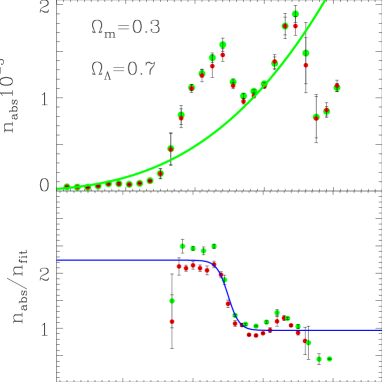
Figure 8: Top panel: redshift distribution of absorbers, $n_{abs}(z)$, found with fits (50) and (51) (red and green points) for the sample $W_{14}^{12}$. Fit (27) is plotted by green line. Bottom panel: redshift variations of $n_{abs}/n_{fit}$ for the same sample. Fit (52) is plotted by blue line.

For the sample $W_{14}^{12}$ the redshift distribution of absorbers is plotted in Fig. 8 together with the fit (27) which characterizes the expected redshift distribution of absorbers. The weak absorbers in this sample are especially sensitive to variations of intensity of the UV background radiation what is manifested by the strong variations of $n_{abs}$ in comparison with the smooth fitting curve. This effect can be enhanced by the incompleteness of the sample and the nonhomogeneity of redshift distribution of observed weaker absorbers. At $z\leq$ 2 the rapid decrease of $n_{abs}$ is caused by the influence of the threshold of the observed column density of neutral hydrogen, $N_{HI}\geq N_{thr}\approx 10^{12}cm^{-2}$, discussed in Sec. 2.5.

The observed variations of $\langle n_{abs}\rangle$ are well fitted by the function

$$\langle n_{abs}\rangle/n_{fit}=1.6+0.65~{}{\rm th}\left({2.5-z\over 0.16}\right)\,,$$ (52)

also plotted in Fig. 8. Similar variations with smaller amplitude are also seen for absorbers in other samples.

The column density of neutral hydrogen is proportional to $\Gamma_{\gamma}^{-1}$ and an increase of $\Gamma_{\gamma}$ shifts weak absorbers below the observational threshold. This means that the relation (52) can describe quite well the redshift dependence of variations of the UV background but their amplitude depends upon the distribution function of $N_{HI}$. Direct estimates show that the variations of the intensity by about 2 – 3 times described by (31) are consistent with the observed variation of $\langle n_{abs}\rangle$. As was noted in Sec. 2.6 the influence of these variations on the mean characteristics of absorbers can be partly compensated by variations of random factors $\Theta_{H}\,\&\,\Theta_{\delta}$.

Variations of the UV background at $z\sim 3$ were already detected by different methods (see, e.g., Songaila 1998; Scott et al. 2000; McDonald & Miralda–Escude 2001). This approach seems to be sufficiently perspective but quantitative results are sample dependent and must be tested with more representative and homogeneous samples of weak absorbers.

6.3 Redshift distribution of DM pancakes

In this Section we consider the redshift distribution of DM pancakes for the samples $Q_{14}^{50}$, $Q_{14}^{20}$, $Q_{14}^{10}$, and $Q_{14}^{01}$ prepared with $q_{thr}(z)\approx{\rm const.}$ for parameters (33). For the sample $Q_{14}^{10}$, the function $n_{abs}(z)$ is plotted in Fig. 9 together with the best fit (27) and the random scatter of observed points around the fit. At redshifts 1.8 $\leq z\leq$ 3.3 where the representativity of samples is better the scatter does not exceed $\sim$ 20% .

At redshifts $z\sim$ 1.5 – 2 the rapid growth of observed mean number density of absorbers

$$\langle n_{abs}\rangle\propto\left({1+z\over 2.7}\right)^{8}\,,$$ (53)

coincides with the expected one (30) and is naturally explained by the influence of observational threshold $N_{HI}\geq N_{thr}\approx 10^{12}cm^{-2}$. Such cutoff is not seen for the subpopulation of richer absorbers with $N_{HI}\geq 10^{14}cm^{-2}$ what verifies its connection with the observational threshold. The probable incompleteness of the sample of weak absorbers at $z\leq$ 1.5 enhances this rapid growth of $\langle n_{abs}\rangle$.

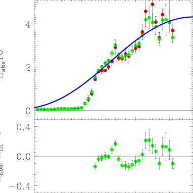
Figure 9: Top panel: redshift distribution of absorbers, $n_{abs}(z)$, found with fits (50) and (51) (red and green points) for the sample $Q_{14}^{10}$. Fit (27) is plotted by the blue line. Bottom panel: Differences between measured and fitted absorber distributions.

The best estimates of the fit parameters (27) for the samples $Q_{14}^{20}$, $Q_{14}^{10}$, and $Q_{14}^{01}$ are, respectively,

$$\langle q_{thr}\rangle\approx(3.3\pm 0.3)\cdot 10^{-2},\quad\langle q_{thr}\rangle\approx(3.1\pm 0.3)\cdot 10^{-2}\,,$$

$$\langle q_{thr}\rangle\approx(3.1\pm 0.3)\cdot 10^{-2}\,,$$ (54)

and for all three samples

$$q_{0}\approx(0.9\pm 0.1)\cdot 10^{-2}\,.$$ (55)

Here the formal errors of the fits are given.

To test the sample dependence of the results we analyzed in the same manner the sample $S_{18}^{10}$ selected with $q_{thr}$= 0.01 from all 18 spectra (4404 absorbers). In this case, the excess of absorbers with $N_{HI}\geq 10^{13}cm^{-2}$ and larger separations decrease the measured $n_{abs}$ and the resulting estimates are

$$\langle q_{thr}\rangle\approx(3.2\pm 0.3)\times 10^{-2},\quad q_{0}\approx(1.1\pm 0.12)\times 10^{-2}\,.$$

We see that such perturbations lead to moderate variations of both $\langle q_{thr}\rangle$ and $q_{0}$ .

Real precision of both estimates (54) and (55) depends upon several factors, mostly on the limited representativity of the sample and precision of estimates $\tau_{0}$ (12). As is seen from (27), we really evaluate the product $q_{thr}\tau_{0}^{-2}$ and $q_{0}\tau_{0}^{2}$, and, so, the real precision of both estimates (54) and (55) is not better than $\sim$ 20 – 30% .

As was noted in Sec. 2.4, the redshift distribution of absorbers with larger $q_{thr}$ is weakly sensitive to small scale correlations of perturbations and it can be fitted by the expression (26). Indeed, for samples $Q_{14}^{20}$ and $Q_{14}^{50}$ these distributions are well fitted by expression (26) with $\langle q_{thr}\rangle\approx$ 0.035 & 0.05, respectively, and the amplitude of the fit is only $\sim$ 1.2 – 1.3 times larger then what is expected in (26). However, already for the sample $Q_{14}^{10}$ the difference between expected and measured amplitudes of the fit (26) increases by up to $\sim$ 1.75 times.

These results show that the actual reliability and precision of our estimates (55) are limited due to limited representativity of the samples and limited precision of estimates of the amplitude $\tau_{0}$ (12). None the less, they suggest that:

1. The redshift distribution of absorbers is quite well fitted by relations (26) and (27) derived for the Gaussian initial perturbations.

2. The distribution of weaker absorbers is actually sensitive to the small scale cutoff of power spectrum described by the parameter $q_{0}\approx(0.9\pm 0.3)\cdot 10^{-2}$ .

3. Comparison of estimates (54) with $q_{thr}$ used for the sample selection indicates that, for weak absorbers with $q\sim 10^{-2}$, the expression (20) with parameters (33) underestimates the DM column density. However, for richer absorbers the divergence decreases to the quite moderate value ($\sim$ 10%).

The model as a whole and estimates of $q_{0}$ can be improved with richer sample of absorbers especially at high redshifts $z\geq$ 3.5 where the representativity of our samples is insufficient. However, as was noted in Songaila (1998) and Schaye et al. (2000), at $z\geq$ 3 the random variations of the UV background and the scatter of $\langle n_{abs}\rangle$ increase.

7 Summary and Discussion.

In this paper we continue the analysis initiated in Paper I and Paper II based on the statistical description of Zel’dovich pancakes (DD99, DD02). This approach allows to connect the observed characteristics of absorbers with fundamental properties of the initial perturbations without any smoothing or filtering procedures, to reveal and to illustrate the main tendencies of structure evolution. It demonstrates also the generic origin of absorbers and the Large Scale Structure observed in the spatial galaxy distribution at small redshifts.

We investigate the new more representative sample of $\sim$ 4 500 absorbers what allows us to improve the physical model of absorbers introduced in Paper I and Paper II and to obtain reasonable description of physical characteristics of absorbers. The progress achieved demonstrates again the key role of the representativity of observed samples for the construction of the physical model of absorbers and reveals a close connection between conclusions and observational database.

However, the representativity of this sample is not sufficient for the more detailed study of structure evolution. Further progress can be achieved with richer sample of observed absorbers.

7.1 Main results

Main results of our analysis can be summarized as follows:

1. The approach used in this paper allows to link the observed and other physical characteristics of Ly-$\alpha$ absorbers such as the overdensity and entropy of the gaseous component and the column density of DM component accumulated by absorbers.

2. The basic observed properties of absorbers are quite successfully described by the statistical model of DM confined structure elements (Zel’dovich pancakes). Comparison of independent estimates of the DM characteristics of pancakes confirms the self consistency of the physical model for richer absorbers. However, some characteristics of pancakes formation and evolution remain uncertain.

3. In the framework of this approach, all characteristics of absorbers can be expressed through two functions, $\xi\,\&\,\upsilon$, describing the systematic and random variations of absorber properties. They are directly expressed through the observed parameters, $z,\,N_{HI}\,\&\,b$.

4. The main stages of structure evolution are illustrated by separation of three subpopulations of absorbers with high and low entropy and low overdensity.

5. The absorbers with high Doppler parameter, $b\geq$ 90 km/s, can be naturally identified with the embryos of wall–like structure elements observed in the spatial distribution of galaxies at small redshifts.

6. The strong suppression of the mean number density of absorbers at $z\leq$ 1.8 can be naturally explained by the influence of the observational threshold $N_{HI}\geq~{}10^{12}{\rm cm}^{-2}$.

7. Redshift distribution of weaker absorbers indicates the probable systematic redshift variations of the UV background. They can be caused by the reionization of $HeII$.

8. The PDF of the DM column density and the redshift distribution of absorbers are consistent with Gaussian initial perturbations.

9. We estimate the spectral moment $m_{0}$ which in turn is linked with the cutoff of the power spectrum caused by the mass of dominant fraction of DM particles and the Jeans damping.

7.2 Variations of intensity of the UV background

The intensity of the UV background and its variations at redshifts $z\sim$ 2 – 3 were detected by different methods (see, e.g., Songaila 1998; Scott et al. 2000; McDonald &  Miralda-Escude 2001). However, the achieved precision of these estimates is limited. The variations of background temperature at these redshifts were also detected by Schaye et al. (2000) and McDonald et al. (2001).

The redshift variations of the mean number density of weak absorbers discussed in Sec. 6.2 can be naturally related to such variations caused by the reionization of HeII and possible variations of activity of quasars and other sources of UV radiation. They can be enhanced by the incompleteness and limited representativity of our samples and by the nonhomogeneous redshift distribution of observed absorbers.

However, these variations do not lead to appreciable variations of the mean absorbers characteristics discussed in Sec. 4 what indicates the complex character of absorbers evolution. The problem requires more detailed investigation using both observations and simulations.

7.3 Properties of absorbers

The physical model of absorbers introduced in Sec.2 links the measured $z$, $b$ and $lgN_{HI}$ with other physical characteristics of both gaseous and DM components forming the observed absorbers. Uncertainties in the available estimates of the background temperature and UV radiation and unknown parameters of the model restrict its applications. Fortunately, actions of these factors partly compensate each other, what allows us to obtain reasonable statistical description for majority of absorbers. The self consistency of this approach is confirmed by two independent estimates of the column density of DM pancakes. Numerical simulations can clarify action of unknown factors and improve the model.

Analysis of mean absorbers characteristics performed in Sec. 4 shows that the sample of observed absorbers is composed of pancakes with various evolutionary histories. We discuss five main factors that determine absorbers evolution after formation. They are: the transverse expansion and compression of pancakes, their merging, the radiative heating and cooling of compressed gas, and the disruption of structure elements into a system of high density clouds. The first two factors change the overdensity of DM and gas but do not change the gas entropy. Next two factors change both the gas entropy and overdensity but do not change the DM characteristics. Using the entropy and overdensity we can roughly discriminate three subpopulations of absorbers, illustrate the influence of these factors and correlations between absorbers characteristics.

Introduction of the reduced Doppler parameter, $\upsilon$, overdensity, $\Delta$, and entropy, $S$, allows to discriminate between the systematic and random variations of absorbers properties. The former ones are naturally related to the progressive growth with time of the DM column density of absorbers, $q(z)$, what can be described theoretically. On the other hand the action of random factors cannot be satisfactory described by any theoretical model. However, in the framework of our approach, the reduced parameters are found to be strongly correlated (41) and, in fact, the joint action of all random factors is summarized by one random function, $\upsilon$, directly expressed through the observed parameters (42). These results alleviate the problem of absorbers description and, perhaps, the modeling of the Ly-$\alpha$ forest based on the simulated DM distribution (Viel et al. 2002). However, estimates of the matter fraction accumulated by absorbers (Sec. 4.4) demonstrate that the model needs to be improved.

Estimates of the size of absorbers (Sec. 4.3) suggest a possible fast disruption of richer absorbers into a system of high density clouds, what is the first step of formation of dwarf galaxies.

7.4 Absorbers as elements of the Large Scale Structure of the Universe

The close connection of absorbers with the Large Scale Structure (LSS) of the Universe observed in the spatial galaxy distribution was demonstrated in numerical simulations and was recently confirmed by direct observations (Penton, Stocke & Shull 2002). Our results indicate the generic link of absorbers and DM Zel’dovich pancakes and demonstrate that the absorbers characteristics are consistent with Gaussian initial perturbations and the Harrison–Zel’dovich power spectrum. The possible identification of some absorbers with embryos of walls observed in the galaxy surveys at small redshifts shows that, perhaps, also a wider set of richer absorbers could be identified with the LSS elements at high redshifts.

7.5 Characteristics of the initial power spectrum

The amplitude and the shape of large scale initial power spectrum are approximately established by investigations of relic radiation and the structure of the Universe at $z\ll$ 1 detected in large redshift surveys such as the SDSS (Dodelson et al. 2002) and 2dF (Efstathiou et al. 2001). The shape of small scale initial power spectrum can be tested at high redshifts where it is not so strongly distorted by nonlinear evolution (see, e.g., Croft et al. 2002).

Recent discussions on the mass of dominant fraction of DM component and the shape of small scale initial power spectrum are focused on the formation of low mass halos in CDM simulations in comparison with observed low mass satellites (see, e.g., Colin, Avila-Reese & Valenzuela 2001; Bode, Ostriker & Turok 2001), and at the simulations of absorbers formation. Thus, Narayanan et al. (2000) estimate the low limit of this mass as $M_{DM}\geq$ 0.75 keV, while Barkana, Haiman & Ostriker (2001) increase this limit up to $M_{DM}\geq$ 1 – 1.25 keV.

Here we can compare these estimates with direct measurements of redshift distribution of absorbers. In fact, our estimates are related to two spectral moments of the initial power spectrum, $m_{-2}$ and $m_{0}$. The first of them depends mainly upon the large scale power spectrum and was independently estimated from the measured characteristics of observed galaxy distribution at small redshifts. Together with cosmological parameters, $\Omega_{m}$ and $h$, this moment defines the coherent length of initial velocity field, $l_{v}$, (6), used in Sec. 2.3 for discussion of properties of DM distribution. The second moment, $m_{0}$, depends upon the small scale power spectrum and the shape of transfer function. This means that the estimates of the mass of DM particles are model dependent even though our estimates of $q_{0}$ and spectral moments are based on the analysis of observations.

As was shown in DD99 and DD02, for the CDM and WDM models with the Harrison – Zel’dovich asymptotic of power spectrum, $p(k)\propto k$, and transfer functions, $T(k)$, given in Bardeen et al. (1986) the coherent length of initial density perturbations, $l_{\rho}$, and the parameter $q_{0}$ can be written as follows:

$$q_{0}=5{m_{-2}^{2}\over m_{0}},\quad l_{\rho}=q_{0}l_{v}\approx 0.34h^{-1}{\rm Mpc}\left({q_{0}\over 0.01}{0.2\over\Omega_{m}h}\right)\,,$$ (56)

$$m_{-2}=\int_{0}^{\infty}dx~{}xT^{2}(x)\approx 0.023,\quad m_{0}=\int_{0}^{\infty}dx~{}x^{3}T^{2}(x)\,,$$

$$x={k\over k_{0}},\quad k_{0}=\Omega_{m}h^{2}/{\rm Mpc},\quad l_{v}={1\over k_{0}\sqrt{m_{-2}}}={6.6\over\Omega_{m}h^{2}}{\rm Mpc}\,,$$

where $k$ is the comoving wave number.

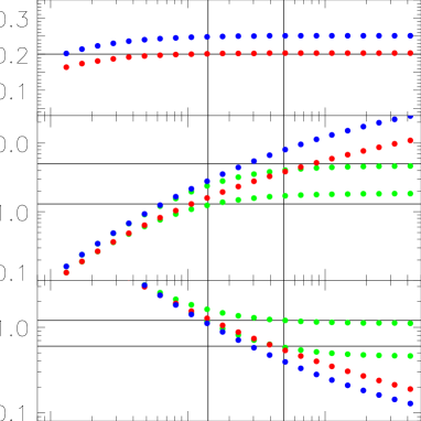
Figure 10: Spectral moments, $m_{-2}$ and $m_{0}$, and the parameter $q_{0}$ are plotted vs. $M_{DM}$ for the CDM (red points) and WDM (blue points) models with the damping factors $D_{W}$ (57) and with both damping factors, $D_{W}\,\&\,D_{J}$ (58) for $x_{J}=(2\,\&\,0.5)\cdot 10^{-2}$, (green points). Black lines show the observational restrictions (59).

For WDM particles the dimensionless damping scale, $R_{f}$, and the damping factor, $D_{W}$, are

$$R_{f}=0.2\left({\Omega_{m}h^{2}{\rm keV}}\over M_{DM}\right)^{4/3}\,,$$

$$D_{W}=\exp[-xR_{f}-(xR_{f})^{2}]\,,$$ (57)

(Bardeen et al. 1986). The Jeans wave number, $k_{J}$, and the damping factor, $D_{J}$, can be taken as

$$k_{J}^{-1}\approx 0.7b_{bg}(1+z)H^{-1}(z),\quad D_{J}\approx(1+x_{J}^{2}x^{2})^{-1}\,,$$ (58)

$$x_{J}=k_{0}/k_{J}\approx 2\cdot 10^{-2}\sqrt{\Omega_{m}h^{2}\over 0.13}\sqrt{4\over 1+z}\,{b_{bg}\over 16km/s}\,,$$

(see, e.g., Matarrese & Mohayaee 2002).

Variations of the spectral moments and $q_{0}$ with the mass of DM particle obtained by integration of the power spectrum with these damping factors are plotted in Fig. 10 for the CDM and WDM transfer functions and for $x_{J}=2\cdot 10^{-2}\,\&\,0.5\cdot 10^{-2}$. As is seen from this Fig., the low limit $q_{0}\geq 0.07\sqrt{x_{J}}$ caused by the Jeans damping (58), restricts the range of masses of DM particles detectable with this approach to $M_{DM}\leq$ (3 – 5)keV.

Our 1$\sigma$ estimates

$$q_{0}\approx(0.6-1.2)\cdot 10^{-2},\quad m_{0}\approx 0.15-0.5,$$

$$M_{DM}\approx(1.5-5){\rm keV}\,,$$ (59)

are close to those of Narayanan et al. (2000) and Barkana, Haiman & Ostriker (2001). They are based on absorbers with the redshifts $z\leq$ 3.5 where the scatter of measured $n_{abs}$ is minimal and, so, they weakly depend upon both the Doppler parameter and velocities of absorbers which essentially distort $n_{abs}$ at higher redshifts (Sec. 4.4).

There are plenty of possible candidates for the WDM particles with the mass $\sim$ 1 keV. They are, for example, the sterile neutrinos, majorons and even shadow particles. Detailed review of possible candidates can be found in Sommer-Larsen & Dolgov (2001) and Dolgov (2002). However, our estimates use the spectral moments and therefore do not forbid the existence of multicomponent heavy DM particles with both thermal and non-thermal (Lin et al. 2001) distributions with the same spectral moments $m_{-2}$ and $m_{0}$.

7.6 Reheating of the Universe

Recent observations of high redshift quasars with $z\geq$ 5 (Djorgovski et al. 2001; Becker et al. 2001; Pentericci et al. 2001; Fan et al. 2001) demonstrate clear evidences in favor of the reionization of the Universe at redshifts $z\sim$ 6 when the volume averaged fraction of neutral hydrogen is found to be $f_{H}\geq 10^{-3}$ and the photoionization rate $\Gamma_{\gamma}\sim(0.2-0.8)\cdot 10^{-13}s^{-1}$ . These results are consistent with those expected at the end of the reionization epoch which probably takes place at $z\sim$ 6. Extrapolation of the mean separation of absorbers discussed in Sec. 4.4 is consistent with these conclusions.

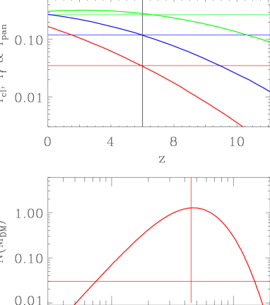
Figure 11: Top panel: expected redshift variations of the DM fraction accumulated by high density clouds, filaments and pancakes (red, green and blue lines), respectively, at $q_{0}=10^{-2}$. Bottom panel: the expected mass function of the DM clouds at $z=6$ and $q_{0}=10^{-2}$.

These results can be compared with expectations of the Zel’dovich approximation (DD02) for $q_{0}=10^{-2}$. The potential of this approach is limited since it cannot describe the nonlinear stages of structure formation and, so, it cannot substitute the high resolution numerical simulations. However, it describes quite well many observed and simulated statistical characteristics of the structure such as the redshift distribution of absorbers and evolution of their DM column density. This approach does not depend on the box size, number of points and other limitations of numerical simulations and it successfully augments them.

This approach allows to estimate the fractions of DM component accumulated by high density clouds, $f_{cl}$, filaments, $f_{f}$, and pancakes, $f_{pan}$, at different redshifts. These functions plotted in Fig. 11 for $q_{0}=10^{-2}$ show that at $z\sim$ 6 only $\sim$ 3.5% of the matter is condensed within the high density clouds which can be associated with luminous objects. This value can increase up to $\sim$ 5 – 6% with more correct description of the clouds collapse. At the same redshifts, $\sim$ 27% and $\sim$ 12% of the matter can be already accumulated by pancakes and filaments, respectively. These expectations are smaller than estimates of $\langle f_{abs}\rangle$ obtained in Sec. 4.4 .

The Zel’dovich approximation allows also to estimate the mass function of all structure elements (DD02) at different redshifts. For $q_{0}=10^{-2}$ and at $z\sim$ 6, this function is plotted in Fig. 11. For these $q_{0}$ and $z$, the mean DM mass of structure elements is expected to be $\sim 10^{12}M_{\odot}$ and the main mass is concentrated within clouds with $M_{cl}\sim 0.1\langle M_{cl}\rangle$. As is seen from Fig. 11, majority of the clouds have mass between $10^{-3}\langle M_{cl}\rangle$ and 10 $\langle M_{cl}\rangle$. The formation of low mass clouds with $M_{cl}\leq 10^{9}M_{\odot}$ is suppressed due to strong correlation of the initial density and velocity fields at scales $\leq l_{\rho}\sim 0.3h^{-1}$ Mpc (56). However, the numerous low mass satellites of large central galaxies can be formed in the course of disruption of massive collapsed clouds at the stage of their compression into thin pancake–like objects (Doroshkevich 1980; Vishniac 1983). The minimal mass of such satellites was estimated in Barkana, Haiman & Ostriker (2001).

This means that the investigation of absorbers observed at high redshifts should be supplemented by the study of properties of dwarf isolated galaxies and discrimination between such galaxies and dwarf satellites of more massive galaxies. It seems to be a perspective way to discriminate between models with the Jeans damping (58) and the damping caused by the mass of WDM particles, (57), and, in particular, between models with one and several types of DM particles.

Acknowledgments

AGD is grateful to Dr. S. Cristiani and Dr. T.S.Kim for the permission to use the unpublished observational data. This paper was supported in part by Denmark’s Grundforskningsfond through its support for an establishment of Theoretical Astrophysics Center and by the Polish State Committee for Scientific Research grant Nr. 2-P03D-014-17. AGD also wishes to acknowledge support from the Center of Cosmo-Particle Physics, Moscow. Furthermore, we wish to thank the anonymous referee for valuable discussion and many useful comments.

References

- [1993] Bahcall J.N. et al., 1993, ApJS., 87, 1.
- [1995] Bahcall J.N. et al., 1996, ApJ., 457, 19.
- [1986] Bardeen J.M., Bond J.R., Kaiser N., Szalay A., 1986, ApJ., 304, 15
- [2001] Barkana R., Haiman Z., Ostriker J.P., 2001, ApJ., 558, 482
- [2001] Becker R.H. et al. 2001, AJ, 122, 2850
- [1992] Bergeron J., Cristiani S., & Shaver P.A., 1992, A&A, 257, 417
- [1997] Bi H., & Davidsen A.F., 1997, ApJ., 479, 523
- [1981] Black J.H., 1981, MNRAS, 197, 553
- [2001] Bode P., Ostriker J.P. & Turok N, 2001, ApJ., 556, 93
- [2001] Bond R., Wadsley J.W., 1997, in ”Structure and Evolution of the IGM from QSO Absorption Line Systems”, Eds. P.Petitjean, S.Charlot, Editions Frontiers, Paris, p. 143
- [2001] Choudhury R., Padmanabhan T. & Srianand R., 2001, MNRAS, 322, 561
- [2001] Choudhury R., Srianand R. & Padmanabhan T., 2001, ApJ, 559, 29
- [1993] Coles P., Melott A., & Shandarin S., 1993, MNRAS, 289, 37
- [2001] Colin P., Avila-Reese V., & Valenzuela O., 2001, ApJ., 542, 622
- [1995] Cristiani S., D’Odorico V., 2000, AJ, 120, 1648
- [1998] Croft R.A.C., Weinberg D.H., Katz N., & Hernquist L., 1998, ApJ., 495, 44
- [2001] Croft R.A.C. et al., 2001, ApJ., 557, 67
- [2002] Croft R.A.C. et al., 2002, astro-ph/00132324
- [1998] Davé R., Hernquist L., Katz N., Weinberg D.H., 1999, ApJ., 511, 521,
- [1999] Demiański M. & Doroshkevich A., 1999, MNRAS., 306, 779, (DD99).
- [2000] Demiański M., Doroshkevich A.G., Müller V., & Turchaninov V.I., 2000, MNRAS, 318, 665
- [2001] Demiański M., Doroshkevich A.G., & Turchaninov V.I., 2001, MNRAS, 318, 1177, (Paper I)
- [2001] Demiański M., Doroshkevich A.G., & Turchaninov V.I., 2001, MNRAS, 318, 1189, (Paper II)
- [2002] Demiański M. & Doroshkevich A., 2002, astro-ph/0206282, (DD02)
- [2001] Djorgovski S.G., Castro S., Stern D., Mahabal A.A., 2001, ApJ., 560, L5
- [2002] Dodelson S. et al., 2002, ApJ, 572, 140
- [2002] Dolgov A., 2002, Phys.Rep., in press, hep=ph/0202122
- [1980] Doroshkevich, A.G., 1980, SvA., 24, 152
- [2002] Doroshkevich, A.G., Tucker, D.L. & Allam S., 2002, astro-ph/0206301
- [2001] Efstathiou G. et al., 2001, astro-ph/0109152
- [2001] Fan X. et al., 2001, astro-ph/0111184, ApJ., in press
- [1996] Gnedin N.Y. & Hui L., 1996, ApJ, 472, L73
- [2002] Gnedin N.Y. & Hamilton A.J.S., 2002, MNRAS, 334, 107
- [1993] Giallongo E., Cristiani S., Fontana A., & Trevese D., 1993, ApJ., 416, 137
- [1995] Hu E.M., Tae-Sun K., Cowie L., & Songaila A., 1995, AJ, 110, 1526
- [1997] Hui L., Gnedin N.Y., 1997, MNRAS, 292, 27
- [1997] Hui L., Gnedin N.Y. & Zhang Yu., 1997, ApJ, 486, 599
- [1999] Hui L., Rutledge R.E., 1999, ApJ, 517, 541
- [1986] Ikeuchi S., Ostriker J.P, 1986, ApJ., 301, 522.
- [1998] Jannuzi B.T. et al. ApJS. 1998, 118, 1
- [1994] Jacobsen P., et al. 1994, Nature, 370, 35
- [1997] Khare P. et al., Bechtold J., 1997, MNRAS, 285, 167.
- [2002] Kim T.S., Cristiani S., & D’Odorico S., 2002, A&A, in press, astro-ph/0201204
- [2002] Kim T.S., Carswell R.F., Cristiani S., D’Odorico S. & Giallongo E., 2002, MNRAS, in press, astro-ph/0205237
- [1997] Kirkman D., & Tytler D., 1997, ApJ., 484, 672.
- [1996] Kulkarni V.P. et al., 1996, MNRAS, 279, 197
- [1995] Lanzetta K.M., Bowen D.V., Tytler D., & Webb J.K., 1995, ApJ., 442, 538.
- [1996] Le Brune V., Bergeron J., & Boisse P., 1996, A&A, 306, 691
- [2001] Lin W.B., Huang D.H., Zhang X., Brandenberger R., 2001, Phys.Rev.Lett. 86, 954
- [1996] Lu L., Sargent W.L.W., Womble D.S., Takada-Hidai M., 1996, ApJ., 472, 509
- [2002] Matarrese S. & Mohayaee R., 2002, MNRAS, 329, 37
- [2000] McDonald P. et al., 2000, ApJ., 543, 1
- [2001] McDonald P. & Miralda-Escude J., 2001, ApJ., 549, L11
- [2001] McDonald P. et al., 2001, ApJ., 562, 52
- [1990] McGill C., 1990, MNRAS, 242, 544
- [2000] Narayanan V. et al., 2000, ApJ., 543, L103
- [1981] Oort J.H., 1981, Astr.Astrophys., 94, 359.
- [1984] Oort J.H., 1984, Astr.Astrophys., 139, 211.
- [2001] Pentericci L. et al., 2001, astro-ph/0112075
- [2002] Penton S.V., Stocke J.T., & Shull J.M, 2002, ApJ., 565, 720
- [1998] Rauch M., 1998, Ann.Rev.Astr.Astrophys., 36, 267
- [1995] Rodriguez-Pascual P.M., de la Fuente A., 1995, ApJ., 448, 575.
- [1980] Sargent, W.L.W., Young, P.J., Boksenberg, A. & Tytler, D., 1980, Ap.J.Suppl, 42, 41
- [1999] Schaye J., Theuns T., Leonard A. & Efstathiou G., 1999, MNRAS, 310, 57
- [2000] Schaye J.et al., 2000, MNRAS, 318, 817
- [2000] Scott J., Bechtold J., Dobrzicki A. & Kulkarni V.P., 2000, ApJSupl, 130, 67
- [1989] Shandarin S., Zel’dovich Ya.B., 1989, Rev.Mod.Phys., 61, 185
- [1995] Shandarin S. et al., 1995, Phys.Rev.Let., 75, 7
- [1996] Shectman S.A. et al., 1996, ApJ., 470, 172.
- [2001] Sommer-Larsen J. & Dolgov A., 2001, ApJ., 551, 608
- [1998] Songaila A., 1998, AJ., 115, 2184
- [2001] Stoughton C. et al., 2001, AJ., 123, 485
- [2002] Theuns T., Leonard A., Schaye J., Efstathiou G., 1999, MNRAS, 303, L58
- [2002] Theuns T., Schaye J., Zaroubi S., Kim T.-S., Tzanavaris P., & Carswell R., 2002a, ApJ, 567, L103
- [2002] Theuns T., Zaroubi S., Kim T.-S., Tzanavaris P., & Carswell R., 2002b, MNRAS, 332, 367
- [1995] Tytler D., 1995, in Meylan J., ed., QSO Absorption Lines, p. 289.
- [2002] Viel M., Matarrese S., Mo J.H., Theuns T., Haehnelt M.G., 2002, MNRAS, 329, 848
- [1983] Vishniac E.T., 1983, ApJ., 274, 152
- [1998] Weinberg D.H., Burles S., Croft R.A.C., et al., 1998, in ”Evolution of Large Scale Structure: From Recombination to Garching”, eds. A.J. Banday, R.K. Sheth, L.N. Da Costa, p. 346
- [2001] Zaldarriaga M., Scoccimarro R., Hui L., 2001, astro-ph/0111230
- [1970] Zel’dovich Ya.B., 1970, Astrophysica, 5, 20
- [1998] Zeng W., Davidsen A.F., & Kriss G.A., 1998, AJ, 115, 391
- [1998] Zhang Yu., Meiksin A., Anninos P., Norman M.L., 1998, ApJ., 495, 63